In this article, Federico DE ROSSI (ESSEC Business School, Master in Strategy & Management of International Business (SMIB), 2020-2023) talks about the order book and explains its role in financial markets.
Introduction
Understanding the order book is critical when it comes to trading in financial markets. In this article, we’ll go over what an order book is and how it affects trading.
What is an order book?
An order book for a stock, currency, or cryptocurrency is a list of buy and sell limit orders for that asset. It shows the pricing at which buyers and sellers are willing to negotiate, as well as the total number of orders available at each price. The order book is a necessary component of every trading platform since it gives a snapshot of the current market situation, of the price of the assets, and of the liquidity of the market. Thus, it is a crucial tool for traders who want to make informed decisions when entering or exiting deals.
How does an order book work?
The order book is a constantly updated record of buy and sell orders. When a trader puts a limit order, it is placed in the order book at the stated price. As a result, there is a two-sided market with distinct prices for buyers and sellers.
The order book is divided into two sections: bid (buy) and ask (sell). All open buy orders are displayed on the bid side, while all open sell orders are displayed on the ask side. The order book also shows the total volume of buy and sell orders at each price level.
In Tables 1 and 2 below, we give below two examples of order book from online brokers. We can see the two parts of the order book side by side: the “Buy” part and the “Sell” part. Every line of the order book corresponds to a buy or sell proposition for a give price (“Buy” or “Sell” columns) and a given quantity (“Volume” columns). For a given line there may be one or more orders for the same price. When there are several orders, the quantity in the “Volume” column is equal to the sum of the quantities of the different orders. Associated to the order book, there is often a chart which indicates the cumulative quantity of the orders in the order book at a given price. This chart gives an indication of the liquidity of the market in terms of market spread, market breadth, and market depth (see below for more explanations about theses concepts).
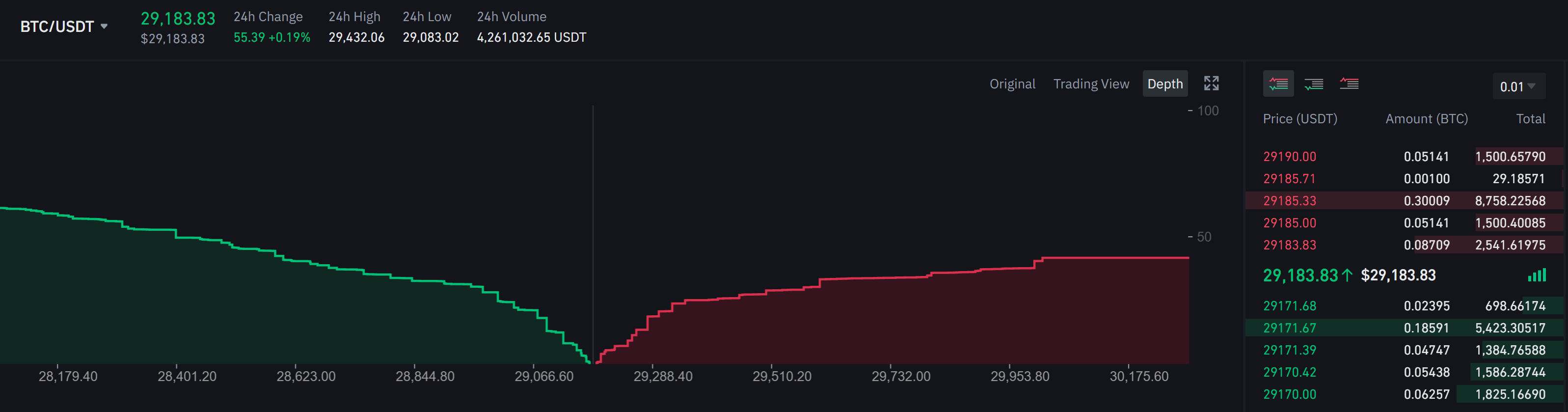
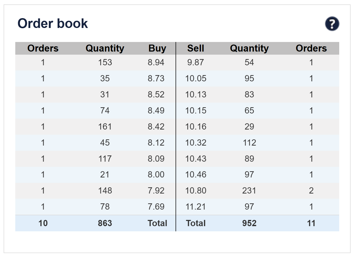
The “Buy” and “Sell” parts of the order book can be presented side by side (Table 1) or above each other (Tables 2 and 3) with the “Sell” part (in red) above the “Buy” part (in green) as the price limits of the sell limit orders are always higher than the price limits of the buy limit orders.
Table 1. Example of an order book (buy and sell parts presented side by side).
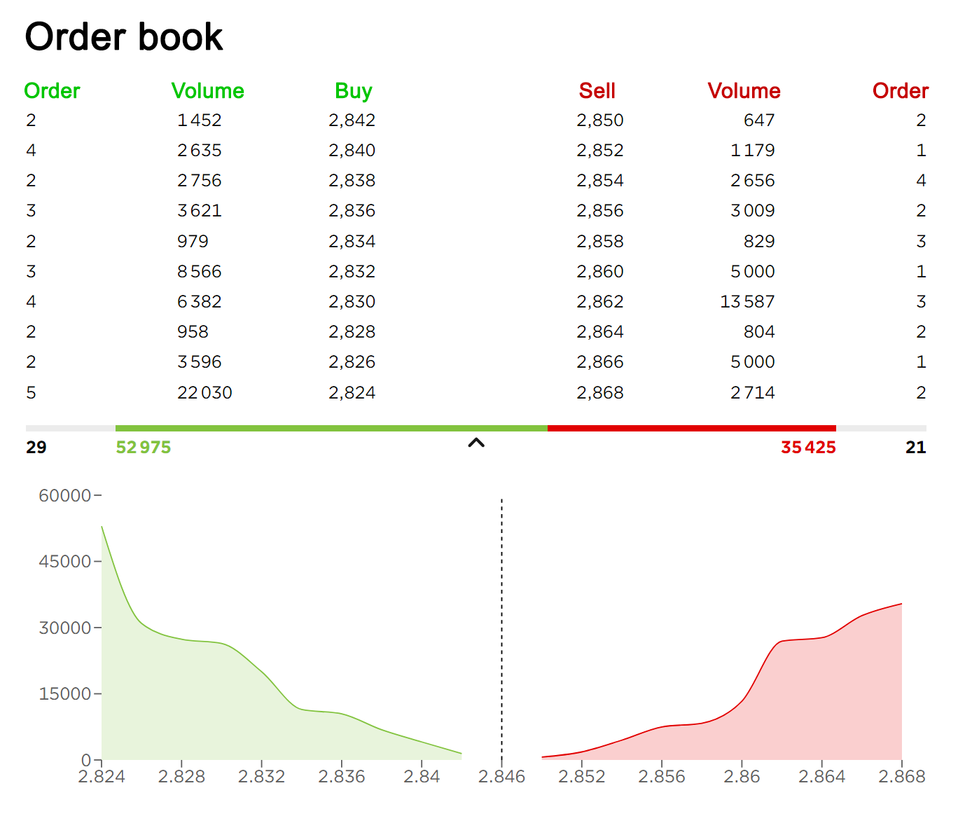
Source: online broker (Fortuneo).
Table 2. Example of an order book (buy and sell parts presented above each other).

Source: online broker (Cryptowatch).
Table 3. Example of an order book (buy and sell parts presented next to each other).
Source: online broker (Binance).
In a typical order book, the buy side is organized in descending order, meaning that the highest buy orders (i.e., the orders with the highest bid prices) are listed first, followed by the lower buy orders in descending order of price. The highest buy order in the book represents the best bid price, which is the highest price that any buyer is currently willing to pay for the asset.
On the other side of the order book, the sell side is organized in ascending order, with the lowest sell orders (i.e., the orders with the lowest ask prices) listed first, followed by the higher sell orders in ascending order of price. The lowest sell order in the book represents the best ask price, which is the lowest price that any seller is currently willing to accept for the asset.
This organization of the order book makes it easy for traders to see the current market depth and the best available bid and ask prices for an asset. When a buy order is executed at the best ask price or a sell order is executed at the best bid price, the order book is updated in real-time to reflect the new market depth and the new best bid and ask prices.
Table 4 below represents how the order book (limit order book) in trading simulations the SimTrade application.
Table 4. Order book in the SimTrade application.
You can understand how the order book works by launching a trading simulation on the SimTrade application.
The role of the order book in trading
As mentioned before, the order book is incredibly significant in trading. It acts as a market barometer, delivering real-time information about the supply and demand for an asset. Traders can also use the order book to determine market sentiment. If the bid side of the order book is strongly occupied, for example, it could imply that traders are optimistic on the asset. Thanks to the data in the order book, traders can get different information out of it.
Three characteristics of the order book
Market spread
The market spread, also known as the bid-ask spread, is the difference between the highest price a buyer is willing to pay for an asset (the bid price) and the lowest price a seller is willing to accept (the ask price) at a particular point in time.
The market spread is a reflection of the supply and demand for the asset in the market, and it represents the transaction cost of buying or selling the asset. In general, a narrow or tight spread indicates a liquid market with a high level of trading activity and a small transaction cost, while a wider spread suggests a less liquid market with lower trading activity and a higher transaction cost.
Market breadth
Market breadth is a measure of the overall health or direction of a market, sector, or index. It refers to the number of individual stocks that are participating in a market’s movement or trend, and can provide insight into the underlying strength or weakness of the market.
Market breadth is typically measured by comparing the number of advancing stocks (stocks that have increased in price) to the number of declining stocks (stocks that have decreased in price) over a given time period. This ratio is often expressed as a percentage or a ratio, with a higher percentage or ratio indicating a stronger market breadth and a lower percentage or ratio indicating weaker breadth.
For example, if there are 1,000 stocks in an index and 800 of them are increasing in price while 200 are decreasing, the market breadth ratio would be 4:1 or 80%. This would suggest that the market is broadly advancing, with a high number of stocks participating in the upward trend.
Market depth
Finally, market depth is a measure of the supply and demand of a security or financial instrument at different prices. It refers to the quantity of buy and sell orders that exist at different price levels in the market. Market depth is typically displayed in a market depth chart or order book.
It can provide valuable information to traders and investors about the current state of the market. A deep market with large quantities of buy and sell orders at various price levels can indicate a liquid market where trades can be executed quickly and with minimal impact on the market price. On the other hand, a shallow market with few orders at different price levels can indicate a less liquid market where trades may be more difficult to execute without significantly affecting the market price.
Analyzing order book data
Data from order books can be used to gain insight into market sentiment and trading opportunities. For example, traders can use the bid-ask spread to determine an asset’s liquidity. They can also examine the depth of the order book to determine the level of buying and selling interest in the asset. Traders can also use order book data to identify potential trading signals. For example, if the bid side of the order book is heavily populated at a certain price level, this could indicate that the asset’s price is likely to rise. On the other hand, if the ask side is heavily populated at a certain price level, it could indicate that the asset’s price is likely to fall.
Benefits of using order book data for trading
Using order book data can provide traders with a number of advantages.
For starters, it can be used to gauge market sentiment and identify potential trading opportunities.
Second, it can assist traders in more effectively managing risk. Traders can identify areas of support and resistance in order book data, which can then be used to set stop losses and take profits.
Finally, it can aid traders in the identification of potential trading signals. Traders can identify areas of potential buying and selling pressure in order book data, which can then be used to enter and exit trades.
How to use order book data for trading
Traders can use order book data to gain a competitive advantage in the markets. To accomplish this, they must first identify areas of support and resistance that can be used to set stop losses and profit targets.
Traders should also look for indications of buying and selling pressure in the order book. If the bid side of the order book is heavily populated at a certain price level, it could indicate that the asset’s price is likely to rise. On the other hand, if the ask side is heavily populated at a certain price level, it could indicate that the asset’s price is likely to fall.
Finally, traders should use trading software to automate their strategies. Trading bots can be set up to monitor order book data and execute trades based on it. This allows traders to capitalize on trading opportunities more quickly and efficiently.
Conclusion
To summarize, the order book is a vital instrument for financial market traders. It gives real-time information about an asset’s supply and demand, which can be used to gauge market mood and find potential trading opportunities. Traders can also utilize order book data to create stop losses and take profits and to automate their trading techniques. Traders might obtain an advantage in the markets by utilizing the power of the order book.
Related posts on the SimTrade blog
▶ Jayna MELWANI The impact of market orders on market liquidity
▶ Lokendra RATHORE Good-til-Cancelled (GTC) order and Immediate-or-Cancel (IOC) order
▶ Clara PINTO High-frequency trading and limit orders
▶ Akshit GUPTA Analysis of The Hummingbird Project movie
Useful resources
SimTrade course Trade orders
SimTrade course Market making
SimTrade simulations Market orders Limit orders
About the author
The article was written in March 2023 by Federico DE ROSSI (ESSEC Business School, Master in Strategy & Management of International Business (SMIB), 2020-2023).


 Source: computation by the author (data: Refinitiv Eikon).
 Source: computation by the author (Data: Refinitiv Eikon).
 Source: computation by the author (Data: Bloomberg)
 Source: computation by the author. (Data: Reuters Eikon)