Discovering the Secrets of a Bank Trading Room

Discovering the Secrets of a Bank Trading Room

David GONZALEZ

In this article, David GONZALEZ (ESSEC Business School, Global BBA, 2023-2024) delves into the amazing yet often concealed aspects that frequently transpire within different bank trading rooms. This investigation is rooted in his experiences at Banco Industrial y de Comercio Exterior (BICE).

BICE Bank

BICE Bank was founded in 1979 in Santiago, Chile, under the name Banco Industrial y de Comercio Exterior by a significant group of Chilean investors associated with some of the country’s leading export companies. Currently, BICE Bank has focused on providing services to high-income individuals in Chile. Currently, it is the seventh-highest commercial bank in Chile.

Logo of the company.
Logo of Banco BICE
Source: the company.

My Internship at BICE

Ever since I was young, I have been drawn to the financial markets. This was the primary reason that led me to select a nine-month internship in the Market Risk and Liquidity division, a component of the trading room at BICE Bank. My primary responsibility was to provide daily reports on various risk indicators to the trading room, with a particular emphasis on highlighting the changes resulting from different trades conducted during the day. In the following paragraphs, I will provide a brief overview of some of the main indicators I was tasked with explaining, after that, I am going to talk about some interesting things that every aspiring trader should know about this business.

The risk indicators that I was in charge of
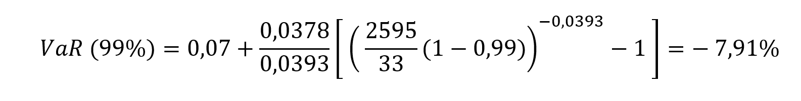
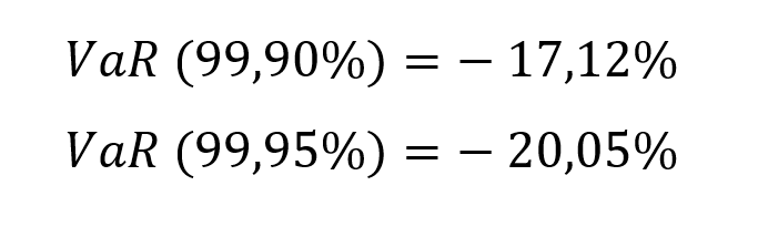
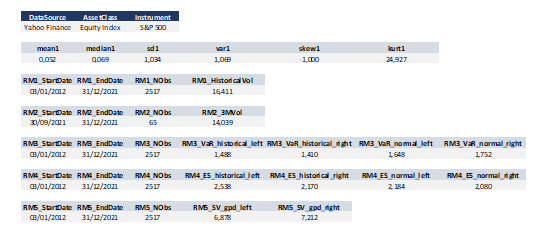
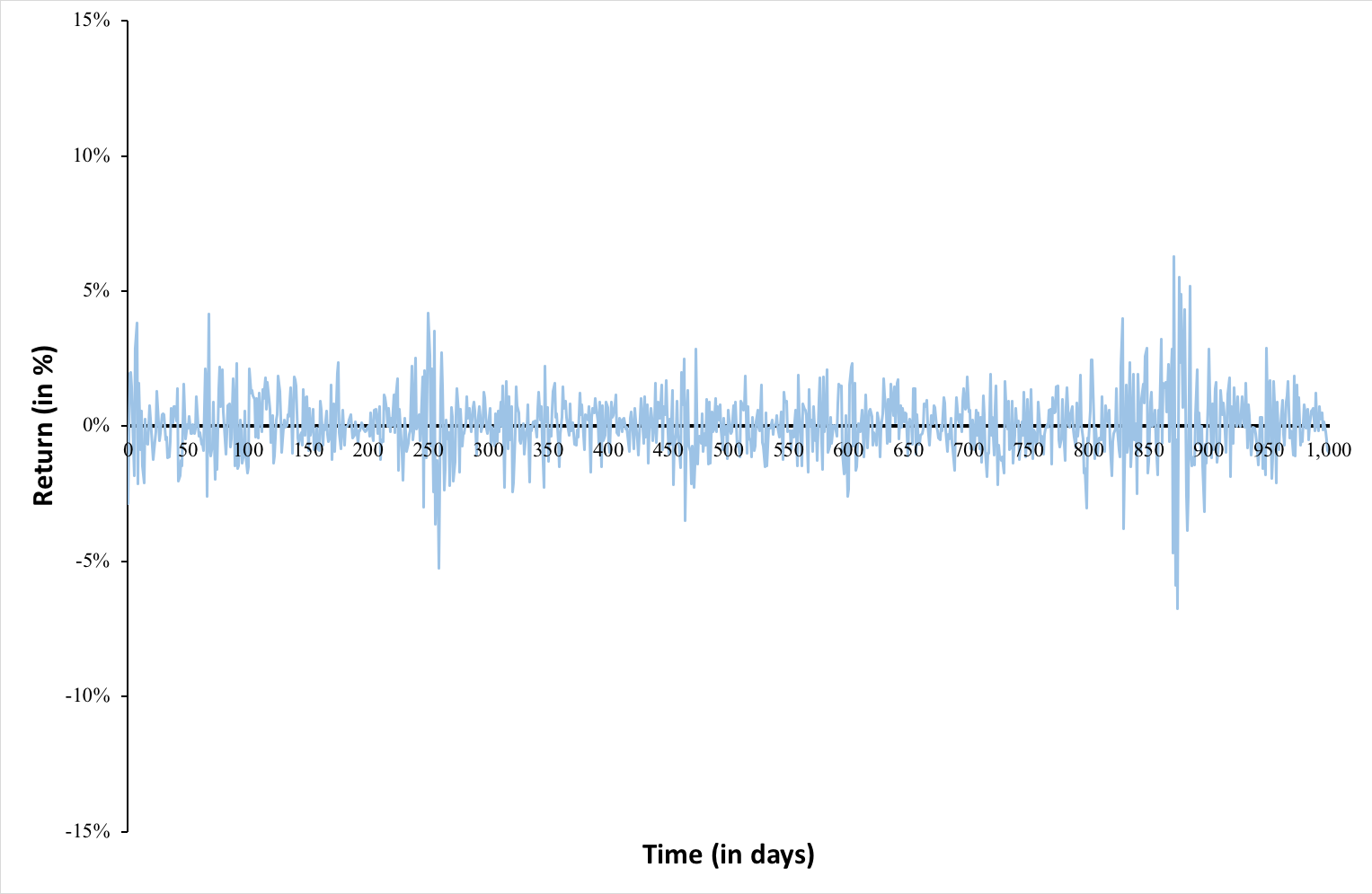
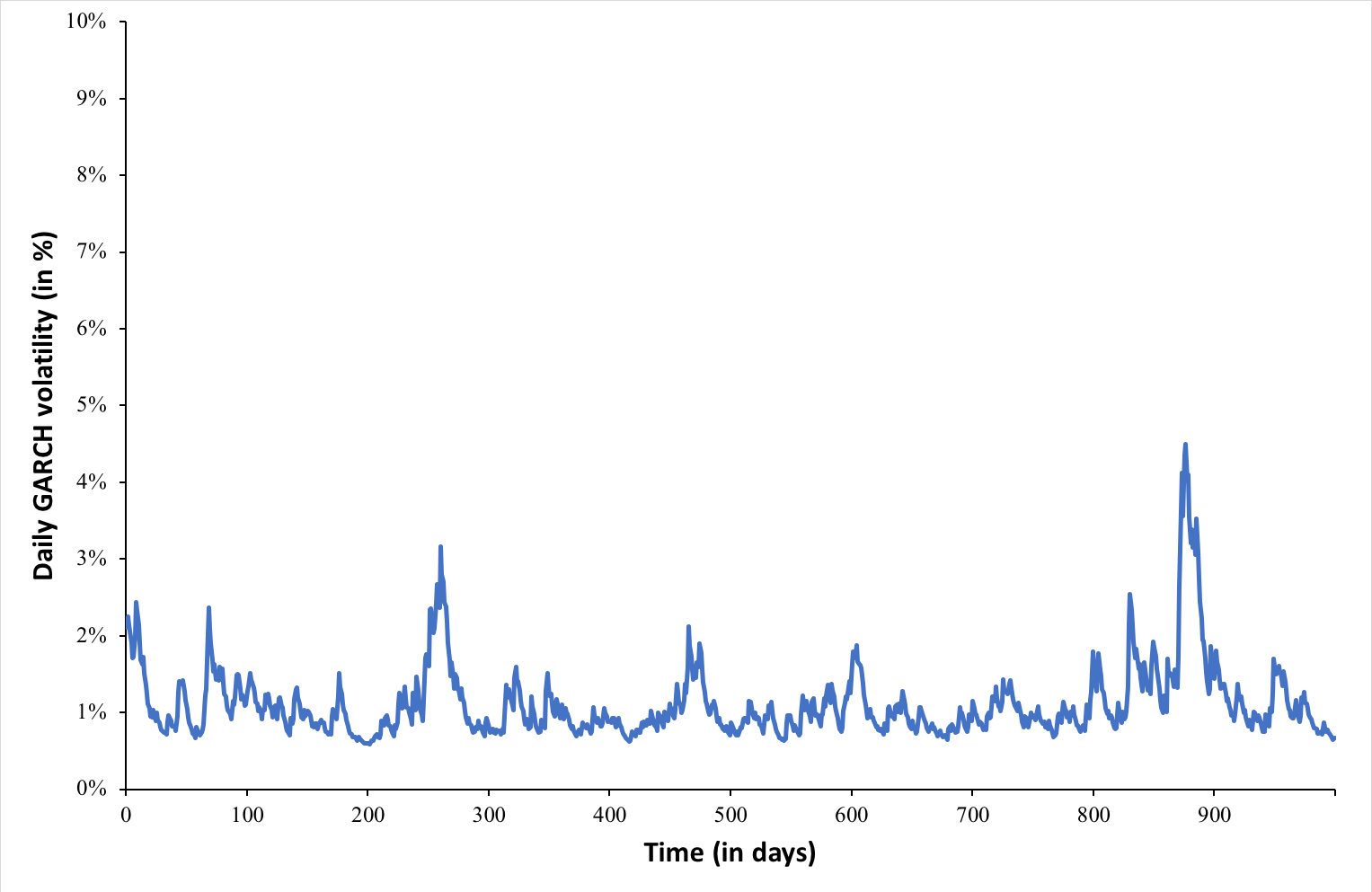
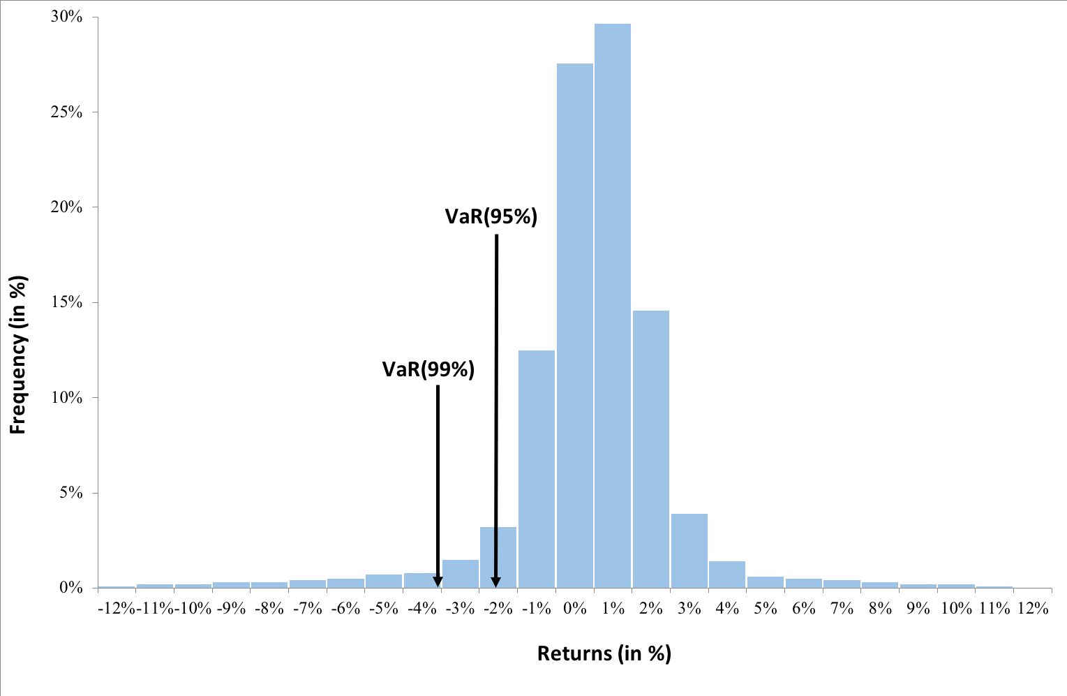
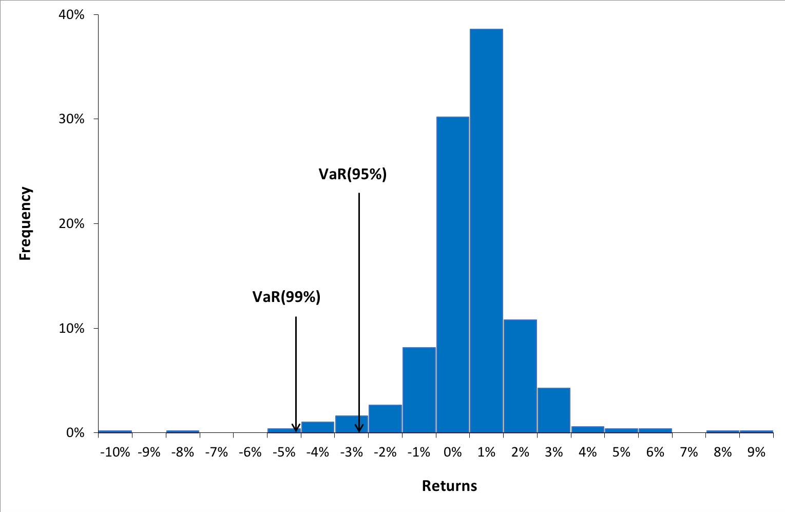
Value at Risk (VaR)

This indicator aims to quantify the worst-case scenario of losses in the bank’s portfolio, taking into account historical market data. In other words, it provides an estimate of the likely amount of money the portfolio could lose in a day of financial crisis (a stress scenario).

Present Value of 1 Basis Point (PV01)

This indicator seeks to quantify the potential loss in the portfolio resulting from a one-basis-point increase in interest rates. It is important to note that this indicator is applicable only to fixed-income assets, as it attempts to predict the change in the value of a bullet bond that is dependent on interest rate fluctuations.

Liquidity Coverage Ratio (LCR)

Have you ever heard of interbank loans? This indicator is of paramount importance to bankers as it assesses whether the bank possesses sufficient liquidity as required by regulatory standards or even for normal day-to-day operations. If the LCR falls below a certain threshold, the bank may need to enter into arrangements with a counterparty to borrow funds and restore this indicator to compliance.

Credit Value Adjustment (CVA)

Have you ever heard of the over-the-counter (OTC) market? Unlike centralized exchanges that guarantee the money or assets being traded, the OTC market lacks such centralized assurance. Banks frequently engage in OTC transactions, and the primary means by which they protect themselves against counterparty risk is through CVA. This is computed based on the credit rating of the counterparty. The CVA indicator reveals the bank’s exposure in relation to the counterparties with whom it conducts transactions.

Required skills and knowledge

In general, large trading rooms not only trade on the stock exchange, which is widely known, but they also engage in transactions in the over-the-counter (OTC) market. It was crucial for me to understand how this market operates, including what a swap is, what a forward contract entails, and how interest rates and inflation expectations influence the financial market. This knowledge was essential because I needed to stay informed about how macroeconomic factors or new transactions affected the bank’s portfolio. Every move in each risk indicator had to make economic or financial sense before being reported to the traders.

As for soft skills, effective communication when required was clearly important. Maintaining composure and seeking solutions rather than assigning blame when issues arose at work were vital skills as well. Furthermore, the ability to proactively seek solutions independently before seeking assistance from someone who might be occupied with their own tasks was crucial.

What just few people know (knowing the business)

Understanding Different Types of Trading Rooms: A Crucial Insight for Aspiring Traders

When I started working at BICE Bank, my boss told me that the bank had two trading rooms: one of them was the main trading room of the bank, and the other was the trading room of the stockbrokerage (which is a subsidiary of the bank). Obviously, this didn’t make sense to me, and I wondered, what is the reason for having two different trading rooms on two different floors of the building? When I expressed this concern to my boss, he explained, “It’s because they are oriented towards different sides. The main trading room focuses on the buy side, which means that traders manage, invest, and build portfolios while seeking returns within the risk level stipulated by the risk department. Usually, hedge funds, banks, insurance companies, and pension funds have this emphasis.” He continued, “The other trading room is part of the stockbrokerage, which is a subsidiary of this bank. They focus on the sell side. In this case, traders are responsible for executing transactions for clients who use our brokerage service. In other words, these traders don’t make decisions; they simply follow clients’ orders. Examples of this side include investment banks, brokerage firms, and market makers.”

Future traders must be clear on which side of the market they want to be on, so they can choose the right path for their careers. If the goal is to build their own portfolio and invest based on their own analyses and expectations, while assuming a higher level of risk, the trader should opt for the buy side. Conversely, if the aim is to avoid the risk of losses associated with maintaining a personal portfolio and only focus on achieving the best prices in the market, the sell side is the preferable choice. In this scenario, all the risk would be borne by the clients, as the trader would merely act as an intermediary between them and the market.

Financial concepts related my internship

The trader who triumphed over the 2008 crisis (Risks)

During my tenure at the bank, I had the privilege of meeting several senior traders, most of whom had over 20 years of experience in the market. One of them shared a fascinating story about how he navigated through the 2008 crisis.

Banks typically maintain a rather conservative investment policy, meaning they are risk averse. Consequently, one of the most common strategies is securities arbitrage (buying securities in a market where they are undervalued and selling them in other more expensive market). This strategy carries zero exposure, and profits are guaranteed when operating with substantial sums of money. This particular trader happened to be engaged in arbitrage on the day the 2008 financial crisis erupted. Upon realizing the unfolding catastrophe, he promptly closed his long positions remaining the shorts, that resulting in astronomical profits at a time when the global economy was collapsing.

Future traders looking to be on the buy side need to consider which financial institution is the best for advancing their career. Hedge funds, commercial banks, insurance companies, and pension fund managers tend to differ in terms of risk tolerance, either due to their own institutional policies or regulatory guidelines. For instance, in Chile, the regulatory commission does not allow commercial banks to invest in stocks.

Why a Chilean bank is concerned about federal reserve FED (Interest rates)

I had the fortune of gaining my experience at this bank during a period when the Fed and most central banks worldwide were raising their interest rates as a measure to control inflation stemming from the expansive policies implemented during the COVID-19 pandemic. I noticed that the traders were always closely monitoring the Fed’s announcements and whether they aligned with market expectations.

Intrigued by the heightened anticipation surrounding the market, I decided to seek insight from one of the traders. He offered the following explanation: “There are several factors contributing to this heightened attention. Primarily, monetary policy decisions in an inflationary environment tend to shape our trading strategies. On one hand, rate hikes affect all fixed-income assets, potentially causing our portfolio to depreciate in value and elevating risk indicators like VaR. Additionally, when the Federal Reserve tends to raise interest rates, it becomes more profitable for institutional investors to purchase bonds due to the relatively low levels of risk premium and liquidity premium demanded. Lastly, we also consider short positions in emerging market currencies since the dollar typically appreciates in the midst of Fed rate hikes.”

Federal Reserve announcements typically tend to influence financial markets. This is mainly because they shed light on the current state of the economy, enabling institutional investors to assess whether it is more profitable to invest in fixed income or equities. This assessment considers the risk premium and liquidity premium demanded from assets.

Liquidity the most important but the most avoided for banks (Banks Liquidity)

Every Monday afternoon, we held our weekly meeting where the latest developments were reported to the company’s top executives, including the CEO. During one such meeting, the bank’s CEO noticed that the bank’s liquidity indicators were quite comfortable, indicating an ample reserve of funds in the bank’s coffers.

Normally, customer deposits do not remain dormant in their accounts; instead, this money is put to use for investments or lent to other customers. Hence, the surplus liquidity captured the CEO’s attention. In the end, money entails a trade-off, and maintaining it in reserve can prove rather costly. The CEO raised a query regarding this with the head of the trading room, who clarified that the excess liquidity was a result of the impending release of the decision on whether to change the Chilean constitution or not, anticipated for that week. In anticipation of an adverse outcome, the trading room needed to uphold substantial liquidity to accommodate depositors wishing to withdraw their funds. The head of the trading room confirmed that, indeed, maintaining such high liquidity levels cost millions each day since interest rates were exceedingly high and the funds could have been invested. Nevertheless, this course of action was deemed necessary in light of the country’s political crisis.

Why should I be interested in this post?

Are you interested in pursuing a career in a trading room? Do you aspire to become a trader one day? If the answer is yes, you must read this post. By doing so, you will gain insights into how trading rooms operate and the various types of trading rooms available in the marketplace. Additionally, you will learn about some important concepts in finance, accompanied by an interesting story to introduce them.

Related posts on the SimTrade blog

Professional experiences

   ▶ All posts about Professional experiences

   ▶ Tanguy TONEL All posts about Professional experiences

   ▶ Shengyu ZHENG My experience as Actuarial Apprentice at La Mutuelle Générale

   ▶ Akshit GUPTA My apprenticeship experience within client services at BNP Paribas

Financial products

   ▶ Federico DE ROSSI Understanding the Order Book: How It Impacts Trading

   ▶ Alexandre VERLET Understanding financial derivatives: options

   ▶ Alexandre VERLET Understanding financial derivatives: futures

   ▶ Alexandre VERLET Understanding financial derivatives: swaps

   ▶ Alexandre VERLET Understanding financial derivatives: forwards

Useful resources

Hull J.C. (2021) Options, Futures, and Other Derivatives Pearson, 11th Edition.

Banco BICE (2022) Memoria Anual.

About the author

The article was written in December 2023 by David Gonzalez (ESSEC Business School, Grande Ecole Program – Global BBA, 2023-2024).

Application de la théorie des valeurs extrêmes en finance de marchés

Gabriel FILJA

Dans cet article, Gabriel FILJA (ESSEC Business School, Executive Master in Senior Bank Management, 2022-2023 & Head of Hedging à Convera) présente des applications de la théorie des valeurs extrêmes en finance de marchés et notamment en gestion des risques de marchés.

Principe

La théorie des valeurs extrêmes (TVE), appelé théorème de Fisher-Tippet-Gnedenko tente de fournir une caractérisation complète du comportement de la queue pour tous les types de distributions de probabilités.

La théorie des valeurs extrêmes montre que la loi asymptotique des rentabilités minimale et maximale a une forme bien déterminée qui est largement indépendante du processus de rentabilités lui-même (le lien entre les deux distributions apparaît en particulier dans la valeur de l’indice de queue qui reflète le poids des queues de distribution). L’intérêt de la TVE dans la gestion du risque c’est de pouvoir calculer le quantile au-delà de 99% du seuil de confiance dans le cadre des stress tests ou de la publication des exigences réglementaires.

Gnedenko a démontré en 1943 par la Théorie des valeurs extrêmes la propriété qui s’applique à des nombreuses distributions de probabilités. Soit F(x) la fonction de répartition d’une variable x. u est une valeur de x située dans la partie droite de la queue de distribution.

La probabilité que x soit compris entre u et u+y est de F(y+u) – F(u) et la probabilité que x soit supérieur à u est 1-F(u). Soit Fu(y) la probabilité conditionnelle que x soit compris entre u et u+y sachant que x>u∶

Probabilité conditionnelle

Estimation des paramètres

Selon les résultats de Gnedenko, pour un grand nombre de distribution, cela converge vers une distribution généralisée de Pareto au fur et à mesure que u augmente :

Distribution_généralisée_Pareto

β est le paramètre d’échelle représente la dispersion de la loi des extrêmes
ξ est l’indice de queue qui mesure l’épaisseur de la queue et la forme

Selon la valeur de l’indice de queue, on distingue trois formes dedistribiution d’extrêmes :

  • Frechet ξ > 0
  • Weibull ξ < 0
  • Gumbel ξ = 0

L’indice de queue ξ reflète le poids des extrêmes dans la distribution des rentabilités. Une valeur positive de l’indice de queue signifie que les extrêmes n’ont pas de rôle important puisque la variable est bornée. Une valeur nulle donne relativement peu d’extrêmes alors qu’une valeur négative implique un grand nombre d’extrêmes (c’est le cas de la loi normale).

Figure 1 : Densité des lois des valeurs extrêmes
 Densité des lois des valeurs extrêmes
Source : auteur.

Tableau 1 : Fonctions de distribution des valeurs extrêmes pour un ξ > 0, loi de Frechet, ξ < 0 loi de Weibull et ξ = 0, loi de Gumbel. Fonctions de distribution des valeurs extrêmes
Source : auteur.

Les paramètres β et ξ sont estimés par la méthode de maximum de vraisemblance. D’abord il faut définir u (valeur proche du 95e centile par exemple). Une des méthodes pour déterminer ce seuil, c’est la technique appelée Peak Over Threshold (POT), ou méthode des excès au-delà d’un seuil qui se focalise sur les observations qui dépassent un certain seuil donné. Au lieu de considérer les valeurs maximales ou les plus grandes valeurs, cette méthode consiste à examiner toutes les observations qui franchissent un seuil élevé préalablement fixé.
L’objectif est de sélectionner un seuil adéquat et d’analyser les excès qui en découlent. Ensuite nous trions les résultats par ordre décroissant pour obtenir les observations telles que x>u et leur nombre total.

Nous étudions maintenant les rentabilités extrêmes pour l’action Société Générale sur la période 2011-2021. La Figure 2 représentes rentabilités journalières de l’action et les rentabilités extrêmes négatives obtenues avec l’approche des dépassements de seuil (Peak Over Threshold ou POT). Avec le seuil retenu de -7%, on obtient 33 dépassements sur 2 595 rentabilités journalières de la période 2011 à 2021.

Figure 2 : Sélection des rentabilités extrêmes négatives pour l’action Société Générale selon l’approche Peak Over Threshold (POT)
Sélection des rentabilités extrêmes pour le titre Société Genérale
Source : auteur.

Méthode d’estimation statistique

Nous allons maintenant voir comment déterminer les β et ξ en utilisant la fonction de maximum de vraisemblance qui s’écrit :

Fonction de vraisemblance

Pour un échantillon de n observations, l’estimation de 1-F(u) est nu/n. Dans ce cas, la probabilité inconditionnelle de x>u+y vaut :

Fonction de vraisemblance

Et l’estimateur de la queue de distribution de probabilité cumulée de x (pour un grand) est :

Estimateur queue distribution

Mon travail personnel a consisté à estimer le paramètre d’échelle β et le paramètre de queue ξ à partir de la formule par le maximum de vraisemblance en utilisant le solveur Excel. Nous avons précédemment déterminé n=0,07 par la méthode de POT en Figure 2, et n_u= 2595

Ainsi nous obtenons β=0,0378 et ξ=0,0393 ce qui maximise par la méthode du maximum de vraisemblance la somme du logarithme des valeurs extrêmes à un total de 73,77.

Estimation de la VaR TVE

Pour calculer le VaR au seuil q, nous obtenons F(VaR) = q

VaR TVE

Mon travail personnel a consisté à estimer la VaR du titre de la Société Générale de la période de 2011 à 2021 sur un total de 2595 cotations avec 33 dépassements de seuil (-7%). En appliquant les données obtenues à la formule nous obtenons :

VaR 99% Société Générale

Puis nous estimons la VaR à 99,90% et 99,95% :

VaR 99,90% Société Générale

Il n’est pas surprenant que l’extrapolation à la queue d’une distribution de probabilité soit difficile, pas parce qu’il est difficile d’identifier des distributions de probabilité possibles qui pourraient correspondre aux données observées (il est relativement facile de trouver de nombreuses distributions possibles différentes), mais parce que l’éventail des réponses qui peuvent vraisemblablement être obtenues peut être très large, en particulier si nous voulons extrapoler dans la queue lointaine où il peut y avoir peu ou pas de points d’observation directement applicables.

La théorie des valeurs extrêmes, si elle est utilisée pour modéliser le comportement de la queue au-delà de la portée de l’ensemble de données observées, est une forme d’extrapolation. Une partie de la cause du comportement à queue épaisse (fat tail) est l’impact que le comportement humain (y compris le sentiment des investisseurs) a sur le comportement du marché.

En quoi ça peut m’intéresser ?

Nous pouvons ainsi mener des stress tests en utilisant la théorie des valeurs extrêmes et évaluer les impacts sur le bilan de la banque ou encore déterminer les limites de risques pour le trading et obtenir ainsi une meilleure estimation du worst case scenario.

Autres articles sur le blog SimTrade

▶ Shengyu ZHENG Catégories de mesures de risques

▶ Shengyu ZHENG Moments de la distribution

▶ Shengyu ZHENG Extreme Value Theory: the Block-Maxima approach and the Peak-Over-Threshold approach

Ressources

Articles académiques

Falk M., J. Hüsler, et R.-D. Reiss, Laws of Small Numbers: Extremes and Rare Events. Basel: Springer Basel, 2011. doi: 10.1007/978-3-0348-0009-9.

Gilli M. et E. Këllezi, « An Application of Extreme Value Theory for Measuring Financial Risk », Comput Econ, vol. 27, no 2, p. 207‑228, mai 2006, doi: 10.1007/s10614-006-9025-7.

Gkillas K. and F. Longin (2018) Financial market activity under capital controls: lessons from extreme events Economics Letters, 171, 10-13.

Gnedenko B., « Sur La Distribution Limite Du Terme Maximum D’Une Serie Aleatoire », Annals of Mathematics, vol. 44, no 3, p. 423‑453, 1943, doi: 10.2307/1968974.

Hull J.et A. White, « Optimal delta hedging for options », Journal of Banking & Finance, vol. 82, p. 180‑190, sept. 2017, doi: 10.1016/j.jbankfin.2017.05.006.

Longin F. (1996) The asymptotic distribution of extreme stock market returns Journal of Business, 63, 383-408.

Longin F. (2000) From VaR to stress testing : the extreme value approach Journal of Banking and Finance, 24, 1097-1130.

Longin F. (2016) Extreme events in finance: a handbook of extreme value theory and its applications Wiley Editions.

Longin F. and B. Solnik (2001) Extreme Correlation of International Equity Markets, The Journal of Finance, 56, 649-676.

Roncalli T. et G. Riboulet, « Stress testing et théorie des valeurs extrêmes : une vision quantitée du risque extrême ».

Sites internet

Extreme Events in Finance

A propos de l’auteur

Cet article a été écrit en juillet 2023 par Gabriel FILJA (ESSEC Business School, Executive Master in Senior Bank Management, 2022-2023 & Head of Hedging à Convera).

Mesures de risques

Mesures de risques

Shengyu ZHENG

Dans cet article, Shengyu ZHENG (ESSEC Business School, Grande Ecole Program – Master in Management, 2020-2023) présente les mesures de risques basées sur la distribution statistique des rentabilités d’une position de marché, ce qui est une approche possible pour mesurer les risques (comme expliqué dans mon article Catégorie de mesures de risques).

Les mesures de risques basées sur la distribution statistique sont des outils largement utilisés pour la gestion des risques par de nombreux de participants du marché, dont les traders, les teneurs de marché, les gestionnaires d’actifs, les assureurs, les institutions réglementaires et les investisseurs.

Ecart-type / Variance

La variance (moment d’ordre deux de la distribution statistique) est une mesure de la dispersion des valeurs par rapport à la moyenne. La variance est définie par

Var(X) = σ 2 = 𝔼[(X-μ)2]

Par construction, la variance est toujours positive (ou nulle pour une variable aléatoire constante).

En finance, l’écart-type (racine carrée de la variance) mesure la volatilité des actifs financiers. Un écart-type (ou une variance élevée) indique une dispersion plus importante, et donc un risque plus important, ce n’est pas apprécié par les investisseurs qui ont de l’aversion au risque. L’écart-type (ou la variance) est un paramètre clef dans la théorie moderne du portefeuille de Markowitz.

La variance a un estimateur non biaisé donné par

Ŝ2 = (∑ni=1(xi – X̄)2)/(n-1)

Value at Risque (VaR)

La Value at Risque (VaR, parfois traduite comme valeur en enjeu) est une notion classique pour mesurer les risques de perte d’un actif. Elle correspond au montant de perte d’une position qui ne devrait être dépassé qu’avec une probabilité donnée sur un horizon précisé, ou autrement dit, au montant de la pire perte attendue sur un horizon de temps pour un certain niveau de confiance. Elle est essentiellement le quantile de la probabilité donnée de la distribution de perte (rendement négatif).

Dans le langage mathématique, la VaR est définie comme :

VaRα = inf{y ∈ : ℙ[L>y] ≤ 1 – α} = inf{ y ∈ : ℙ[L ≤ y] ≥ α }

VaRα = qα(F) ≔ F(α)

α est la probabilité donnée ; L est une variable aléatoire de montant de perte ; F est la distribution cumulative de perte (rendement négatif), ce qui est continue et strictement croissante ; F est l’inverse de F.

Les organismes financiers se servent assez souvent de cette mesure pour la rapidité et la simplicité des calculs. Toutefois, elle présente certaines lacunes. Elle n’est pas une mesure cohérente. Cela dit, l’addition des VaRs de 2 portefeuilles aurait aucun sens. À part cela, basée sur une hypothèse gaussienne, elle ne tient pas compte de la gravité et la possibilité des évènements extrêmes, tant que les distributions du marché financier sont, pour la plupart, leptokurtiques.

Expected Shortfall (ES)

L’Expected shortfall (ES) est la perte espérée pendant N jours conditionnellement au fait de se situer dans la queue (1 – α) de la distribution des gains ou des pertes (N est l’horizon temporel et α est le niveau de confiance). Autrement dit, elle est la moyenne des pertes lors d’un choc qui est pire que α% cas. L’ES est donc toujours supérieure à la VaR. Elle est souvent appelée VaR conditionnelle (CVaR).

ESα = ∫ 1α (VaRβ(L) dβ)/(1 – α)

En comparaison de la VaR, ES est capable de montrer la gravité de perte dans des cas extrêmes. Ce point est primordial pour la gestion moderne de risques qui souligne la résilience surtout en cas d’extrême.

La VaR a été préférée par les participants du marché financier depuis longtemps, mais les défauts importants présentés ci-dessus ont occasionné des reproches, notamment face aux souvenances des crises majeures. L’ES, rendant compte des évènements extrêmes, tend désormais à s’imposer.

Stress Value (SV)

La Stress Value (SV) est un concept similaire à la VaR. Comme la VaR, la SV est définie comme un quantile. Pour la SV, la probabilité associée au quantile est proche de 1 (par exemple, un quantile de 99.5% pour la SV, en comparaison d’un quantile de 95% pour la VaR habituelle). La SV décrit plus précisément les pertes extrêmes.

L’estimation paramétrique de SV normalement s’appuie sur la théorie de valeurs extrêmes (EVT), alors que celle de VaR est basée sur une distribution gaussienne.

Programme R pour calculer les mesures de risques

Vous pouvez télécharger ci-dessous un programme R qui permet de calculer les mesures de risques d’une position de marché (construite à partir d’indices d’actions ou d’autres actifs).

Mesures_de_risque

Voici est une liste des symboles d’actif (“tickers”) que nous pouvons intégrer dans le programme R.
Download the ticker list to calculate risk measures

Example de calcul des mesures de risque de l’indice S&P 500

Ce programme nous permet de calculer rapidement des mesures de risque pour des actifs financiers dont les données historiques peuvent être téléchargées sur le site Yahoo! Finance. Je vous présente une analyse de risque pour l’indice S&P 500.

En saisissant la date de début comme 01/01/2012 et la date d’arrêté comme 01/01/2022, ce programme est en mesure de calculer les mesures de risque pour toute la période considérée.

Vous trouverez ci-dessous les mesures de risque calculées pour toute la période : la volatilité historique, la volatilité conditionnelle sur les 3 derniers mois, VaR, ES et SV.

risk mesures S&P 500

Autres articles sur le blog SimTrade

   ▶ Shengyu ZHENG Catégories de mesures de risques

   ▶ Shengyu ZHENG Moments de la distribution

   ▶ Shengyu ZHENG Extreme Value Theory: the Block-Maxima approach and the Peak-Over-Threshold approach

   ▶ Youssef LOURAOUI Markowitz Modern Portfolio Theory

Ressources

Articles académiques

Merton R.C. (1980) On estimating the expected return on the market: An exploratory investigation, Journal of Financial Economics, 8:4, 323-361.

Hull J. (2010) Gestion des risques et institutions financières, Pearson, Glossaire français-anglais.

Données

Yahoo! Finance

A propos de l’auteur

Cet article a été écrit en février 2023 par Shengyu ZHENG (ESSEC Business School, Grande Ecole Program – Master in Management, 2020-2023).

The Monte Carlo simulation method for VaR calculation

Jayati WALIA

In this article, Jayati WALIA (ESSEC Business School, Grande Ecole – Master in Management, 2019-2022) explains the Monte Carlo simulation method for VaR calculation.

Introduction

Monte Carlo simulations are a broad class of computational algorithms that rely majorly on repeated random sampling to obtain numerical results. The underlying concept is to model the multiple possible outcomes of an uncertain event. It is a technique used to understand the impact of risk and uncertainty in prediction and forecasting models.

The Monte Carlo simulation method was invented by John von Neumann (Hungarian-American mathematician and computer scientist) and Stanislaw Ulam (Polish mathematician) during World War II to improve decision making under uncertain conditions. It is named after the popular gambling destination Monte Carlo, located in Monaco and home to many famous casinos. This is because the random outcomes in the Monte Carlo modeling technique can be compared to games like roulette, dice and slot machines. In his autobiography, ‘Adventures of a Mathematician’, Ulam mentions that the method was named in honor of his uncle, who was a gambler.

Calculating VaR using Monte Carlo simulations

The basic concept behind the Monte Carlo approach is to repeatedly run a large number of simulations of a random process for a variable of interest (such as asset returns in finance) covering a wide range of possible scenarios. These variables are drawn from pre-specified probability distributions that are assumed to be known, including the analytical function and its parameters. Thus, Monte Carlo simulations inherently try to recreate the distribution of the return of a position, from which VaR can be computed.

Consider the CAC40 index as our asset of interest for which we will compute the VaR using Monte Carlo simulations.

The first step in the simulation is choosing a stochastic model for the behavior of our random variable (the return on the CAC 40 index in our case).
A common model is the normal distribution; however, in this case, we can easily compute the VaR from the normal distribution itself. The Monte Carlo simulation approach is more relevant when the stochastic model is more complex or when the asset is more complex, leading to difficulties to compute the VaR. For example, if we assume that returns follow a GARCH process, the (unconditional) VaR has to be computed with the Monte Carlo simulation methods. Similarly, if we consider complex financial products like options, the VaR has to be computed with the Monte Carlo simulation methods.

In this post, we compare the Monte Carlo simulation method with the historical method and the variance-covariance method. Thus, we simulate returns for the CAC40 index using the GARCH (1,1) model.
Figure 1 and 2 illustrate the GARCH simulated daily returns and volatility for the CAC40 index.

Figure 1. Simulated GARCH daily returns for the CAC40 index.
img_SimTrade_CAC40_GARCH_ret
Source: computation by the author.

Figure 2. Simulated GARCH daily volatility for the CAC40 index.
img_SimTrade_CAC40_GARCH_vol
Source: computation by the author.

Next, we sort the distribution of simulated returns in ascending order (basically in order of worst to best returns observed over the period). We can now interpret the VaR for the CAC40 index in one-day time horizon based on a selected confidence level (probability).

For instance, if we select a confidence level of 99%, then our VaR estimate corresponds to the 1st percentile of the probability distribution of daily returns (the bottom 1% of returns). In other words, there are 99% chances that we will not obtain a loss greater than our VaR estimate (for the 99% confidence level). Similarly, VaR for a 95% confidence level corresponds to bottom 5% of the returns.

Figure 3 below represents the unconditional probability distribution of returns for the CAC40 index assuming a GARCH process for the returns.

Figure 3. Probability distribution of returns for the CAC40 index.
img_SimTrade_CAC40_MonteCarloVaR
Source: computation by the author.

From the above graph, we can interpret VaR for 99% confidence level as -3% i.e., there is a 99% probability that daily returns we obtain in future are greater than -3%. Similarly, VaR for 95% confidence level as -1.72% i.e., there is a 95% probability that daily returns we obtain in future are greater than -1.72%.

You can download below the Excel file for computation of VaR for CAC40 stock using Monte Carlo method involving GARCH(1,1) model for simulation of returns.

Download the Excel file to compute the Monte Carlo VaR

Advantages and limitations of Monte Carlo method for VaR

The Monte Carlo method is a very powerful approach to VAR due its flexibility. It can potentially account for a wide range of scenarios. The simulations also account for nonlinear exposures and complex pricing patterns. In principle, the simulations can be extended to longer time horizons, which is essential for risk measurement and to model more complex models of expected returns.

This approach, however, involves investments in intellectual and systems development. It also requires more computing power than simpler methods since the more is the number of simulations generated, the wider is the range of potential scenarios or outcomes modelled and hence, greater would be the potential accuracy of VaR estimate. In practical applications, VaR measures using Monte Carlo simulation often takes hours to run. Time requirements, however, are being reduced significantly by advances in computer software and faster valuation methods.

Related posts on the SimTrade blog

   ▶ Jayati WALIA Quantitative Risk Management

   ▶ Jayati WALIA Value at Risk

   ▶ Jayati WALIA The historical method for VaR calculation

   ▶ Jayati WALIA The variance-covariance method for VaR calculation

   ▶ Jayati WALIA Brownian Motion in Finance

Useful resources

Jorion P. (2007) Value at Risk, Third Edition, Chapter 12 – Monte Carlo Methods, 321-326.

About the author

The article was written in March 2022 by Jayati WALIA (ESSEC Business School, Grande Ecole Program – Master in Management, 2019-2022).

The historical method for VaR calculation

Jayati WALIA

In this article, Jayati WALIA (ESSEC Business School, Grande Ecole Program – Master in Management, 2019-2022) presents the historical method for VaR calculation.

Introduction

A key factor that forms the backbone for risk management is the measure of those potential losses that an institution is exposed to any investment. Various risk measures are used for this purpose and Value at Risk (VaR) is the most commonly used risk measure to quantify the level of risk and implement risk management.

VaR is typically defined as the maximum loss which should not be exceeded during a specific time period with a given probability level (or ‘confidence level’). VaR is used extensively to determine the level of risk exposure of an investment, portfolio or firm and calculate the extent of potential losses. Thus, VaR attempts to measure the risk of unexpected changes in prices (or return rates) within a given period. Mathematically, the VaR corresponds to the quantile of the distribution of returns.

The two key elements of VaR are a fixed period of time (say one or ten days) over which risk is assessed and a confidence level which is essentially the probability of the occurrence of loss-causing event (say 95% or 99%). There are various methods used to compute the VaR. In this post, we discuss in detail the historical method which is a popular way of estimating VaR.

Calculating VaR using the historical method

Historical VaR is a non-parametric method of VaR calculation. This methodology is based on the approach that the pattern of historical returns is indicative of the pattern of future returns.

The first step is to collect data on movements in market variables (such as equity prices, interest rates, commodity prices, etc.) over a long time period. Consider the daily price movements for CAC40 index within the past 2 years (512 trading days). We thus have 512 scenarios or cases that will act as our guide for future performance of the index i.e., the past 512 days will be representative of what will happen tomorrow.

For each day, we calculate the percentage change in price for the CAC40 index that defines our probability distribution for daily gains or losses. We can express the daily rate of returns for the index as:
img_historicalVaR_returns_formula

Where Rt represents the (arithmetic) return over the period [t-1, t] and Pt the price at time t (the closing price for daily data). Note that the logarithmic return is sometimes used (see my post on Returns).

Next, we sort the distribution of historical returns in ascending order (basically in order of worst to best returns observed over the period). We can now interpret the VaR for the CAC40 index in one-day time horizon based on a selected confidence level (probability).

Since the historical VaR is estimated directly from data without estimating or assuming any other parameters, hence it is a non-parametric method.

For instance, if we select a confidence level of 99%, then our VaR estimate corresponds to the 1st percentile of the probability distribution of daily returns (the top 1% of worst returns). In other words, there are 99% chances that we will not obtain a loss greater than our VaR estimate (for the 99% confidence level). Similarly, VaR for a 95% confidence level corresponds to top 5% of the worst returns.

Figure 1. Probability distribution of returns for the CAC40 index.
Historical method VaR
Source: computation by the author (data source: Bloomberg).

You can download below the Excel file for the VaR calculation with the historical method. The historical distribution is estimated with historical data from the CAC 40 index.

Download the Excel file to compute the historical VaR

From the above graph, we can interpret VaR for 90% confidence level as -3.99% i.e., there is a 90% probability that daily returns we obtain in future are greater than -3.99%. Similarly, VaR for 99% confidence level as -5.60% i.e., there is a 99% probability that daily returns we obtain in future are greater than -5.60%.

Advantages and limitations of the historical method

The historical method is a simple and fast method to calculate VaR. For a portfolio, it eliminates the need to estimate the variance-covariance matrix and simplifies the computations especially in cases of portfolios with a large number of assets. This method is also intuitive. VaR corresponds to a large loss sustained over an historical period that is known. Hence users can go back in time and explain the circumstances behind the VaR measure.

On the other hand, the historical method has a few of drawbacks. The assumption is that the past represents the immediate future is highly unlikely in the real world. Also, if the horizon window omits important events (like stock market booms and crashes), the distribution will not be well represented. Its calculation is only as strong as the number of correct data points measured that fully represent changing market dynamics even capturing crisis events that may have occurred such as the Covid-19 crisis in 2020 or the financial crisis in 2008. In fact, even if the data does capture all possible historical dynamics, it may not be sufficient because market will never entirely replicate past movements. Finally, the method assumes that the distribution is stationary. In practice, there may be significant and predictable time variation in risk.

Related posts on the SimTrade blog

   ▶ Jayati WALIA Quantitative Risk Management

   ▶ Jayati WALIA Value at Risk

   ▶ Jayati WALIA The variance-covariance method for VaR calculation

   ▶ Jayati WALIA The Monte Carlo simulation method for VaR calculation

Useful resources

Jorion, P. (2007) Value at Risk , Third Edition, Chapter 10 – VaR Methods, 276-279.

Longin F. (2000) From VaR to stress testing : the extreme value approach Journal of Banking and Finance, 24, 1097-1130.

About the author

The article was written in December 2021 by Jayati WALIA (ESSEC Business School, Grande Ecole Program – Master in Management, 2019-2022).