

In this article, Jayati WALIA (ESSEC Business School, Grande Ecole Program – Master in Management, 2019-2022) explains how returns of financial assets are computed and their interpretation in the world of finance.
Introduction
The main focus of any investment in financial markets is to make maximum profits within a coherent risk level. Returns in finance is a metric that inherently refers to the change in the value of any investment. Positive values of returns are interpreted as gains whereas negative values are interpreted as losses.
Returns are generally computed over standardized frequencies such as daily, monthly, yearly, etc. They can also be computed for specific time periods such as the holding period for ease of comparison and analysis.
Computation of returns
Consider an asset for a time period [t -1, t] with an initial price Pt-1 at time t-1 and final price Pt at time t (one period, two dates). Different forms of defining returns for the asset over period [t -1, t] are discussed below.
Arithmetic (percentage) returns
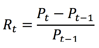
This is the simplest way for computation of returns.
The return over the period [t -1, t], denoted by Rt, is expressed as:
Logarithmic returns
Logarithmic returns (or log returns) are also used commonly to express investment returns. The log return over the period [t-1, t], denoted by Rt is expressed as:
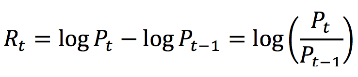
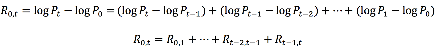
Log returns provide the property of time-additivity to the returns which essentially means that the log returns over a given period can be simply added together to compute the total return over subperiods. This feature is particularly useful in statistical analysis and reduction of algorithmic complexity.
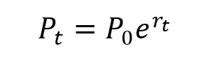
Log returns are also known as continuously compounded returns because the rate of log returns is equivalent to the continuously compounding interest rate for the asset at price P0 and time period t.
Link between arithmetic and logarithmic returns
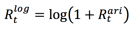
The arithmetic return (Rari) and the logarithmic return (Rlog) are linked by the following formula:
Components of total returns
The total return on an investment is essentially composed of two components: the yield and the capital gain (or loss). The yield refers to the periodic income or cash-flows that may be received on the investment. For example, for an investment in stocks, the yield corresponds to the revenues of dividends while for bonds, it corresponds to interest payments.
On the other hand, capital gain (or loss) refers to the appreciation (or depreciation) in the price of the investment. Thus, the capital gain (or loss) for any asset is essentially the price change in the asset.
Total returns for a stock over the period [t -1, t], denoted by Rt, can hence be expressed as:
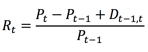
Where
Pt: Stock price at time t
Pt-1: Stock price at time t-1
Dt-1,t: Dividend obtained over the period [t -1, t]
Price changes and returns
Consider a stock with an initial price of 100€ at time t=0. Suppose the stock price drops to 50€ at time t=1. Thus, there is a change of -50% (minus sign representing the decrease in price) in the initial stock price.
Now for the stock price to reach back to its initial price (100€ in this case) at time t=2 from its price of 50€ at time t=1, it will require an increase of (100€-50€)/50€ = 100%. With arithmetic returns, the increase (+100%) has to be higher than the decrease (-50%).
Similarly, for a price drop of -25% in the initial stock price of 100€, we would require an increase of 33% in the next time period to reach back the initial stock price. Figure 1 illustrates this asymmetry between positive and negative arithmetic returns.
Figure 1. Evolution of price change as a measure of arithmetic returns.
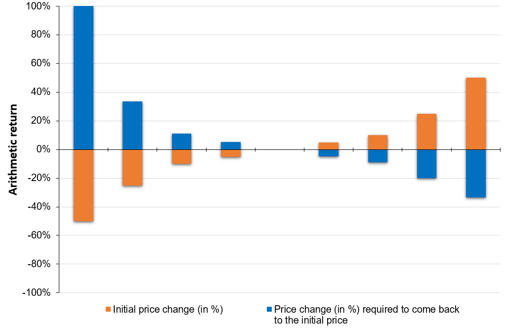
Source: computation by the author.
If the return is defined as a logarithmic return, there is a symmetry between positive and negative logarithmic returns as illustrated in Figure 2.
Figure 2. Evolution of price change as a measure of logarithmic returns.
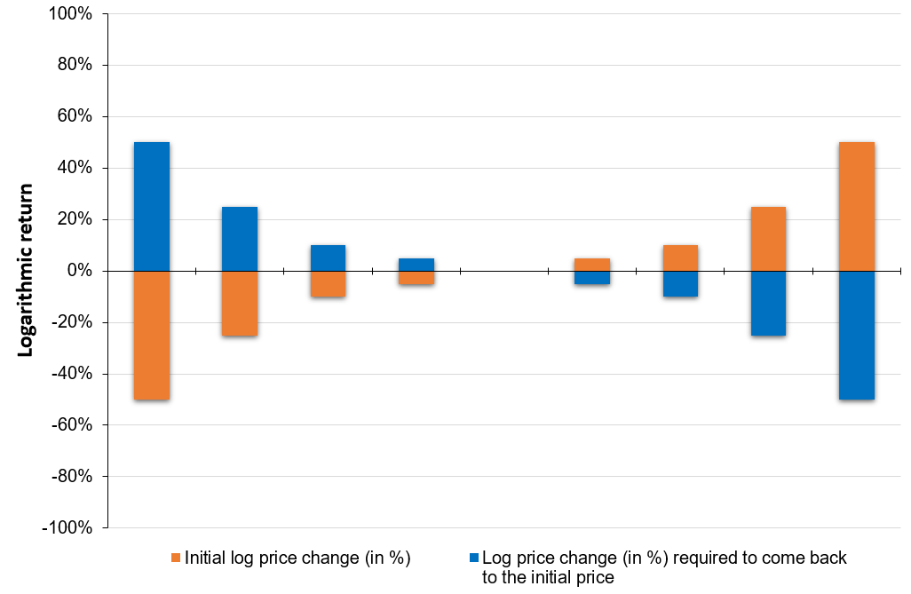
Source: computation by the author.
You can also download below the Excel file for computation of arithmetic returns and visualise the above price change evolution.

Internal rate of return (IRR)
Internal rate of return (IRR) is the rate at which a project undertaken by the firm break’s even. It is a financial metric used by financial analysts to compute the profitability from an investment and is calculated by equating the initial investment and the discounted value of the future cashflows i.e., making the net present value (NPV) equal to zero. The IRR is the sprecail value of the discount rate which makes the NPV equal to zero.
The IRR for a project can be computed as follows:
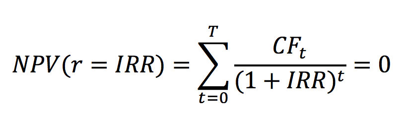
Where,
CFt : Cashflow for time period t
The higher the IRR from a project, the more desirable it is to pursue with the project.
Ex ante and ex post returns
Ex ante and ex post are Latin expressions. Ex ante refers to “before an event” while ex post refers to “after the event”. In context of financial returns, the ex ante return corresponds to prediction or estimation of an asset’s potential future return and can be based on a financial model like the Capital Asset Pricing Model (CAPM). On the other hand, the ex post return corresponds to the actual return generated by an asset historically, and hence are lagging or backward-looking in nature. Ex post returns can be used to forecast ex ante returns for the upcoming period and together, both are used to make sound investment decisions.
Related posts on the SimTrade blog
▶ Jayati WALIA Standard deviation
▶ Raphaël ROERO DE CORTANZE The Internal Rate of Return
▶ Jérémy PAULEN The IRR function in Excel
▶ Léopoldine FOUQUES The IRR, XIRR and MIRR functions in Excel
About the author
The article was written in April 2022 by Jayati WALIA (ESSEC Business School, Grande Ecole Program – Master in Management, 2019-2022).
2 thoughts on “Returns”
Comments are closed.