In this article, Youssef LOURAOUI (Bayes Business School, MSc. Energy, Trade & Finance, 2021-2022) presents the concept of optimal portfolio, which is central in portfolio management.
This article is structured as follows: we first define the notion of an optimal portfolio (in the mean-variance framework) and we then illustrate the concept of optimal portfolio with an example.
Introduction
An investor’s investment portfolio is a collection of assets that he or she possesses. Individual assets such as bonds and equities can be used, as can asset baskets such as mutual funds or exchange-traded funds (ETFs). When constructing a portfolio, investors typically evaluate the expected return as well as the risk. A well-balanced portfolio contains a diverse variety of investments.
An optimal portfolio is a collection of assets that maximizes the trade-off between expected return and risk: the portfolio with the highest expected return for a given level of risk, or the portfolio with the lowest risk for a given level of expected return.
To obtain the optimal portfolio, Markowitz sought to optimize the following dual program:
The first optimization seeks to maximize expected return with respect to a specific level of risk, subject to the short-selling constraint (weights of the portfolio should be equal to one).

The second optimization seeks to minimize the variance of the portfolio with respect to a specific level of expected return, subject to the short-selling constraint (weights of the portfolio should be equal to one).

Mathematical foundations
The investment universe is composed of N assets characterized by their expected returns μ and variance-covariance matrix V. For a given level of expected return μP, the Markowitz model gives the composition of the optimal portfolio. The vector of weights of the optimal portfolio is given by the following formula:
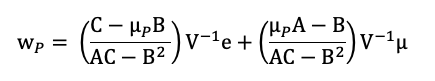
With the following notations:
- wP = vector of asset weights of the portfolio
- μP = desired level of expected return
- e = identity vector
- μ = vector of expected returns
- V = variance-covariance matrix of returns
- V-1 = inverse of the variance-covariance matrix
- t = transpose operation for vectors and matrices
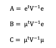
A, B and C are intermediate parameters computed below:
The variance of the optimal portfolio is computed as follows
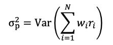
To calculate the standard deviation of the optimal portfolio, we take the square root of the variance.
Optimal portfolio application: the case of two assets
To create the optimal portfolio, we first obtain monthly historical data for the last two years from Bloomberg for two stocks that will comprise our portfolio: Apple and CMS Energy Corporation. Apple is in the technology area, but CMS Energy Corporation is an American company that is entirely in the energy sector. Apple’s historical return for the two years covered was 41.86%, with a volatility of 35.11%. Meanwhile, CMS Energy Corporation’s historical return was 13.95% with a far lower volatility of 15.16%.
According to their risk and return profiles, Apple is an aggressive stock pick in our example, but CMS Energy is a much more defensive stock that would serve as a hedge in our example. The correlation between the two stocks is 0.19, indicating that they move in the same direction. In this example, we will consider the market portfolio, defined as a theoretical portfolio that reflects the return of the whole investment universe, which is captured by the wide US equities index (S&P500 index).
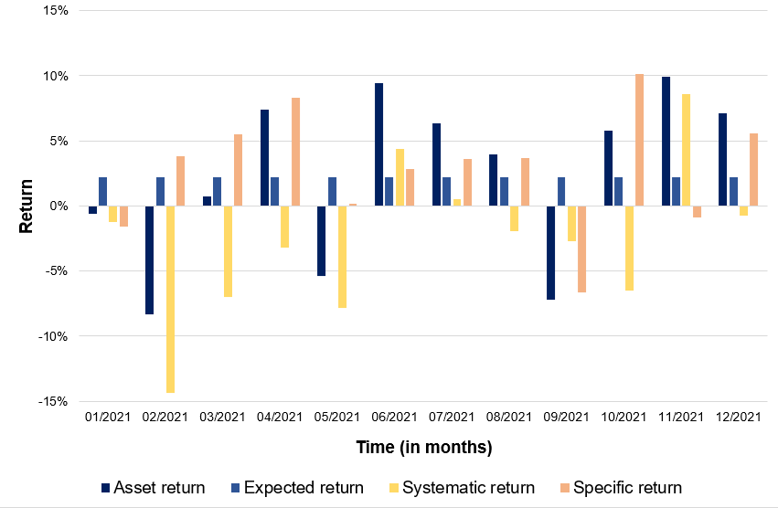
As captured in Figure 1, CMS Energy suffered less severe losses than Apple. When compared to the red bars, the blue bars are far more volatile and sharp in terms of the size of the move in both directions.
Figure 1. Apple and CMS Energy Corporation return breakdown.
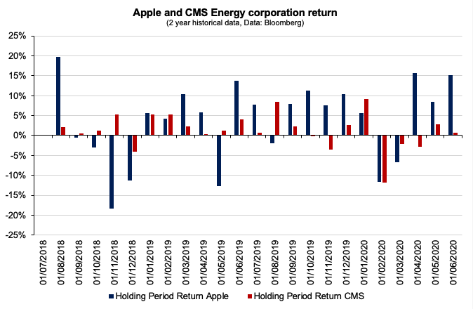
Source: computation by the author (Data: Bloomberg)
After analyzing the historical return on both stocks, as well as their volatility and covariance (and correlation), we can use Mean-Variance portfolio optimization to find the optimal portfolio. According to Markowitz’ foundational study on portfolio construction, the optimal portfolio will attempt to achieve the best risk-return trade-off for an investor. After doing the computations, we discover that the optimal portfolio is composed of 45% Apple stock and 55% CMS Energy corporation stock. This portfolio would return 26.51% with a volatility of 19.23%. As captured in Figure 2, the optimal portfolio is higher on the efficient frontier line and has a higher Sharpe ratio (1.27 vs 1.23 for the theoretical market portfolio).
Figure 2. Optimal portfolio.
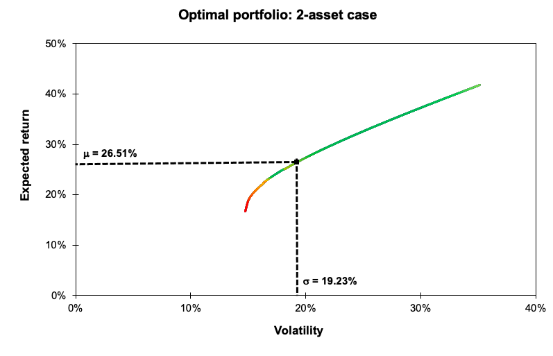
Source: computation by the author (Data: Bloomberg)
You can find below the Excel spreadsheet that complements the example above.

Optimal portfolio application: the general case
We generated a large time series to obtain useful results by downloading the equivalent of 23 years of market data from a data provider (in this example, Bloomberg). We generate the variance-covariance matrix after obtaining all necessary statistical data, which includes the expected return and volatility indicated by the standard deviation of the returns for each stock during the provided period. Table 1 depicts the expected return and volatility for each stock retained in this analysis.
Table 1. Asset characteristics of Apple, Amazon, Microsoft, Goldman Sachs, and Pfizer.
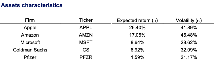
Source: computation by the author.
We can start the optimization task by setting a desirable expected return after computing the expected return, volatility, and the variance-covariance matrix of expected return. With the data that is fed into the appropriate cells, the model will complete the optimization task. For a 20% desired expected return, we get the following results (Table 2).
Table 2. Asset weights for an optimal portfolio.
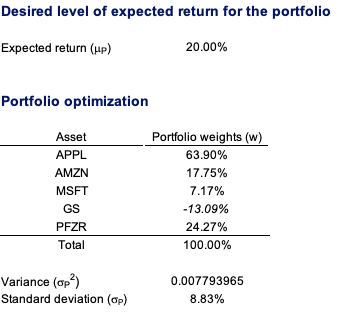
Source: computation by the author.
To demonstrate the effect of diversification in the reduction of volatility, we can form a Markowitz efficient frontier by tilting the desired anticipated return with their relative volatility in a graph. The Markowitz efficient frontier is depicted in Figure 1 for various levels of expected return. We highlighted the portfolio with 20% expected return with its respective volatility in the plot (Figure 3).
Figure 3. Optimal portfolio plot for 5 asset case.
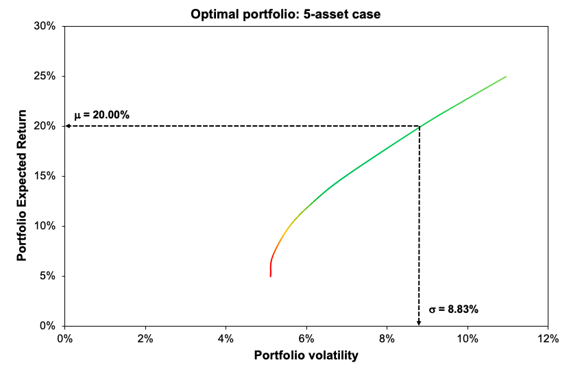
Source: computation by the author.
You can download the Excel file below to use the Markowitz portfolio allocation model.
Why should I be interested in this post?
The purpose of portfolio management is to maximize the (expected) returns on the entire portfolio, not just on one or two stocks. By monitoring and maintaining your investment portfolio, you can build a substantial amount of wealth for a variety of financial goals such as retirement planning. This post facilitates comprehension of the fundamentals underlying portfolio construction and investing.
Related posts on the SimTrade blog
▶ Youssef LOURAOUI Portfolio
▶ Youssef LOURAOUI Factor Investing
▶ Youssef LOURAOUI Origin of factor investing
▶ Youssef LOURAOUI Markowitz Modern Portfolio Theory
Useful resources
Academic research
Pamela, D. and Fabozzi, F., 2010. The Basics of Finance: An Introduction to Financial Markets, Business Finance, and Portfolio Management. John Wiley and Sons Edition.
Markowitz, H., 1952. Portfolio Selection. The Journal of Finance, 7(1): 77-91.
About the author
The article was written in December 2022 by Youssef LOURAOUI (Bayes Business School, MSc. Energy, Trade & Finance, 2021-2022).
 Computation by the author (data: Bloomberg).