In this article, Jayati WALIA (ESSEC Business School, Grande Ecole Program – Master in Management, 2019-2022) presents value at risk.
Introduction
Risk Management is a fundamental pillar of any financial institution to safeguard the investments and hedge against potential losses. The key factor that forms the backbone for any risk management strategy is the measure of those potential losses that an institution is exposed to for any investment. Various risk measures are used for this purpose and Value at Risk (VaR) is the most commonly used risk measure to quantify the level of risk and implement risk management.
VaR is typically defined as the maximum loss which should not be exceeded during a specific time period with a given probability level (or ‘confidence level’). Investments banks, commercial banks and other financial institutions extensively use VaR to determine the level of risk exposure of their investment and calculate the extent of potential losses. Thus, VaR attempts to measure the risk of unexpected changes in prices (or return rates) within a given period.
Mathematically, the VaR corresponds to the quantile of the distribution of returns on the investment.
VaR was not widely used prior to the mid 1990s, although its origin lies further back in time. In the aftermath of events involving the use of derivatives and leverage resulting in disastrous losses in the 1990s (like the failure of Barings bank), financial institutions looked for better comprehensive risk measures that could be implemented. In the last decade, VaR has become the standard measure of risk exposure in financial service firms and has even begun to find acceptance in non-financial service firms.
Computational methods
The three key elements of VaR are the specified level of loss, a fixed period of time over which risk is assessed, and a confidence interval which is essentially the probability of the occurrence of loss-causing event. The VaR can be computed for an individual asset, a portfolio of assets or for the entire financial institution. We detail below the methods used to compute the VaR.
Parametric methods
The most usual parametric method is the variance-covariance method based on the normal distribution.
In this method it is assumed that the price returns for any given asset in the position (and then the position itself) follow a normal distribution. Using the variance-covariance matrix of asset returns and the weights of the assets in the position, we can compute the standard deviation of the position returns denoted as σ. The VaR of the position can then simply computed as a function of the standard deviation and the desired probability level.

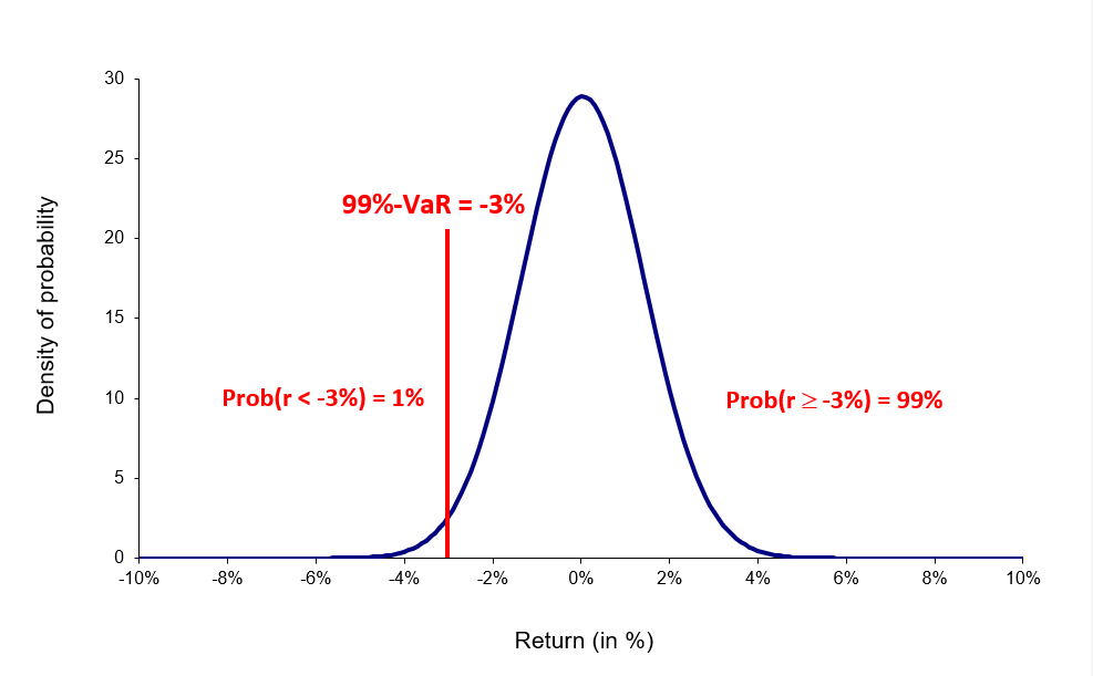
Wherein, p represents the probability used to compute the VaR. For instance, if p is equal to 95%, then the VaR corresponds to the 5% quantile of the distribution of returns. We interpret the VaR as a measure of the loss we observe in 5 out of every 100 trading periods. N-1(x) is the inverse of the cumulative normal distribution function of the confidence level x.
Figure 1. VaR computed with the normal distribution.

For a portfolio with several assets, the standard deviation is computed using the variance-covariance matrix. The expected return on a portfolio of assets is the market-weighted average of the expected returns on the individual assets in the portfolio. For instance, if a portfolio P contains assets A and B with weights wA and wB respectively, the variance of portfolio P’s returns would be:

In the variance-covariance method, the volatility can be computed as the unconditional standard deviation of returns or can be calculated using more sophisticated models to consider the time-varying properties of volatility (like a simple moving average (SMA) or an exponentially weighted moving average (EWMA)).
The historical distribution
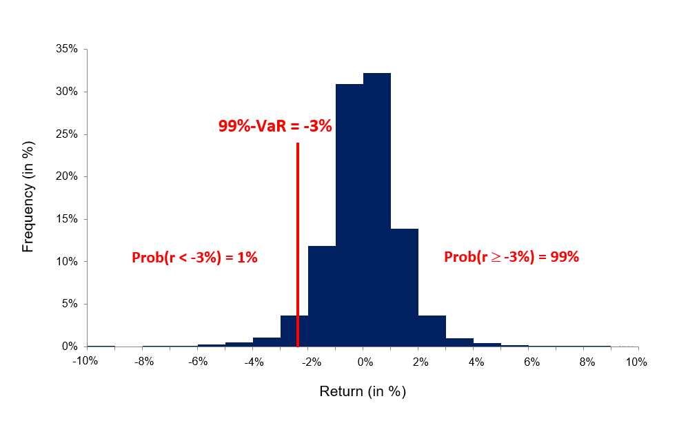
In this method, the historical data of past returns (for say 1,000 daily returns or 4 years of data) are used to build an historical distribution. VaR corresponds to the (1-p) quantile of the historical distribution of returns.
This methodology is based on the approach that the pattern of historical returns is indicative of future returns. VaR is estimated directly from data without estimating any other parameters hence, it is a non-parametric method.
Figure 2. VaR computed with the historical distribution.

Monte Carlo Simulations
This method involves developing a model for generating future price returns and running multiple hypothetical trials through the model. The Monte Carlo simulation is the algorithm through which trials are generated randomly. The computation of VaR is similar to that in historical simulations. The difference only lies in the generation of future return which in case of the historical method is based on empirical data while it is based on simulated data in case of the Monte Carlo method.
The Monte Carlo simulation method is used for complex positions like derivatives where different risk factors (price, volatility, interest rate, dividends, etc.) must be considered.
Limitations of VaR
VaR doesn’t measure worst-case loss
VaR gives a percentage of loss that can be faced in a given confidence level, but it does not tell us about the amount of loss that can be incurred beyond the confidence level.
VaR is not additive
The combined VaR of two different portfolios may be higher than the sum of their individual VaRs.
VaR is only as good as its assumptions and input parameters
In VaR calculations especially parametric methods, unrealistic or inaccurate inputs can give misleading results for VaR. For instance, using the variance-covariance VaR method by assuming normal distribution of returns for assets and portfolios with non-normal skewness.
Different methods give different results
There are many approaches that have been defined over the years to estimate VaR. However, it essential to be careful in choosing the methodology keeping in mind the situation and characteristics of the portfolio or asset into consideration as different methods may be more accurate for specific scenarios.
Related posts on the SimTrade blog
▶ Jayati WALIA The variance-covariance method for VaR calculation
▶ Jayati WALIA The historical method for VaR calculation
▶ Jayati WALIA The Monte Carlo simulation method for VaR calculation
▶ Akshit GUPTA Analysis of the Margin Call movie
Useful Resources
Academic research articles
Artzner, P., F. Delbaen, J.-M. Eber, and D. Heath, (1999) Coherent Measures of Risk, Mathematical Finance, 9, 203-228.
Jorion P. (1997) “Value at Risk: The New Benchmark for Controlling Market Risk,” Chicago: The McGraw-Hill Company.
Longin F. (2000) From VaR to stress testing: the extreme value approach Journal of Banking and Finance, N°24, pp 1097-1130.
Longin F. (2016) Extreme events in finance: a handbook of extreme value theory and its applications Wiley Editions.
Longin F. (2001) Beyond the VaR Journal of Derivatives, 8, 36-48.
About the author
The article was written in September 2021 by Jayati WALIA (ESSEC Business School, Grande Ecole Program – Master in Management, 2019-2022).


2 thoughts on “Value at Risk”
Comments are closed.