

In this article, Youssef LOURAOUI (Bayes Business School, MSc. Energy, Trade & Finance, 2021-2022) presents the systematic risk and specific risk of financial assets, two fundamental concepts in asset pricing models and investment management theories more generally.
This article is structured as follows: we introduce the concept of systematic and specific risk. We then explain the mathematical foundation of this concept. We finish with an insight that sheds light on the relationship between diversification and risk reduction.
Portfolio Theory and Risk
Markowitz (1952) and Sharpe (1964) developed a framework on risk based on their significant work in portfolio theory and capital market theory. All rational profit-maximizing investors seek to possess a diversified portfolio of risky assets, and they borrow or lend to get to a risk level that is compatible with their risk preferences under a set of assumptions. They demonstrated that the key risk measure for an individual asset is its covariance with the market portfolio under these circumstances (the beta).
The fraction of an individual asset’s total variance attributable to the variability of the total market portfolio is referred to as systematic risk, which is assessed by the asset’s covariance with the market portfolio. In the article systematic risk, we develop the economic sources of systematic risk: interest rate risk, inflation risk, exchange rate risk, geopolitical risk, and natural risk.
Additionally, due to the asset’s unique characteristics, an individual asset exhibits variance that is unrelated to the market portfolio (the asset’s non-market variance). Specific risk is the term for non-market variance, and it is often seen as minor because it can be eliminated in a large diversified portfolio. In the article specific risk, we develop the economic sources of specific risk: business risk and financial risk.
Mathematical foundations
Following the Capital Asset Pricing Model (CAPM), the return on asset i, denoted by Ri can be decomposed as
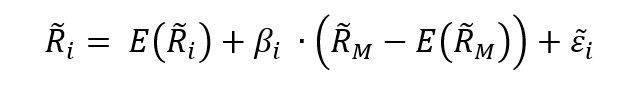
Where:
- Ri the return of asset i
- E(Ri) the expected return of asset i
- βi the measure of the risk of asset i
- RM the return of the market
- E(RM) the expected return of the market
- RM – E(RM) the market factor
- εi the specific part of the return of asset i
The three components of the decomposition are the expected return, the market factor and an idiosyncratic component related to asset only. As the expected return is known over the period, there are only two sources of risk: systematic risk (related to the market factor) and specific risk (related to the idiosyncratic component).
The beta of the asset with the market is computed as:
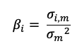
Where:
- σi,m : the covariance of the asset return with the market return
- σm2 : the variance of market return
Total risk can be deconstructed into two main blocks:

The total risk of the asset measured by the variance of asset returns can be computed as:
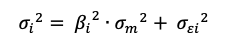
Where:
- βi2 * σm2 = systematic risk
- σεi2 = specific risk
In this decomposition of the total variance, the first component corresponds to the systematic risk and the second component to the specific risk.
Effect of diversification on portfolio risk
Diversification’s objective is to reduce the portfolio’s standard deviation. This assumes an imperfect correlation between securities. Ideally, as investors add securities, the portfolio’s average covariance decreases. How many securities must be included to create a portfolio that is completely diversified? To determine the answer, investors must observe what happens as the portfolio’s sample size increases by adding securities with some positive correlation. Figure 1 illustrates the effect of diversification on portfolio risk, more precisely on total risk and its two components (systematic risk and specific risk).
Figure 1. Effect of diversification on portfolio risk
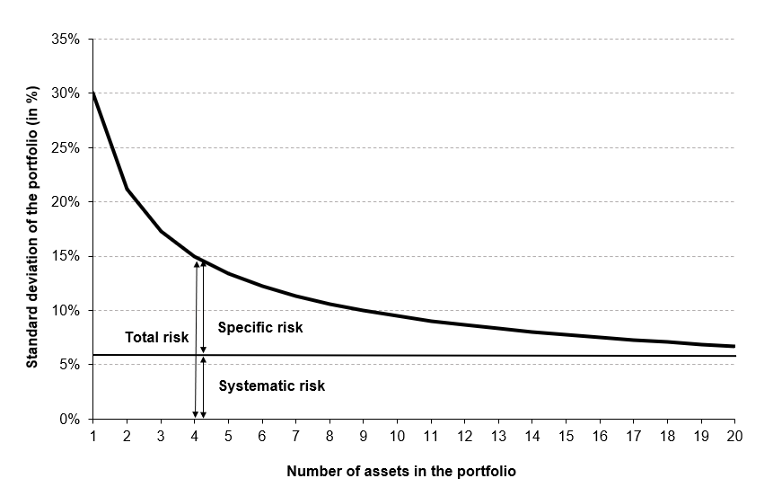
Source: Computations from the author.
The critical point is that by adding stocks that are not perfectly correlated with those already held, investors can reduce the portfolio’s overall standard deviation, which will eventually equal that of the market portfolio. At that point, investors eliminated all specific risk but retained market or systematic risk. There is no way to completely eliminate the volatility and uncertainty associated with macroeconomic factors that affect all risky assets. Additionally, investors can reduce systematic risk by diversifying globally rather than just within the United States, as some systematic risk factors in the United States market (for example, US monetary policy) are not perfectly correlated with systematic risk variables in other countries such as Germany and Japan. As a result, global diversification eventually reduces risk to a global systematic risk level.
You can download below two Excel files which illustrate the effect of diversification on portfolio risk.
The first Excel file deals with the case of independent assets with the same profile (risk and expected return).

Figure 2 depicts the risk reduction of total risk in as we increase the number of assets in the portfolio. We manage to reduce half of the overall portfolio volatility by adding five assets to the portfolio. However, the decrease becomes more and more marginal as we add more assets.
Figure 2. Risk reduction of the portfolio.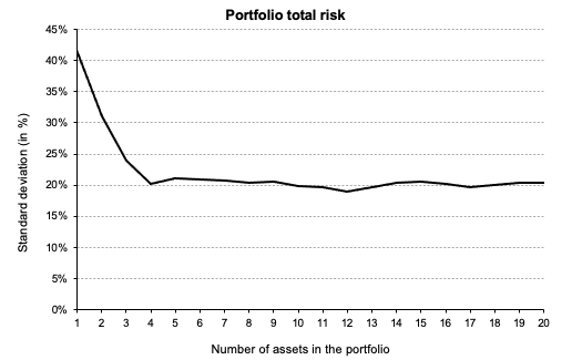 Source: Computations from the author.
Figure 3 depicts the overall risk reduction of a portfolio. The benefit of diversification are more evident when we add the first 5 assets in the portfolio. As depicted in Figure 2, the diversification starts to fade at a certain point as we keep adding more assets in the portfolio. It can be seen in this figure how the specific risk is considerably reduced as we add more assets because of the effect of diversification. Systematic risk (market risk) is more constant and doesn’t change drastically as we diversify the portfolio. Overall, we can clearly see that diversification helps decrease the total risk of a portfolio considerably.
Figure 3. Risk decomposition of the portfolio.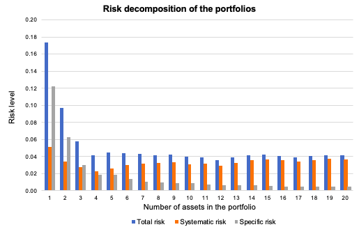 Source: Computations from the author.
The second Excel file deals with the case of dependent assets with the different characteristics (expected return, volatility, and market beta).
Academic research
A series of studies examined the average standard deviation for a variety of portfolios of randomly chosen stocks with varying sample sizes. Evans and Archer (1968) and Tole (1982) calculated the standard deviation for portfolios up to a maximum of twenty stocks. The results indicated that the majority of the benefits of diversification were obtained relatively quickly, with approximately 90% of the maximum benefit of diversification being obtained from portfolios of 12 to 18 stocks. Figure 1 illustrates this effect graphically.
This finding has been modified in two subsequent studies. Statman (1987) examined the trade-off between diversification benefits and the additional transaction costs associated with portfolio expansion. He concluded that a portfolio that is sufficiently diversified should contain at least 30–40 stocks. Campbell, Lettau, Malkiel, and Xu (2001) demonstrated that as the idiosyncratic component of an individual stock’s total risk (specific risk) has increased in recent years, it now requires a portfolio to contain more stocks to achieve the same level of diversification. For example, they demonstrated that the level of diversification possible in the 1960s with only 20 stocks would require approximately 50 stocks by the late 1990s (Reilly and Brown, 2012).
Figure 4. Effect of diversification on portfolio risk 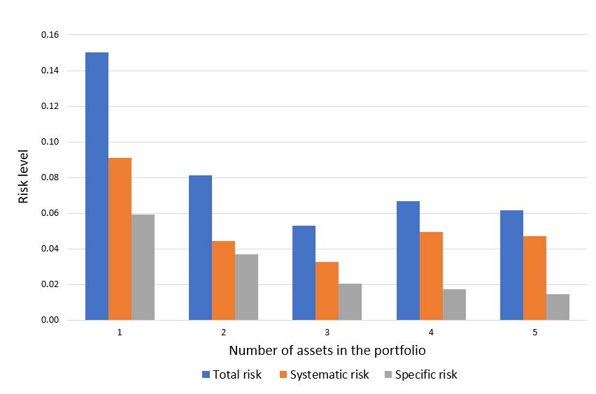 Source: Computation from the author.
You can download below the Excel file which illustrates the effect of diversification on portfolio risk with real assets (Apple, Microsoft, Amazon, etc.). The effect of diversification on the total risk of the portfolio is already significant with the addition of few stocks.
We can appreciate the decomposition of total risk in the below figure with real asset. We can appreciate how asset with low beta had the lowest systematic out of the sample analyzed (i.e. Pfizer). For the whole sample, specific risk is a major concern which makes the major component of risk of each stock. This can be mitigated by holding a well-diversified portfolio that can mitigate this component of risk. Figure 5 depicts the decomposition of total risk for assets (Apple, Microsoft, Amazon, Goldman Sachs and Pfizer).
Figure 5. Decomposition of total risk 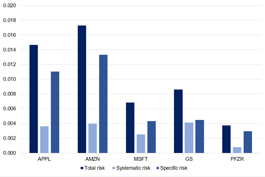 Source: Computation from the author.
You can download below the Excel file which deconstructs the risk of assets (Apple, Microsoft, Amazon, Goldman Sachs, and Pfizer).
Why should I be interested in this post?
If you’re an investor, understanding the source of risk is essential in order to build balanced portfolios that can withstand market corrections and downturns.
If you are a business school or university undergraduate or graduate student, this content will help you in broadening your knowledge of finance.
Related posts on the SimTrade blog
▶ Youssef LOURAOUI Systematic risk
▶ Youssef LOURAOUI Specific risk
▶ Youssef LOURAOUI Beta
▶ Youssef LOURAOUI Portfolio
▶ Youssef LOURAOUI Markowitz Modern Portfolio Theory
▶ Jayati WALIA Capital Asset Pricing Model (CAPM)
Useful resources
Academic research
Campbell, J.Y., Lettau, M., Malkiel, B.G. and Xu, Y. 2001. Have Individual Stocks Become More Volatile? An Empirical Exploration of Idiosyncratic Risk. The Journal of Finance, 56: 1-43.
Evans, J.L., Archer, S.H. 1968. Diversification and the Reduction of Dispersion: An Empirical Analysis. The Journal of Finance, 23(5): 761–767.
Markowitz, H. 1952. Portfolio Selection. The Journal of Finance, 7(1): 77-91.
Mossin, J. 1966. Equilibrium in a Capital Asset Market. Econometrica, 34(4): 768-783.
Reilly, R.K., Brown C.K. 2012. Investment Analysis & Portfolio Management, Tenth Edition. 239-245.
Sharpe, W.F. 1963. A Simplified Model for Portfolio Analysis. Management Science, 9(2): 277-293.
Sharpe, W.F. 1964. Capital Asset Prices: A Theory of Market Equilibrium under Conditions of Risk. The Journal of Finance, 19(3): 425-442.
Statman, M. 1987. How Many Stocks Make a Diversified Portfolio?. The Journal of Financial and Quantitative Analysis, 22(3), 353–363.
Tole T.M. 1982. You can’t diversify without diversifying. The Journal of Portfolio Management. Jan 1982, 8 (2) 5-11.
About the author
The article was written in November 2021 by Youssef LOURAOUI (Bayes Business School, MSc. Energy, Trade & Finance, 2021-2022).