Arbitrage Pricing Theory (APT)

In this article, Youssef LOURAOUI (Bayes Business School, MSc. Energy, Trade & Finance, 2021-2022) presents the concept of arbitrage portfolio, a pillar concept in asset pricing theory.
This article is structured as follows: we present an introduction for the notion of arbitrage portfolio in the context of asset pricing, we present the assumptions and the mathematical foundation of the model and we then illustrate a practical example to complement this post.
Introduction
Arbitrage pricing theory (APT) is a method of explaining asset or portfolio returns that differs from the capital asset pricing model (CAPM). It was created in the 1970s by economist Stephen Ross. Because of its simpler assumptions, arbitrage pricing theory has risen in favor over the years. However, arbitrage pricing theory is far more difficult to apply in practice since it requires a large amount of data and complicated statistical analysis.The following points should be kept in mind when understanding this model:
- Arbitrage is the technique of buying and selling the same item at two different prices at the same time for a risk-free profit.
- Arbitrage pricing theory (APT) in financial economics assumes that market inefficiencies emerge from time to time but are prevented from occurring by the efforts of arbitrageurs who discover and instantly remove such opportunities as they appear.
- APT is formalized through the use of a multi-factor formula that relates the linear relationship between the expected return on an asset and numerous macroeconomic variables.
The concept that mispriced assets can generate short-term, risk-free profit opportunities is inherent in the arbitrage pricing theory. APT varies from the more traditional CAPM in that it employs only one factor. The APT, like the CAPM, assumes that a factor model can accurately characterize the relationship between risk and return.
Assumptions of the APT model
Arbitrage pricing theory, unlike the capital asset pricing model, does not require that investors have efficient portfolios. However, the theory is guided by three underlying assumptions:
- Systematic factors explain asset returns.
- Diversification allows investors to create a portfolio of assets that eliminates specific risk.
- There are no arbitrage opportunities among well-diversified investments. If arbitrage opportunities exist, they will be taken advantage of by investors.
To have a better grasp on the asset pricing theory behind this model, we can recall in the following part the foundation of the CAPM as a complementary explanation for this article.
Capital Asset Pricing Model (CAPM)
William Sharpe, John Lintner, and Jan Mossin separately developed a key capital market theory based on Markowitz’s work: the Capital Asset Pricing Model (CAPM). The CAPM was a huge evolutionary step forward in capital market equilibrium theory, since it enabled investors to appropriately value assets in terms of systematic risk, defined as the market risk which cannot be neutralized by the effect of diversification. In their derivation of the CAPM, Sharpe, Mossin and Litner made significant contributions to the concepts of the Efficient Frontier and Capital Market Line. The seminal contributions of Sharpe, Litner and Mossin would later earn them the Nobel Prize in Economics in 1990.
The CAPM is based on a set of market structure and investor hypotheses:
- There are no intermediaries
- There are no limits (short selling is possible)
- Supply and demand are in balance
- There are no transaction costs
- An investor’s portfolio value is maximized by maximizing the mean associated with projected returns while reducing risk variance
- Investors have simultaneous access to information in order to implement their investment plans
- Investors are seen as “rational” and “risk averse”.
Under this framework, the expected return of a given asset is related to its risk measured by the beta and the market risk premium:
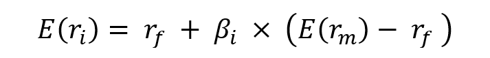
Where :
- E(ri) represents the expected return of asset i
- rf the risk-free rate
- βi the measure of the risk of asset i
- E(rm) the expected return of the market
- E(rm)- rf the market risk premium.
In this model, the beta (β) parameter is a key parameter and is defined as:
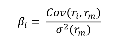
Where:
- Cov(ri, rm) represents the covariance of the return of asset i with the return of the market
- σ2(rm) is the variance of the return of the market.
The beta is a measure of how sensitive an asset is to market swings. This risk indicator aids investors in predicting the fluctuations of their asset in relation to the wider market. It compares the volatility of an asset to the systematic risk that exists in the market. The beta is a statistical term that denotes the slope of a line formed by a regression of data points comparing stock returns to market returns. It aids investors in understanding how the asset moves in relation to the market. According to Fama and French (2004), there are two ways to interpret the beta employed in the CAPM:
- According to the CAPM formula, beta may be thought in mathematical terms as the slope of the regression between the asset return and the market return. Thus, beta quantifies the asset sensitivity to changes in the market return.
- According to the beta formula, it may be understood as the risk that each dollar invested in an asset adds to the market portfolio. This is an economic explanation based on the observation that the market portfolio’s risk (measured by σ2(rm)) is a weighted average of the covariance risks associated with the assets in the market portfolio, making beta a measure of the covariance risk associated with an asset in comparison to the variance of the market return.
Mathematical foundations
The APT can be described formally by the following equation
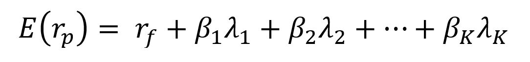
Where
- E(rp) represents the expected return of portfolio p
- rf the risk-free rate
- βk the sensitivity of the return on portfolio p to the kth factor (fk)
- λk the risk premium for the kth factor (fk)
- K the number of risk factors
Richard Roll and Stephen Ross found out that the APT can be sensible to the following factors:
- Expectations on inflation
- Industrial production (GDP)
- Risk premiums
- Term structure of interest rates
Furthermore, the researchers claim that an asset will have varied sensitivity to the elements indicated above, even if it has the same market factor as described by the CAPM.
Application
For this specific example, we want to understand the asset price behavior of two equity indexes (Nasdaq for the US and Nikkei for Japan) and assess their sensitivity to different macroeconomic factors. We extract a time series for Nasdaq equity index prices, Nikkei equity index prices, USD/CHY FX spot rate and US term structure of interest rate (10y-2y yield spread) from the FRED Economics website, a reliable source for macroeconomic data for the last two decades.
The first factor, which is the USD/CHY (US Dollar/Chinese Renminbi Yuan) exchange rate, is retained as the primary factor to explain portfolio return. Given China’s position as a major economic player and one of the most important markets for the US and Japanese corporations, analyzing the sensitivity of US and Japanese equity returns to changes in the USD/CHY Fx spot rate can help in understanding the market dynamics underlying the US and Japanese equity performance. For instance, Texas Instrument, which operates in the sector of electronics and semiconductors, and Nike both have significant ties to the Chinese market, with an overall exposure representing approximately 55% and 18%, respectively (Barrons, 2022). In the example of Japan, in 2017 the Japanese government invested 117 billion dollars in direct investment in northern China, one of the largest foreign investments in China. Similarly, large Japanese listed businesses get approximately 18% of their international revenues from the Chinese market (The Economist, 2019).
The second factor, which is the 10y-2y yield spread, is linked to the shape of the yield curve. A yield curve that is inverted indicates that long-term interest rates are lower than short-term interest rates. The yield on an inverted yield curve decreases as the maturity date approaches. The inverted yield curve, also known as a negative yield curve, has historically been a reliable indicator of a recession. Analysts frequently condense yield curve signals to the difference between two maturities. According to the paper of Yu et al. (2017), there is a significant link between the effects of varying degrees of yield slope with the performance of US equities between 2006 and 2012. Regardless of market capitalization, the impact of the higher yield slope on stock prices was positive.
The APT applied to this example can be described formally by the following equation:

Where
- E(rp) represents the expected return of portfolio p
- rf the risk-free rate
- βp, Chinese FX the sensitivity of the return on portfolio p to the USD/CHY FX spot rate
- βp, US spread the sensitivity of the return on portfolio p to the US term structure
- λChinese FX the risk premium for the FX risk factor
- λUS spread the risk premium for the interest rate risk factor
We run a first regression of the Nikkei Japanese equity index returns onto the macroeconomic variables retained in this analysis. We can highlight the following: Both factors are not statistically significant at a 10% significance level, indicating that the factors have poor predictive power in explaining Nikkei 225 returns over the last two decades. The model has a low R2, equivalent to 0.48%, which indicates that only 0.48% of the behavior of Nikkei performance can be attributed to the change in USD/CHY FX spot rate and US term structure of the yield curve (Table 1).
Table 1. Nikkei 225 equity index regression output.
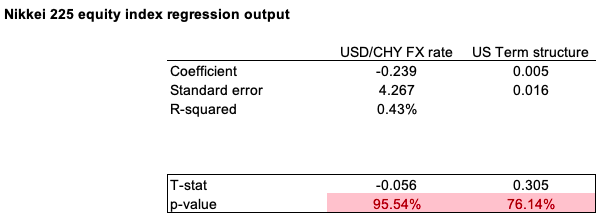
Source: computation by the author (Data: FRED Economics)
Figure 1 and 2 captures the linear relationship between the USD/CHY FX spot rate and the US term structure with respect to the Nikkei equity index.
Figure 1. Relationship between the USD/CHY FX spot rate with respect to the Nikkei 225 equity index.
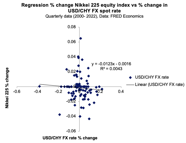
Source: computation by the author (Data: FRED Economics)
Figure 2. Relationship between the US term structure with respect to the Nikkei 225 equity index.
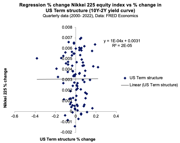
Source: computation by the author (Data: FRED Economics)
We conduct a second regression of the Nasdaq US equity index returns on the retained macroeconomic variables. We may emphasize the following: Both factors are not statistically significant at a 10% significance level, indicating that they have a limited ability to predict Nasdaq returns during the past two decades. The model has a low R2 of 4.45%, indicating that only 4.45% of the performance of the Nasdaq can be attributable to the change in the USD/CHY FX spot rate and the US term structure of the yield curve (Table 2).
Table 2. Nasdaq equity index regression output.
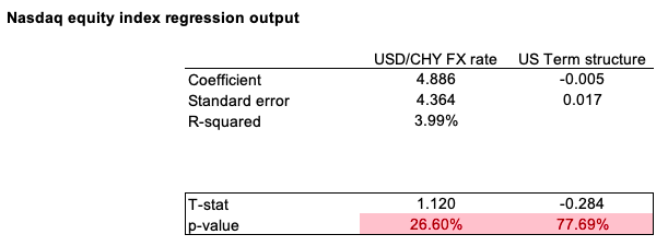
Source: computation by the author (Data: FRED Economics)
Figure 3 and 4 captures the linear relationship between the USD/CHY FX spot rate and the US term structure with respect to the Nasdaq equity index.
Figure 3. Relationship between the USD/CHY FX spot rate with respect to the Nasdaq equity index.
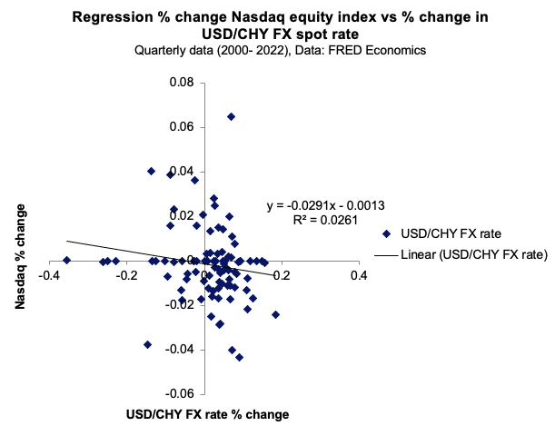
Source: computation by the author (Data: FRED Economics)
Figure 4. Relationship between the US term structure with respect to the Nasdaq equity index.
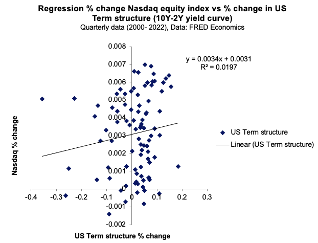
Source: computation by the author (Data: FRED Economics)
Applying APT
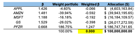
We can create a portfolio with similar factor sensitivities as the Arbitrage Portfolio by combining the first two index portfolios (with a Nasdaq Index weight of 40% and a Nikkei Index weight of 60%). This is referred to as the Constructed Index Portfolio. The Arbitrage portfolio will have a full weighting on US equity index (100% Nasdaq equity index). The Constructed Index Portfolio has the same systematic factor betas as the Arbitrage Portfolio, but has a higher expected return (Table 3).
Table 3. Index, constructed and Arbitrage portfolio return and sensitivity table.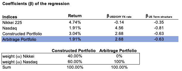
Source: computation by the author (Data: FRED Economics)
As a result, the Arbitrage portfolio is overvalued. We will then buy shares of the Constructed Index Portfolio and use the profits to sell shares of the Arbitrage Portfolio. Because every investor would sell an overvalued portfolio and purchase an undervalued portfolio, any arbitrage profit would be wiped out.
Excel file for the APT application
You can find below the Excel spreadsheet that complements the example above.

Why should I be interested in this post?
In the CAPM, the factor is the market factor representing the global uncertainty of the market. In the late 1970s, the portfolio management industry aimed to capture the market portfolio return, but as financial research advanced and certain significant contributions were made, this gave rise to other factor characteristics to capture some additional performance. Analyzing the historical contributions that underpins factor investing is fundamental in order to have a better understanding of the subject.
Related posts on the SimTrade blog
▶ Jayati WALIA Capital Asset Pricing Model (CAPM)
▶ Youssef LOURAOUI Origin of factor investing
▶ Youssef LOURAOUI Factor Investing
▶ Youssef LOURAOUI Fama-MacBeth regression method: stock and portfolio approach
▶ Youssef LOURAOUI Fama-MacBeth regression method: Analysis of the market factor
▶ Youssef LOURAOUI Fama-MacBeth regression method: N-factors application
▶ Youssef LOURAOUI Portfolio
Useful resources
Academic research
Lintner, J. (1965) The Valuation of Risk Assets and the Selection of Risky Investments in Stock Portfolios and Capital Budgets. The Review of Economics and Statistics 47(1): 13-37.
Lintner, J. (1965) Security Prices, Risk and Maximal Gains from Diversification. The Journal of Finance 20(4): 587-615.
Roll, Richard & Ross, Stephen. (1995). The Arbitrage Pricing Theory Approach to Strategic Portfolio Planning. Financial Analysts Journal 51, 122-131.
Ross, S. (1976) The arbitrage theory of capital asset pricing Journal of Economic Theory 13(3), 341-360.
Sharpe, W.F. (1963) A Simplified Model for Portfolio Analysis. Management Science 9(2): 277-293.
Sharpe, W.F. (1964) Capital Asset Prices: A theory of Market Equilibrium under Conditions of Risk. The Journal of Finance 19(3): 425-442.
Yu, G., P. Fuller, D. Didia (2013) The Impact of Yield Slope on Stock Performance Southwestern Economic Review 40(1): 1-10.
Business Analysis
Barrons (2022) Apple, Nike, and 6 Other Companies With Big Exposure to China.
The Economist (2019) Japan Inc has thrived in China of late.
Time series
FRED Economics (2022) Chinese Yuan Renminbi to U.S. Dollar Spot Exchange Rate (DEXCHUS).
FRED Economics (2022) 10-Year Treasury Constant Maturity Minus 2-Year Treasury Constant Maturity (T10Y2Y).
FRED Economics (2022) NASDAQ Composite Index (NASDAQCOM).
FRED Economics (2022) Nikkei Stock Average, Nikkei 225 (NIKKEI225).
About the author
The article was written in January 2023 by Youssef LOURAOUI (Bayes Business School, MSc. Energy, Trade & Finance, 2021-2022).


 Source: computation by the author (data: Refinitiv Eikon).
 Source: computation by the author (Data: Refinitiv Eikon).
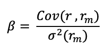
 Source: computation by the author (Data: Bloomberg)
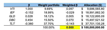 Source: computation by the author. (Data: Reuters Eikon)