

In this article, Jayati WALIA (ESSEC Business School, Grande Ecole Program – Master in Management, 2019-2022) presents the historical method for VaR calculation.
Introduction
A key factor that forms the backbone for risk management is the measure of those potential losses that an institution is exposed to any investment. Various risk measures are used for this purpose and Value at Risk (VaR) is the most commonly used risk measure to quantify the level of risk and implement risk management.
VaR is typically defined as the maximum loss which should not be exceeded during a specific time period with a given probability level (or ‘confidence level’). VaR is used extensively to determine the level of risk exposure of an investment, portfolio or firm and calculate the extent of potential losses. Thus, VaR attempts to measure the risk of unexpected changes in prices (or return rates) within a given period. Mathematically, the VaR corresponds to the quantile of the distribution of returns.
The two key elements of VaR are a fixed period of time (say one or ten days) over which risk is assessed and a confidence level which is essentially the probability of the occurrence of loss-causing event (say 95% or 99%). There are various methods used to compute the VaR. In this post, we discuss in detail the historical method which is a popular way of estimating VaR.
Calculating VaR using the historical method
Historical VaR is a non-parametric method of VaR calculation. This methodology is based on the approach that the pattern of historical returns is indicative of the pattern of future returns.
The first step is to collect data on movements in market variables (such as equity prices, interest rates, commodity prices, etc.) over a long time period. Consider the daily price movements for CAC40 index within the past 2 years (512 trading days). We thus have 512 scenarios or cases that will act as our guide for future performance of the index i.e., the past 512 days will be representative of what will happen tomorrow.
For each day, we calculate the percentage change in price for the CAC40 index that defines our probability distribution for daily gains or losses. We can express the daily rate of returns for the index as:
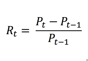
Where Rt represents the (arithmetic) return over the period [t-1, t] and Pt the price at time t (the closing price for daily data). Note that the logarithmic return is sometimes used (see my post on Returns).
Next, we sort the distribution of historical returns in ascending order (basically in order of worst to best returns observed over the period). We can now interpret the VaR for the CAC40 index in one-day time horizon based on a selected confidence level (probability).
Since the historical VaR is estimated directly from data without estimating or assuming any other parameters, hence it is a non-parametric method.
For instance, if we select a confidence level of 99%, then our VaR estimate corresponds to the 1st percentile of the probability distribution of daily returns (the top 1% of worst returns). In other words, there are 99% chances that we will not obtain a loss greater than our VaR estimate (for the 99% confidence level). Similarly, VaR for a 95% confidence level corresponds to top 5% of the worst returns.
Figure 1. Probability distribution of returns for the CAC40 index.
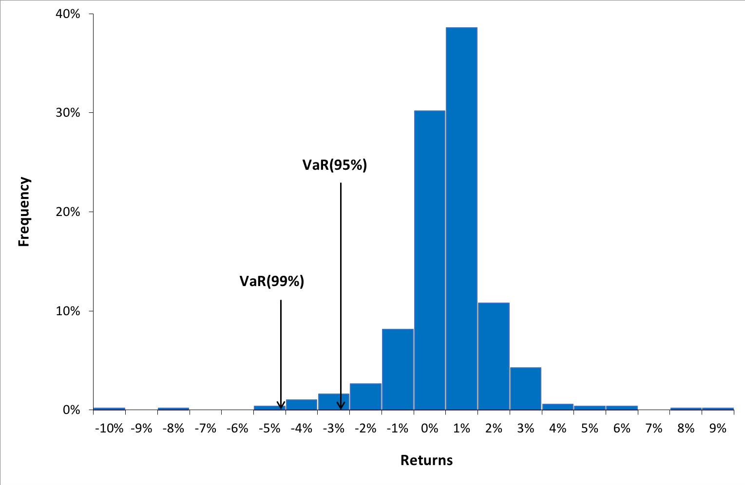
Source: computation by the author (data source: Bloomberg).
You can download below the Excel file for the VaR calculation with the historical method. The historical distribution is estimated with historical data from the CAC 40 index.

From the above graph, we can interpret VaR for 90% confidence level as -3.99% i.e., there is a 90% probability that daily returns we obtain in future are greater than -3.99%. Similarly, VaR for 99% confidence level as -5.60% i.e., there is a 99% probability that daily returns we obtain in future are greater than -5.60%.
Advantages and limitations of the historical method
The historical method is a simple and fast method to calculate VaR. For a portfolio, it eliminates the need to estimate the variance-covariance matrix and simplifies the computations especially in cases of portfolios with a large number of assets. This method is also intuitive. VaR corresponds to a large loss sustained over an historical period that is known. Hence users can go back in time and explain the circumstances behind the VaR measure.
On the other hand, the historical method has a few of drawbacks. The assumption is that the past represents the immediate future is highly unlikely in the real world. Also, if the horizon window omits important events (like stock market booms and crashes), the distribution will not be well represented. Its calculation is only as strong as the number of correct data points measured that fully represent changing market dynamics even capturing crisis events that may have occurred such as the Covid-19 crisis in 2020 or the financial crisis in 2008. In fact, even if the data does capture all possible historical dynamics, it may not be sufficient because market will never entirely replicate past movements. Finally, the method assumes that the distribution is stationary. In practice, there may be significant and predictable time variation in risk.
Related posts on the SimTrade blog
▶ Jayati WALIA Quantitative Risk Management
▶ Jayati WALIA Value at Risk
▶ Jayati WALIA The variance-covariance method for VaR calculation
▶ Jayati WALIA The Monte Carlo simulation method for VaR calculation
Useful resources
Jorion, P. (2007) Value at Risk , Third Edition, Chapter 10 – VaR Methods, 276-279.
Longin F. (2000) From VaR to stress testing : the extreme value approach Journal of Banking and Finance, 24, 1097-1130.
About the author
The article was written in December 2021 by Jayati WALIA (ESSEC Business School, Grande Ecole Program – Master in Management, 2019-2022).