Bitcoin: the mother of all cryptocurrencies

October 26, 2023 by Snehasish CHINARA

Bitcoin: the mother of all cryptocurrencies

In this article, Snehasish CHINARA (ESSEC Business School, Grande Ecole Program – Master in Management, 2022-2024) explains Bitcoin which is considered as the mother of all cryptocurrencies.

Historical context and background

The genesis of Bitcoin can be traced back to the aftermath of the Financial Crisis of 2008, when a growing desire emerged for a currency immune to central authority control. Traditional banks had faltered, leading to the devaluation of money through government-sanctioned printing. The absence of a definitive limit on money creation fostered uncertainty. Bitcoin ingeniously addressed this quandary by establishing a fixed supply of coins and a controlled production rate through transparent coding. This code’s openness ensured that no entity, including governments, could manipulate the currency’s value. Consequently, Bitcoin’s worth became solely determined by market dynamics, evading the arbitrary alterations typical of government-managed currencies.

Furthermore, Bitcoin revolutionized financial transactions by eliminating reliance on third-party intermediaries, exemplified by banks. Users can now engage in direct peer-to-peer transactions, circumventing the potential for intermediaries to engage in risky financial ventures akin to the 2008 Financial Crisis. The process of safeguarding one’s Bitcoins is equally innovative, as users manage their funds through a Bitcoin Wallet. Unlike traditional banks, these wallets operate as personal assets, with users as their own bankers. While various companies offer wallet services, the underlying code remains accessible for review, ensuring customers’ trust and the safety of their deposits.

Bitcoin Logo

Source: internet.

Figure 1. Key Dates in Bitcoin History

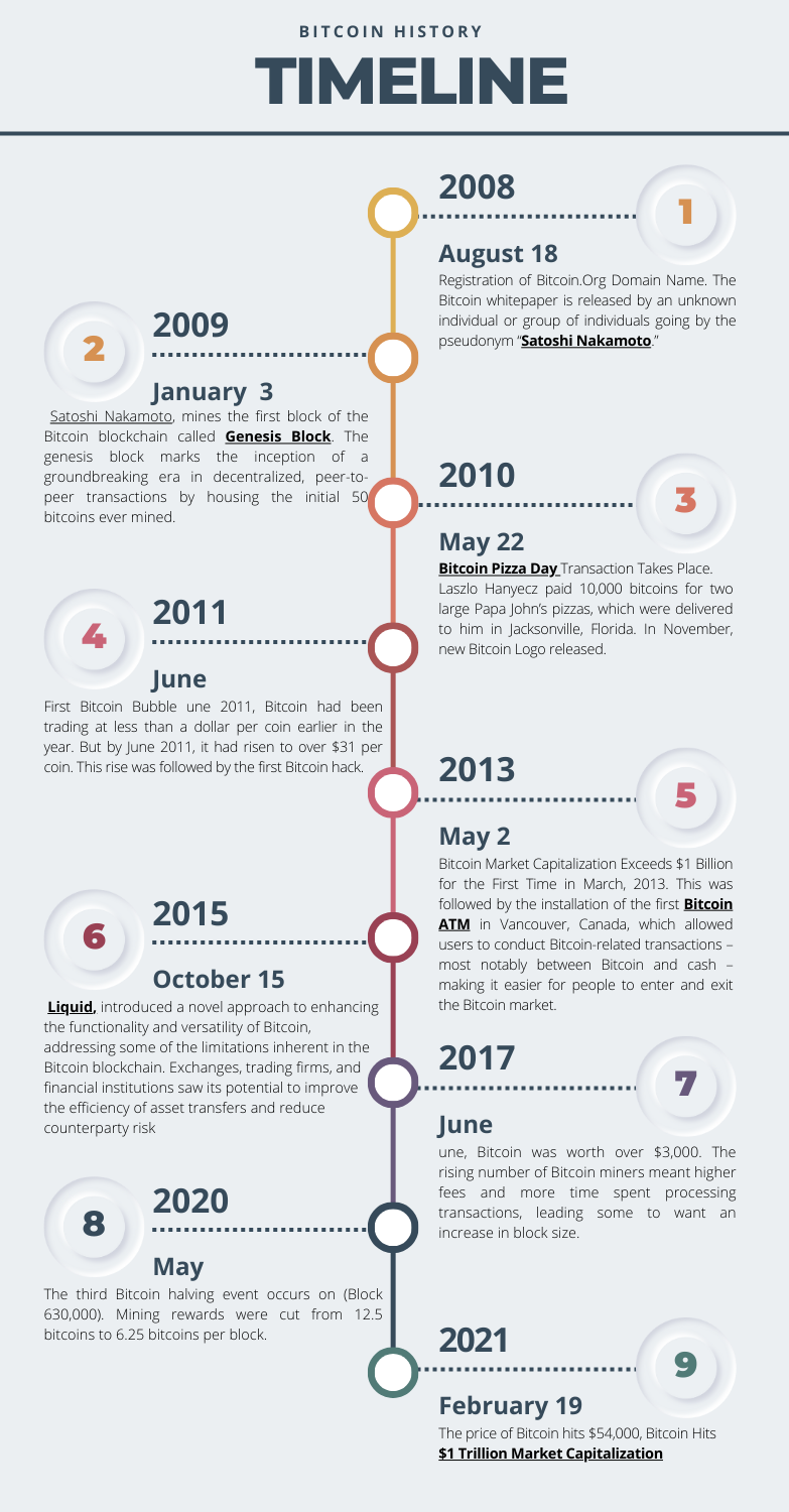
Source: author of this post.

Key features and use cases

Examples of areas where Bitcoin is currently being used:

Digital Currency: Bitcoin serves as a digital currency for everyday transactions, allowing users to buy goods and services online and in physical stores.
Crypto Banking: Bitcoin is used in decentralized finance (DeFi) applications, where users can lend, borrow, and earn interest on their Bitcoin holdings.
Asset Tokenization: Bitcoin is used to tokenize real-world assets like real estate and art, making them more accessible and divisible among investors.
Onchain Governance: Some blockchain projects utilize Bitcoin for on-chain governance, enabling token holders to vote on protocol upgrades and changes.
Smart Contracts: While Ethereum is more widely associated with smart contracts, Bitcoin’s second layer solutions like RSK (Rootstock) allow for the execution of smart contracts on the Bitcoin blockchain.
Corporate Treasuries: Large corporations, such as Tesla, have invested in Bitcoin as a store of value and an asset to diversify their corporate treasuries.
State Treasuries: Some countries, like El Salvador, have adopted Bitcoin as legal tender and added it to their national treasuries to facilitate cross-border remittances and financial inclusion.
Store of Value During Times of Conflict: In regions with economic instability or conflict, Bitcoin is used as a hedge against currency devaluation and asset confiscation.
Online Gambling: Bitcoin is widely accepted in online gambling platforms, providing users with a secure and pseudonymous way to wager on games and sports.
Salary Payments for Freelancers in Emerging Markets: Freelancers in countries with limited access to traditional banking use Bitcoin to receive payments from international clients, circumventing costly and slow remittance services.
Cross-Border Transactions with Bitcoin Gold: Cross-border transactions can often be complex, time-consuming, and costly due to the involvement of multiple intermediaries and the varying regulations of different countries. However, Bitcoin Gold offers a streamlined solution for facilitating global payments, making cross-border transactions more efficient and accessible.

These examples highlight the diverse utility of Bitcoin, ranging from everyday transactions to more complex financial applications and as a tool for economic empowerment in various contexts.

Technology and underlying blockchain

Blockchain technology is the foundational innovation that underpins Bitcoin, the world’s first and most well-known cryptocurrency. At its core, blockchain is a decentralized and distributed ledger system that records transactions across a network of computers in a secure and transparent manner. In the context of Bitcoin, this blockchain serves as a public ledger that tracks every transaction ever made with the cryptocurrency. What sets blockchain apart is its ability to ensure trust and security without the need for a central authority, such as a bank or government. Each block in the chain contains a set of transactions, and these blocks are linked together in a chronological and immutable fashion. This means that once a transaction is recorded on the blockchain, it cannot be altered or deleted. This transparency, immutability, and decentralization make blockchain technology a revolutionary tool not only for digital currencies like Bitcoin but also for a wide range of applications in various industries, from finance and supply chain management to healthcare and beyond.

Moreover, Bitcoin operates on a decentralized network of computers (nodes) worldwide. These nodes validate and confirm transactions, ensuring that the network remains secure, censorship-resistant, and immune to central control. The absence of a central authority is a fundamental characteristic of Bitcoin and a key differentiator from traditional financial systems. Bitcoin relies on a PoW consensus mechanism for securing its network. Miners compete to solve complex mathematical puzzles, and the first one to solve it gets the right to add a new block of transactions to the blockchain. This process ensures the security of the network, prevents double-spending, and maintains the integrity of the ledger. Bitcoin has a fixed supply of 21 million coins, a feature hard-coded into its protocol. The rate at which new Bitcoins are created is reduced by half approximately every four years through a process known as a “halving.” This limited supply is in stark contrast to fiat currencies, which can be printed without restriction.

These technological aspects collectively make Bitcoin a groundbreaking innovation that has disrupted traditional finance and is increasingly studied and integrated into the field of finance. It offers unique opportunities and challenges for finance students to explore, including its impact on monetary policy, investment, and the broader financial ecosystem.

Supply of coins

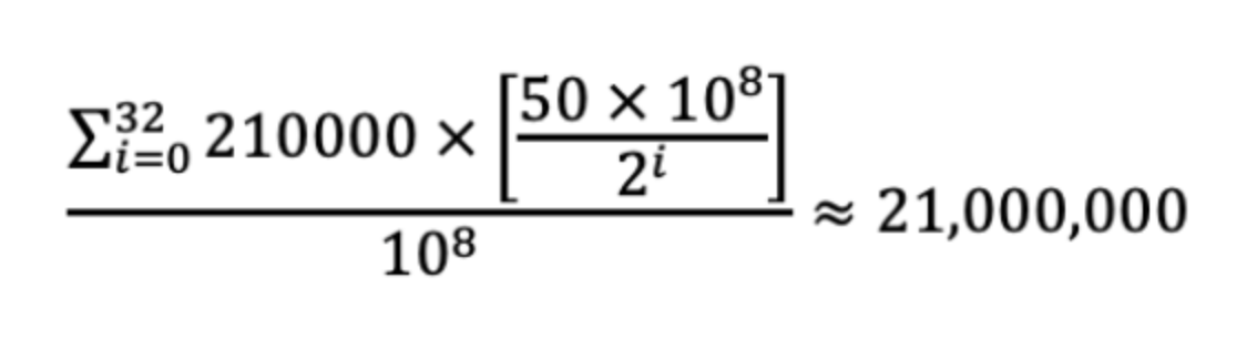
Looking at the supply side of bitcoins, the number of bitcoins in circulation is given by the following mathematical formula:

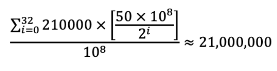
Formula for the number of bitcoins in circulation

This calculation hinges upon the fundamental concept of the Bitcoin supply schedule, which employs a diminishing issuance rate through a process known as “halving”.

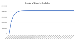
Figure 2 represents the evolution of the number of bitcoins in circulation overt time based on the above formula.

Figure 2. Number of bitcoins in circulation

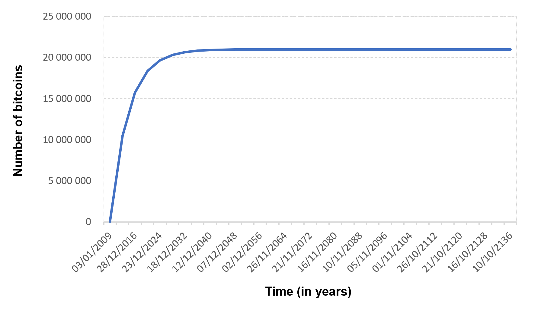
Source: computation by the author.

You can download below the Excel file for the data and the figure of the number of bitcoins in circulation.

Historical data for Bitcoin

How to get the data?

The Bitcoin is the most popular cryptocurrency on the market, and historical data for the Bitcoin such as prices and volume traded can be easily downloaded from the internet sources such as Yahoo! Finance, Blockchain.com & CoinMarketCap. For example, you can download data for Bitcoin on Yahoo! Finance (the Yahoo! code for Bitcoin is BTC-USD).

Figure 4. Bitcoin data

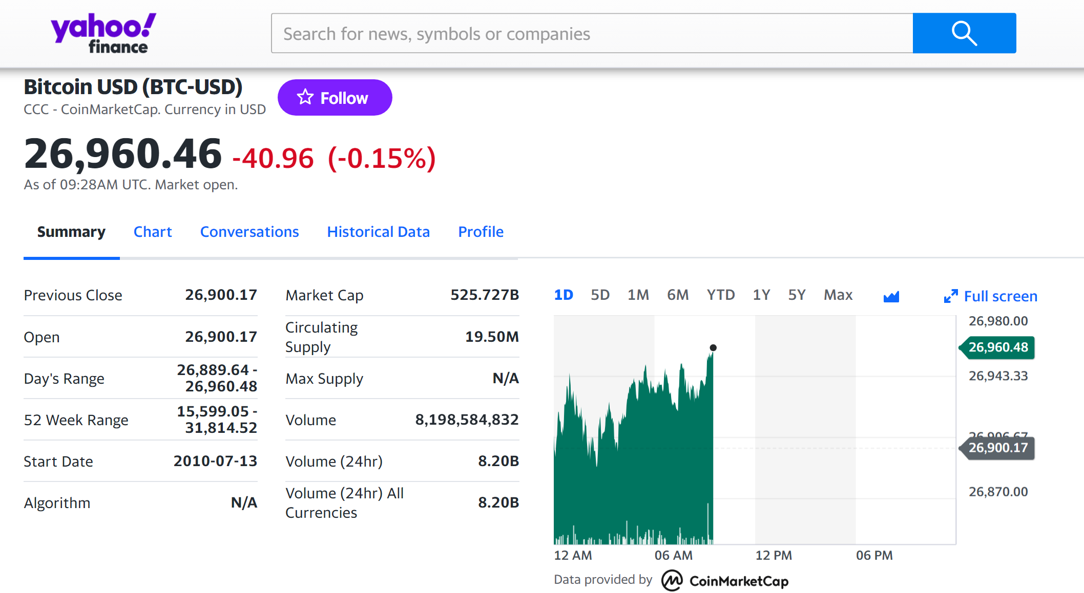
Source: Yahoo! Finance.

Historical data for the Bitcoin market prices

The market price of Bitcoin is a dynamic and intricate element that reflects a multitude of factors, both intrinsic and extrinsic. The gradual rise in market value over time indicates a willingness among investors and traders to offer higher prices for the cryptocurrency. This signifies a rising interest and strong belief in the project’s potential for the future. The market price reflects the collective sentiment of investors and traders. Comparing the market price of Bitcoin to other similar cryptocurrencies or benchmark assets can provide insights into its relative strength and performance within the market.

The value of Bitcoin in the market is influenced by a variety of elements, with each factor contributing uniquely to their pricing. One of the most significant influences is market sentiment and investor psychology. These factors can cause prices to shift based on positive news, regulatory changes, or reactive selling due to fear. Furthermore, the real-world implementations and usages of Bitcoin are crucial for its prosperity. Concrete use cases such as Decentralized Finance (DeFi), Non-Fungible Tokens (NFTs), and international transactions play a vital role in creating demand and propelling price appreciation. Meanwhile, adherence to basic economic principles is evident in the supply-demand dynamics, where scarcity due to limited issuance, halving events, and token burns interact with the balance between supply and demand.

With the number of coins in circulation, the information on the price of coins for a given currency is also important to compute Bitcoin’s market capitalization.

Figure 5 below represents the evolution of the price of Bitcoin in US dollar over the period October 2014 – August 2023. The price corresponds to the “closing” price (observed at 10:00 PM CET at the end of the month).

Figure 5. Evolution of the Bitcoin price

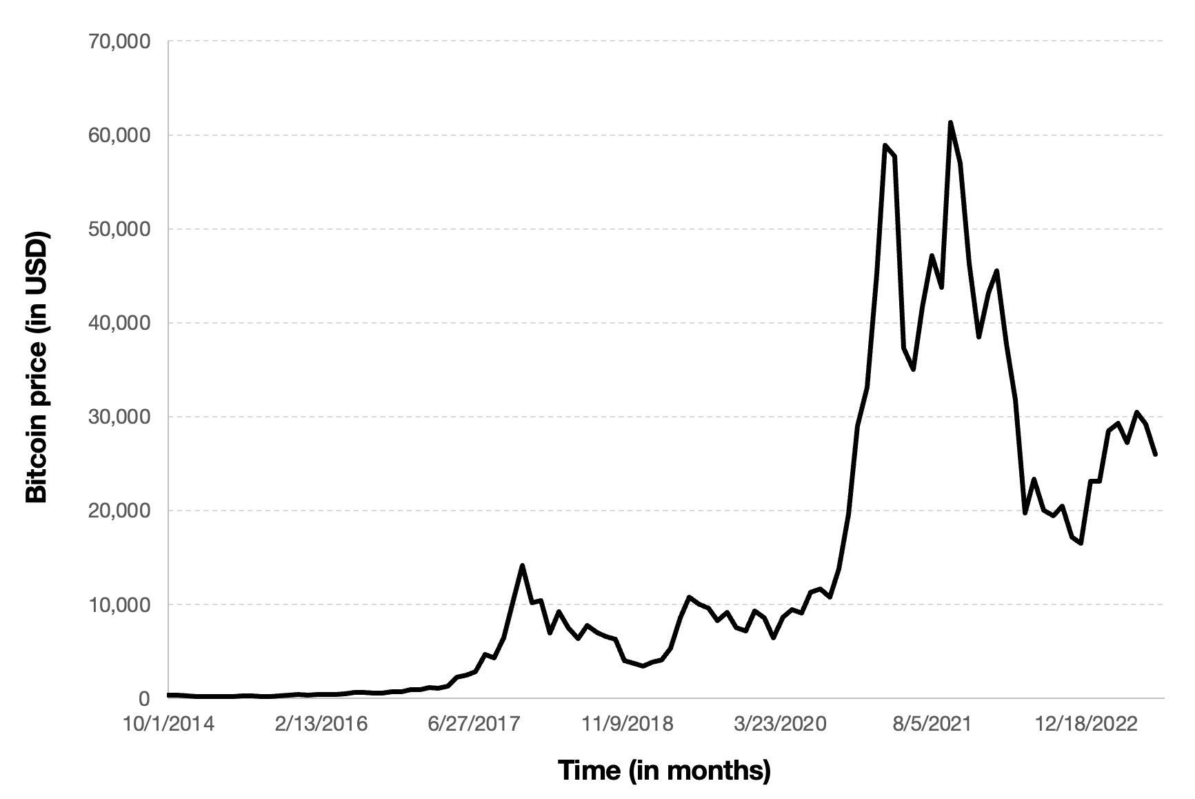
Source: computation by the author (data source: Yahoo! Finance).

Python code

Python script to download Bitcoin historical data and save it to an Excel sheet::

import yfinance as yf
import pandas as pd

# Define the ticker symbol and date range
ticker_symbol = “BTC-USD”
start_date = “2020-01-01”
end_date = “2023-01-01”

# Download historical data using yfinance
data = yf.download(ticker_symbol, start=start_date, end=end_date)

# Create a Pandas DataFrame
df = pd.DataFrame(data)

# Create a Pandas Excel writer object
excel_writer = pd.ExcelWriter(‘bitcoin_historical_data.xlsx’, engine=’openpyxl’)

# Write the DataFrame to an Excel sheet
df.to_excel(excel_writer, sheet_name=’Bitcoin Historical Data’)

# Save the Excel file
excel_writer.save()

print(“Data has been saved to bitcoin_historical_data.xlsx”)

# Make sure you have the required libraries installed and adjust the “start_date” and “end_date” variables to the desired date range for the historical data you want to download.

The code above allows you to download the data from Yahoo! Finance.

R code

The R program below written by Shengyu ZHENG allows you to download the data from Yahoo! Finance website and to compute summary statistics and risk measures about the Bitcoin.

Data file

The R program that you can download above allows you to download the data for the Bitcoin from the Yahoo! Finance website. The database starts on September 17, 2014.

Table 3 below represents the top of the data file for the Bitcoin downloaded from the Yahoo! Finance website with the R program.

Table 3. Top of the data file for the Bitcoin.
Top of the file for the Bitcoin data
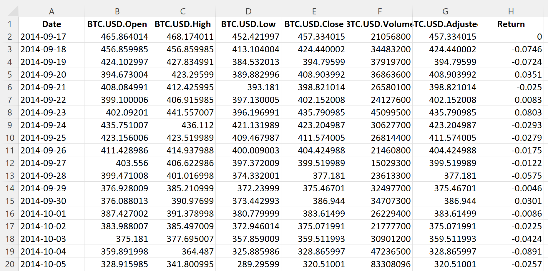
Source: computation by the author (data: Yahoo! Finance website).

Evolution of the Bitcoin

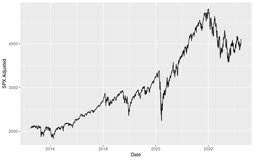
Figure 6 below gives the evolution of the Bitcoin from September 17, 2014 to December 31, 2022 on a daily basis.

Figure 6. Evolution of the Bitcoin.

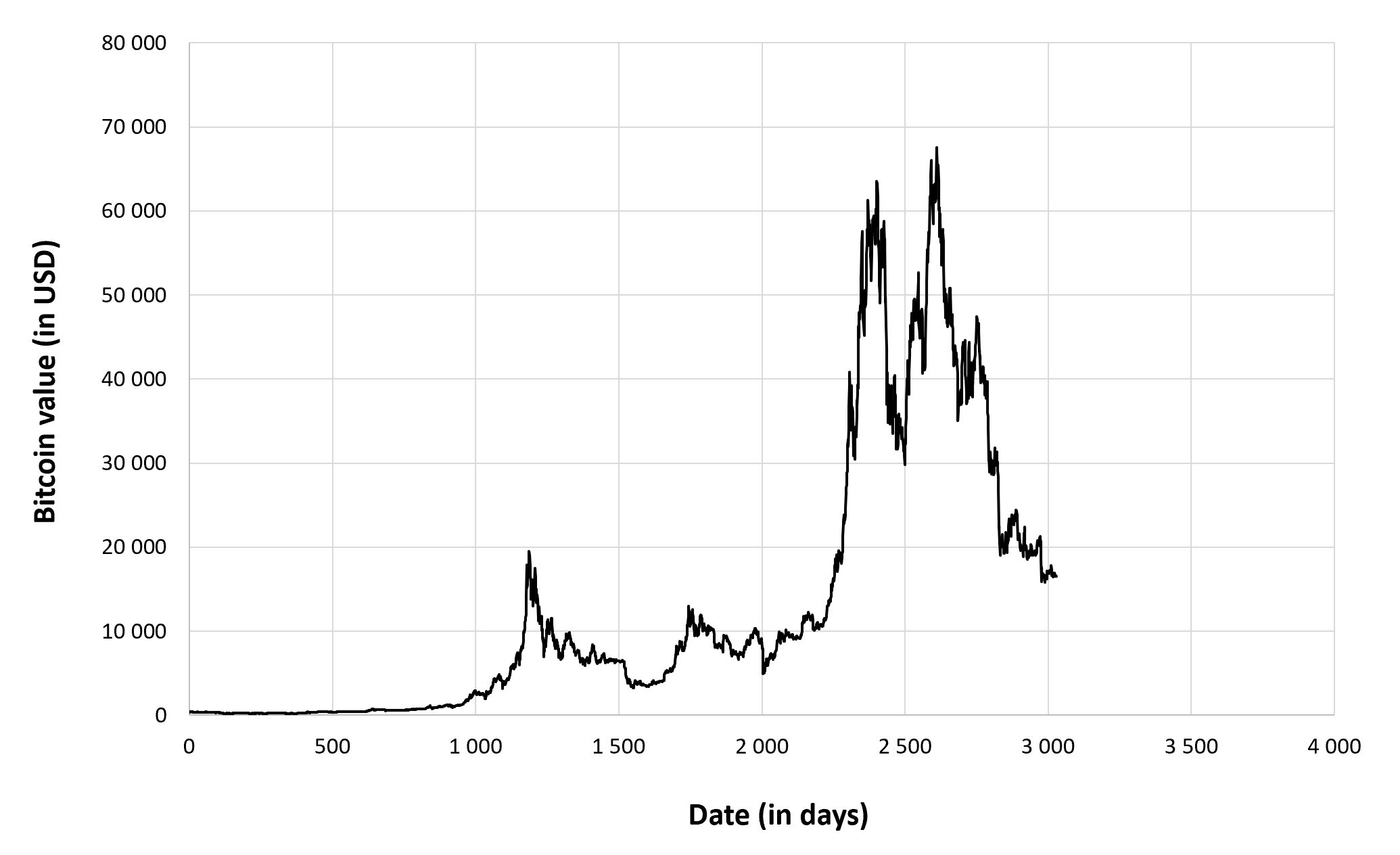
Source: computation by the author (data: Yahoo! Finance website).

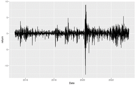
Figure 7 below gives the evolution of the Bitcoin returns from September 17, 2014 to December 31, 2022 on a daily basis.

Figure 7. Evolution of the Bitcoin returns.

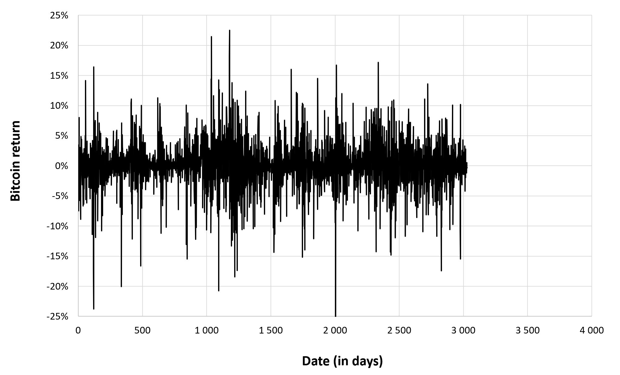
Source: computation by the author (data: Yahoo! Finance website).

Summary statistics for the Bitcoin

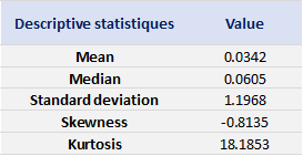
The R program that you can download above also allows you to compute summary statistics about the returns of the Bitcoin.

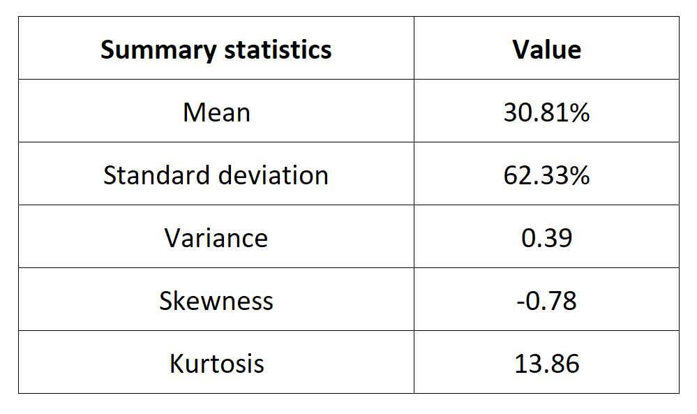
Table 4 below presents the following summary statistics estimated for the Bitcoin:

The mean
The standard deviation (the squared root of the variance)
The skewness
The kurtosis.

The mean, the standard deviation / variance, the skewness, and the kurtosis refer to the first, second, third and fourth moments of statistical distribution of returns respectively.

Table 4. Summary statistics for the Bitcoin.

Source: computation by the author (data: Yahoo! Finance website).

Statistical distribution of the Bitcoin returns

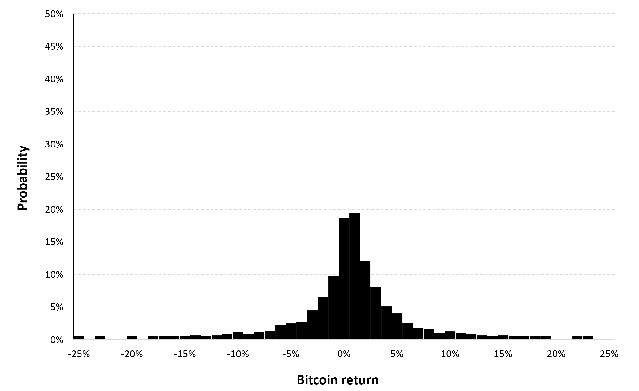
Historical distribution

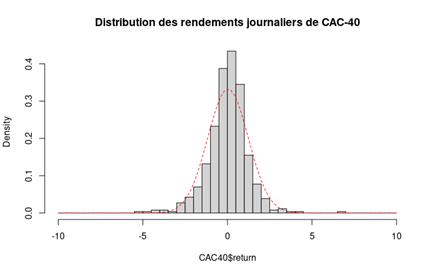
Figure 8 represents the historical distribution of the Bitcoin daily returns for the period from September 17, 2014 to December 31, 2022.

Figure 8. Historical distribution of the Bitcoin returns.

Source: computation by the author (data: Yahoo! Finance website).

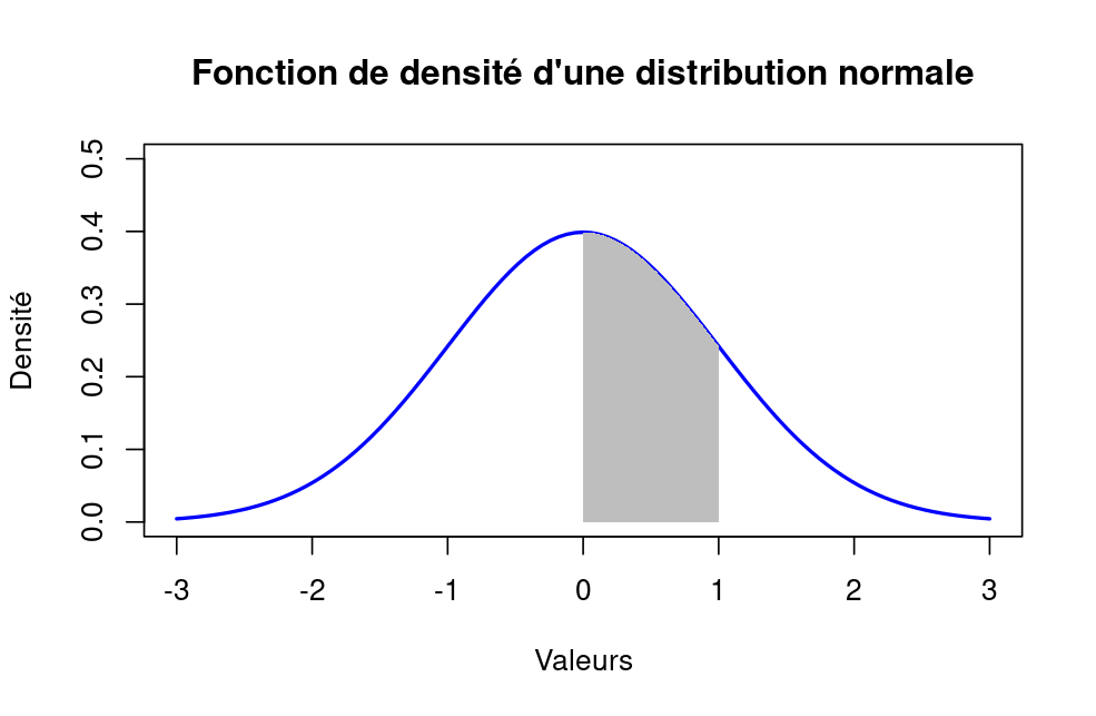
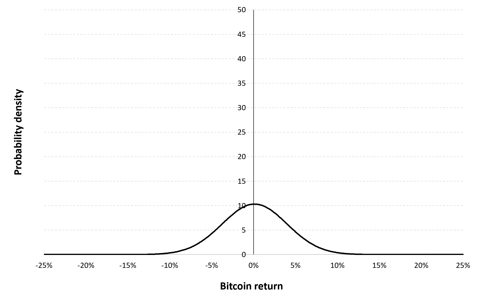
Gaussian distribution

The Gaussian distribution (also called the normal distribution) is a parametric distribution with two parameters: the mean and the standard deviation of returns. We estimated these two parameters over the period from September 17, 2014 to December 31, 2022. The annualized mean of daily returns is equal to 30.81% and the annualized standard deviation of daily returns is equal to 62.33%.

Figure 9 below represents the Gaussian distribution of the Bitcoin daily returns with parameters estimated over the period from September 17, 2014 to December 31, 2022.

Figure 9. Gaussian distribution of the Bitcoin returns.
Gaussian distribution of the daily Bitcoin returns
Source: computation by the author (data: Yahoo! Finance website).

Risk measures of the Bitcoin returns

The R program that you can download above also allows you to compute risk measures about the returns of the Bitcoin.

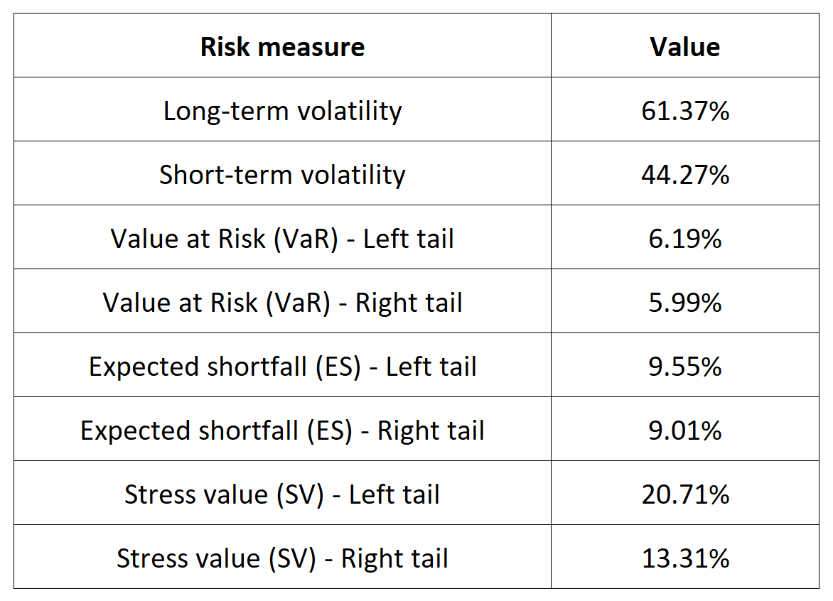
Table 5 below presents the following risk measures estimated for the Bitcoin:

The long-term volatility (the unconditional standard deviation estimated over the entire period)
The short-term volatility (the standard deviation estimated over the last three months)
The Value at Risk (VaR) for the left tail (the 5% quantile of the historical distribution)
The Value at Risk (VaR) for the right tail (the 95% quantile of the historical distribution)
The Expected Shortfall (ES) for the left tail (the average loss over the 5% quantile of the historical distribution)
The Expected Shortfall (ES) for the right tail (the average loss over the 95% quantile of the historical distribution)
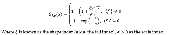
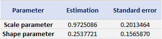
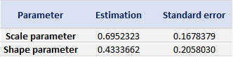
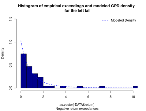
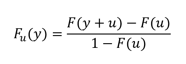
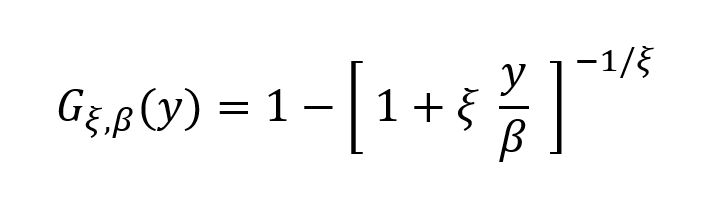
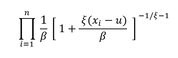
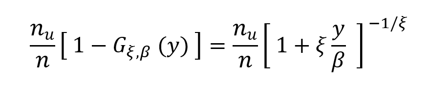
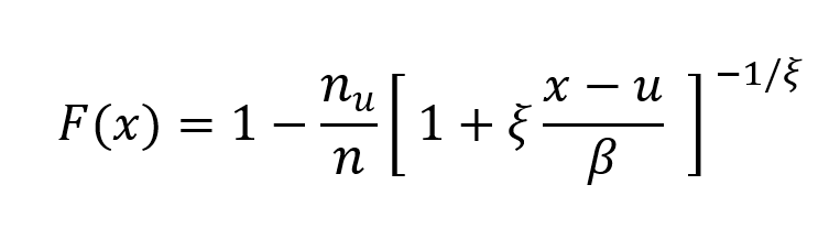
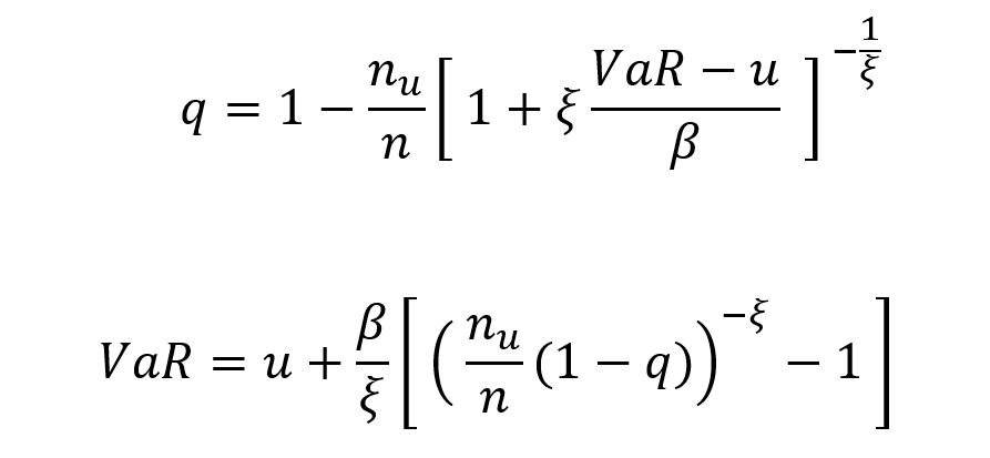
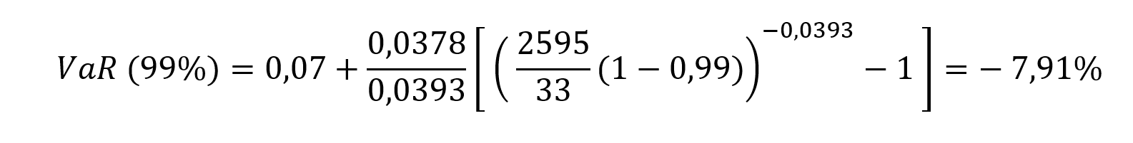
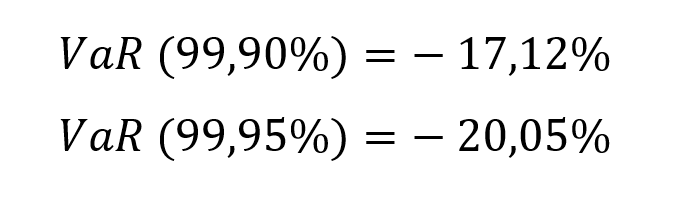
The Stress Value (SV) for the left tail (the 1% quantile of the tail distribution estimated with a Generalized Pareto distribution)
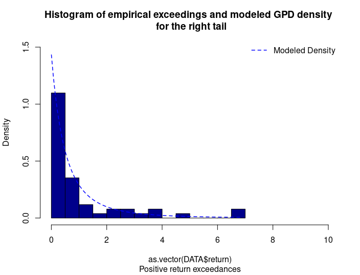
The Stress Value (SV) for the right tail (the 99% quantile of the tail distribution estimated with a Generalized Pareto distribution)

Table 5. Risk measures for the Bitcoin.

Source: computation by the author (data: Yahoo! Finance website).

The volatility is a global measure of risk as it considers all the returns. The Value at Risk (VaR), Expected Shortfall (ES) and Stress Value (SV) are local measures of risk as they focus on the tails of the distribution. The study of the left tail is relevant for an investor holding a long position in the Bitcoin while the study of the right tail is relevant for an investor holding a short position in the Bitcoin.

Why should I be interested in this post?

Students would be keenly interested in this article discussing Bitcoin’s history and trends due to its profound influence on the financial landscape. Bitcoin, as a novel and dynamic asset class, presents a unique opportunity for students to explore the evolving world of finance. By delving into Bitcoin’s past, understanding its market trends, and assessing its impact on global economies, students can equip themselves with the knowledge and skills needed to navigate a financial landscape that is increasingly intertwined with cryptocurrencies and blockchain technology. Moreover, this knowledge can enhance their career prospects in an industry undergoing significant transformation and innovation.

Useful resources

Academic research about risk

Longin F. (2000) From VaR to stress testing: the extreme value approach Journal of Banking and Finance, N°24, pp 1097-1130.

Longin F. (2016) Extreme events in finance: a handbook of extreme value theory and its applications Wiley Editions.

Data

Yahoo! Finance

Yahoo! Finance Historical data for Bitcoin

CoinMarketCap Historical data for Bitcoin

About the author

The article was written in September 2023 by Snehasish CHINARA (ESSEC Business School, Grande Ecole Program – Master in Management, 2022-2024).

Extreme returns and tail modelling of the S&P 500 index for the US equity market

October 20, 2023 by Shengyu ZHENG

Extreme returns and tail modelling of the S&P 500 index for the US equity market

In this article, Shengyu ZHENG (ESSEC Business School, Grande Ecole Program – Master in Management, 2020-2024) describes the statistical behavior of extreme returns of the S&P 500 index for the US equity market and explains how extreme value theory can be used to model the tails of its distribution.

The S&P 500 index for the US equity market

The S&P 500, or the Standard & Poor’s 500, is a renowned stock market index encompassing 500 of the largest publicly traded companies in the United States. These companies are selected based on factors like market capitalization and sector representation, making the index a diversified and reliable reflection of the U.S. stock market. It is a market capitalization-weighted index, where companies with larger market capitalization represent a greater influence on their performance. The S&P 500 is widely used as a benchmark to assess the health and trends of the U.S. economy and as a performance reference for individual stocks and investment products, including exchange-traded funds (ETF) and index funds. Its historical significance, economic indicator status, and global impact contribute to its status as a critical barometer of market conditions and overall economic health.

Characterized by its diversification and broad sector representation, the S&P 500 remains an essential tool for investors, policymakers, and economists to analyze market dynamics. This index’s performance, affected by economic data, geopolitical events, corporate earnings, and market sentiment, can provide valuable insights into the state of the U.S. stock market and the broader economy. Its rebalancing ensures that it remains current and representative of the ever-evolving landscape of American corporations. Overall, the S&P 500 plays a central role in shaping investment decisions and assessing the performance of the U.S. economy.

In this article, we focus on the S&P 500 index of the timeframe from April 1st, 2015, to April 1st, 2023. Here we have a line chart depicting the evolution of the index level of this period. We can observe the overall increase with remarkable drops during the covid crisis (2020) and the Russian invasion in Ukraine (2022).

Figure 1 below gives the evolution of the S&P 500 index from April 1, 2015 to April 1, 2023 on a daily basis.

Figure 1. Evolution of the S&P 500 index.

Source: computation by the author (data: Yahoo! Finance website).

Figure 2 below gives the evolution of the daily logarithmic returns of S&P 500 index from April 1, 2015 to April 1, 2023 on a daily basis. We observe concentration of volatility reflecting large price fluctuations in both directions (up and down movements). This alternation of periods of low and high volatility is well modeled by ARCH models.

Figure 2. Evolution of the S&P 500 index logarithmic returns.

Source: computation by the author (data: Yahoo! Finance website).

Summary statistics for the S&P 500 index

Table 1 below presents the summary statistics estimated for the S&P 500 index:

Table 1. Summary statistics for the S&P 500 index.
summary statistics of the S&P 500 index returns
Source: computation by the author (data: Yahoo! Finance website).

The mean, the standard deviation / variance, the skewness, and the kurtosis refer to the first, second, third and fourth moments of statistical distribution of returns respectively. We can conclude that during this timeframe, the S&P 500 index takes on a slight upward trend, with relatively important daily deviation, negative skewness and excess of kurtosis.

Tables 2 and 3 below present the top 10 negative daily returns and top 10 positive daily returns for the S&P 500 index over the period from April 1, 2015 to April 1, 2023.

Table 2. Top 10 negative daily returns for the S&P 500 index.
Top 10 negative returns of the S&P 500 index
Source: computation by the author (data: Yahoo! Finance website).

Table 3. Top 10 positive daily returns for the S&P 500 index.
Top 10 positive returns of the S&P 500 index
Source: computation by the author (data: Yahoo! Finance website).

Modelling of the tails

Here the tail modelling is conducted based on the Peak-over-Threshold (POT) approach which corresponds to a Generalized Pareto Distribution (GPD). Let’s recall the theoretical background of this approach.

The POT approach takes into account all data entries above a designated high threshold u. The threshold exceedances could be fitted into a generalized Pareto distribution:

Illustration of the POT approach

An important issue for the POT-GPD approach is the threshold selection. An optimal threshold level can be derived by calibrating the tradeoff between bias and inefficiency. There exist several approaches to address this problematic, including a Monte Carlo simulation method inspired by the work of Jansen and de Vries (1991). In this article, to fit the GPD, we use the 2.5% quantile for the modelling of the negative tail and the 97.5% quantile for that of the positive tail.

Based on the POT-GPD approach with a fixed threshold selection, we arrive at the following modelling results for the GPD for negative extreme returns (Table 4) and positive extreme returns (Table 5) for the S&P 500 index:

Table 4. Estimate of the parameters of the GPD for negative daily returns for the S&P 500 index.

Source: computation by the author (data: Yahoo! Finance website).

Table 5. Estimate of the parameters of the GPD for positive daily returns for the S&P 500 index.

Source: computation by the author (data: Yahoo! Finance website).

Figure 3. GPD for the left tail of the S&P 500 index returns.

Source: computation by the author (data: Yahoo! Finance website).

Figure 4. GPD for the right tail of the S&P 500 index returns.

Source: computation by the author (data: Yahoo! Finance website).

Applications in risk management

Extreme Value Theory (EVT) as a statistical approach is used to analyze the tails of a distribution, focusing on extreme events or rare occurrences. EVT can be applied to various risk management techniques, including Value at Risk (VaR), Expected Shortfall (ES), and stress testing, to provide a more comprehensive understanding of extreme risks in financial markets.

Why should I be interested in this post?

Extreme Value Theory is a useful tool to model the tails of the evolution of a financial instrument. In the ever-evolving landscape of financial markets, being able to grasp the concept of EVT presents a unique edge to students who aspire to become an investment or risk manager. It not only provides a deeper insight into the dynamics of equity markets but also equips them with a practical skill set essential for risk analysis. By exploring how EVT refines risk measures like Value at Risk (VaR) and Expected Shortfall (ES) and its role in stress testing, students gain a valuable perspective on how financial institutions navigate during extreme events. In a world where financial crises and market volatility are recurrent, this post opens the door to a powerful analytical framework that contributes to informed decisions and financial stability.

Download R file to model extreme behavior of the index

You can find below an R file (file with txt format) to study extreme returns and model the distribution tails for the S&P 500 index.

Useful resources

Academic resources

Embrechts P., C. Klüppelberg and T. Mikosch (1997) Modelling Extremal Events for Insurance and Finance Springer-Verlag.

Embrechts P., R. Frey, McNeil A.J. (2022) Quantitative Risk Management Princeton University Press.

Gumbel, E. J. (1958) Statistics of extremes New York: Columbia University Press.

Longin F. (2016) Extreme events in finance: a handbook of extreme value theory and its applications Wiley Editions.

Other resources

Extreme Events in Finance

Chan S. Statistical tools for extreme value analysis

Rieder H. E. (2014) Extreme Value Theory: A primer (slides).

About the author

The article was written in October 2023 by Shengyu ZHENG (ESSEC Business School, Grande Ecole Program – Master in Management, 2020-2024).

Les distributions statistiques

October 16, 2023 by Shengyu ZHENG

Distributions statistiques : variable discrète vs variable continue

Dans cet article, Shengyu ZHENG (ESSEC Business School, Grande Ecole – Master in Management, 2020-2024) explique les distributions statistiques pour des variables aléatoires discrètes et continues.

Variables aléatoires discrète et continue

Une variable aléatoire est une variable dont la valeur est déterminée d’après la réalisation d’un événement aléatoire. Plus précisément, la variable (X) est une fonction mesurable depuis un ensemble de résultats (Ω) à un espace mesurable (E).

X : Ω → E

On distingue principalement deux types de variables aléatoires : discrètes et continues.

Une variable aléatoire discrète prend des valeurs dans un ensemble dénombrable comme l’ensemble des entiers naturels. Par exemple, le nombre de points marqués lors d’un match de basket est une variable aléatoire discrète, car elle ne peut prendre que des valeurs entières telles que 0, 1, 2, 3, etc. Les probabilités associées à chaque valeur possible de la variable aléatoire discrète sont appelées probabilités de masse.

En revanche, une variable aléatoire continue prend des valeurs dans un ensemble non dénombrable comme l’ensemble des nombres réels. Par exemple, la taille ou le poids d’une personne sont des variables aléatoires continues, car elles peuvent prendre n’importe quelle valeur réelle positive. Les probabilités associées à une variable aléatoire continue sont déterminées par une fonction de densité de probabilité. Cette fonction permet de mesurer la probabilité que la variable aléatoire se situe dans un intervalle donné de valeurs.

Méthodes pour décrire des distributions statistiques

Afin de mieux comprendre une variable aléatoire, il y a plusieurs moyens pour décrire la distribution de la variable.

Calcul des statistiques

Une statistique est le résultat d’une suite d’opérations appliquées à un ensemble d’observations appelé échantillon et une mesure numérique qui résume une caractéristique de cet ensemble. Par exemple, la moyenne est un exemple de statistiques.
Les statistiques peuvent être divisées en deux types principaux : les statistiques descriptives et les statistiques inférentielles.

Les statistiques descriptives sont utilisées pour résumer et décrire les caractéristiques de base d’un ensemble de données. Elles comprennent des mesures telles que les moments d’une distribution (la moyenne, la variance, le skewness, le kurtosis, …). Une explication plus détaillée est disponible dans l’article Moments de la distribution.

Les statistiques inférentielles, quant à elles, sont utilisées pour faire des inférences sur une population à partir d’un échantillon de données. Elles incluent des tests d’hypothèses, des intervalles de confiance, des analyses de régression, des modèles prédictifs, etc.

Histogramme

Un histogramme est un type de graphique qui permet de représenter la distribution des données d’un échantillon. Il est constitué d’une série de rectangles verticaux, où chaque rectangle représente une plage de valeurs de la variable étudiée (appelée classe), et dont la hauteur correspond à la fréquence des observations de cette classe.

L’histogramme est un outil très utilisé pour visualiser la distribution des données et pour identifier les tendances et les formes dans les données pour les variables discrètes ainsi que continues discrétisées.

Fonction de masse et fonction de densité

Une fonction de masse de probabilité est une fonction mathématique qui permet de décrire la distribution de probabilité d’une variable aléatoire discrète.

La fonction de masse de probabilité associe à chaque valeur possible de la variable aléatoire discrète une probabilité. Par exemple, si X est une variable aléatoire discrète prenant les valeurs 1, 2, 3 et 4 avec des probabilités respectives de 0,2, 0,3, 0,4 et 0,1, alors la fonction de masse de probabilité de X (loi multinomiale) est donnée par :
P(X=1) = 0,2
P(X=2) = 0,3
P(X=3) = 0,4
P(X=4) = 0,1

Il est important de noter que la somme des probabilités pour toutes les valeurs possibles de la variable aléatoire doit être égale à 1, c’est-à-dire, pour toute variable aléatoire discrète X :
∑ P(X=x) = 1

Figure 1. Fonction de masse d’une loi multinomiale (pour une variable discrète).

Source : calcul par l’auteur

Par contre, une fonction de densité représente la distribution de probabilité d’une variable aléatoire continue. La fonction de densité permet de calculer la probabilité que la variable aléatoire prenne une valeur dans un intervalle donné.
Graphiquement, l’aire sous la courbe de la fonction de densité entre deux valeurs a et b correspond à la probabilité que la variable aléatoire prenne une valeur dans l’intervalle [a, b].

Il est important de noter que la fonction de densité est une fonction continue, positive et intégrable sur tout son domaine. L’intégrale de la fonction de densité sur l’ensemble des valeurs possibles de la variable aléatoire est égale à 1.

Figure 2. Fonction de densité d’une loi normale (pour une variable continue).

Source : calcul par l’auteur

Fonction de répartition

La fonction de répartition (ou fonction de distribution cumulative) est une fonction mathématique qui décrit la probabilité qu’une variable aléatoire prenne une valeur inférieure ou égale à une certaine valeur donnée. Elle est définie pour toutes les variables aléatoires, qu’elles soient continues ou discrètes.
Pour une variable aléatoire discrète, la fonction de répartition F(x) est définie comme la somme des probabilités des valeurs inférieures ou égales à x :

F(x) = P(X ≤ x) = Σ P(X = xi) pour xi ≤ x

Pour une variable aléatoire continue, la fonction de répartition F(x) est définie comme l’intégrale de la densité de probabilité f(x) de -∞ à x :
F(x)=P(X≤x)= ∫_-∞^xf(t)dt

Exemples

Dans cette partie, nous allons prendre deux exemples d’analyse de distribution statistique, l’un d’une variable aléatoire discrète et l’autre d’une variable continue.

Variable discrète : résultat du lancer d’un dé à six faces

Le jeu de lancer de dé à six faces consiste à lancer un dé pour obtenir un résultat aléatoire entre 1 et 6, correspondant aux six faces du dé. Les résultats ne prennent que les valeurs entières (1, 2, 3, 4, 5 et 6) et ils ont tous une probabilité identique de 1/6.

Dans cet exemple, le code R permet de simuler N lancers de dé et de visualiser la distribution des N résultats à l’aide d’un histogramme. En utilisant ce code, il est possible de simuler des parties de lancer de dé et d’analyser les résultats pour mieux comprendre la distribution des probabilités.

Si cette expérience aléatoire est répétée 1 000 fois, nous arrivons à un résultat dont l’histogramme est comme :

Figure 3. Histogramme des résultats de lancers d’un dé à six faces.

Source : calcul par l’auteur

Nous constatons que les résultats sont distribués d’une manière équilibrée et ont la tendance de converger vers la probabilité théorique 1/6.

Variable continue : rendments de l’indice CAC40

Le rendement d’un indice d’actions comme le CAC 40 pour le marché français est une variable aléatoire continue parce qu’elle peut prendre toutes les valeurs réelles.

Nous utilisons un historique de l’indice boursier journalier pour des cours de clôture de l’indice CAC 40 du 1^er avril 2021 au 1^er avril 2023 pour calculer des rendements journalières (rendements logarithmiques).

En finance, la distribution des rendements journalières de l’indice CAC 40 est souvent modélisée par une loi normale, même si la loi normale ne modélise pas forcément bien la distribution observée, surtout les queues de distributions observées. Dans le graphique ci-dessous, nous voyons que la distribution normale ne décrit pas bien la distribution réelle.

Figure 4. Fonction de densité des rendements journalières de l’indice CAC 40 (variable continue).

Source : calcul par l’auteur

Pour des observations issues pour une variable continue, il est toujours possible de regrouper les observations dans des intervalles et de représenter dans un histogramme.

La table 1 ci-dessous donne les statistiques descriptives pour les rendements journalières de l’indice CAC 40.

Table 1. Statistiques descriptives pour les rendements journalières de l’indice CAC 40.

Statistiques descriptives	Valeur
Moyenne	0.035
Médiane	0.116
Écart-type	1.200
Skewness	-0.137
Kurtosis	6.557

Les résultats du calcul des statistiques descriptives correspondent bien à ce que nous pouvons remarquer du graphique. La distribution des rendements a une moyenne légèrement positive. La queue de la distribution empirique est plus épaisse que celle de la distribution normale vu les survenances des rendements (positives ou négatives) extrêmes.

Fichier R pour cet article

A propos de l’auteur

Cet article a été écrit en octobre 2023 par Shengyu ZHENG (ESSEC Business School, Grande Ecole Program – Master in Management, 2020-2024).

My experience as Actuarial Apprentice at La Mutuelle Générale

October 9, 2023 by Shengyu ZHENG

My experience as Actuarial Apprentice at La Mutuelle Générale

In this article, Shengyu ZHENG (ESSEC Business School, Grande Ecole Program – Master in Management, 2020-2024) shares his professional experience as Actuarial Apprentice at La Mutuelle Générale .

About the company

La Mutuelle Générale is a major French mutual insurance company that has established itself as a trusted provider of health and social protection solutions. With a history dating back to its foundation in 1945 as the mutual health insurance provider for La Poste et France Télécom, La Mutuelle Générale has grown to become a key player in the mutual health insurance sector in France.

Unlike private insurance companies, mutual insurance companies are based on the concept of solidarity and not for lucrative purposes. As a mutual insurance company, La Mutuelle Générale has no shareholders but only member clients who also contribute to the decision making of the company.

Specializing in health insurance and complementary health coverage, La Mutuelle Générale offers a comprehensive range of insurance products and services designed to meet the diverse needs of both individual and collective clients. On top of the coverage offered by the French social security system, la Mutuelle Générale’s health insurance offerings encompass a wide array of guarantees, including medication reimbursement, hospitalization coverage, dental care, optical care, and so forth. The company strives to provide flexible and tailored solutions to suit the specific requirements of the member clients.

The core business of the mutual insurance company is composed of health insurance and social protection (short-term incapacity, long-term invalidity, dependency and death). For the purpose of providing a more comprehensive healthcare service, in 2020, the company launched its Flex service platform, which enables partner companies to access services such as home care or personal assistance.

Overall, La Mutuelle Générale stands as a reliable and reputable insurance company, driven by the mission to provide quality healthcare coverage and social protection to individuals and businesses across France. They combine their extensive expertise, expansive coverage, and a dedicated workforce to promote well-being, financial security in face of healthcare needs, and peace of mind for their members.

Logo of La Mutuelle Générale

Source: website of La Mutuelle Générale

My position

Since September 2022, I have been engaged in a one-year apprenticeship contract for the position of Actuarial Analyst in the Technical Department that englobes all the actuarial missions. Specifically, I was in the team of Studies and Products Collective Health Insurance and Social Protection. This team takes charge of the actuarial studies of social protections and collective health insurance contracts.

My missions

Within the team, I had the chance to assist my colleagues to conduct actuarial studies in various subjects:

Monitor the profitability and risk of different insurance portfolios

We continually evaluate the financial performance and risk exposure associated with individual and group Health Insurance and Life Insurance policies. We assess factors such as claims experience, investment returns, and expenses to gauge the profitability and financial health of the portfolios. By closely monitoring these aspects, the management can make informed decisions to ensure the sustainability and growth of the company.

Calculate and provide rates for group Health Insurance and Life Insurance products

We are responsible for developing the pricing structure and tools for group Health Insurance and Life Insurance products. According to the size of the clients, we deploy different pricing strategies.

We model factors such as the demographics and health profiles of the insured individuals, expected claims frequency and severity, and desired profit margins. Through mathematical models and statistical analysis, we determine appropriate premia for corresponding products.

Here I introduce brief the key idea of insurance pricing. The mechanism of insurance is that the insured person pays for a premium beforehand to get guarantee against a certain risk for a period in the future. Insurance works on the basis of mutualisation, explained by the Law of Large Numbers. For example, for automobile insurance against the risk of theft. The risk does not befall everyone (the probability of occurrence is relatively low). Whereas, when it happens, the owner has to endure a loss amount that is relatively high and it is in this case that insurance companies accompany the car owner to cover part or all of the loss if the owner is insured.

Let’s denote X_i as the loss amount for insured person i (X_i equals 0 if the risk does not take place). If an insurance company has n insured persons, and we assume all X_i are independent and identically distributed. According to the Law of Large Numbers, we have:

1/n ∑ ⁿ_{i =1} X_i → 𝔼[ X_i]

If n is large enough, the total claim amount will converge to 𝔼[ X₁]. Therefore, if every insured person pays individually a premium of 𝔼[ X₁], the insurance company as a whole would be able to pay off all the possible claims.

Ensure the implementation of the underwriting policy:

The Underwriting Department relies on a tool to assess and price group insurance contracts. Actuaries play a crucial role in guaranteeing the consistency and accuracy of the pricing scales used within this tool. We review and validate the formulas and algorithms used to calculate premia, to make sure that they are aligned with the company’s underwriting guidelines and principles and with our calculations.

We work closely with the underwriting team to enforce the company’s underwriting policy. This involves establishing guidelines and criteria for accepting or rejecting insurance applications, determining coverage limits, and setting appropriate pricing. We provide insights and recommendations based on their analyses to ensure the underwriting policy is effectively implemented, balancing risk management and business objectives.

Conduct studies related to the current political and economic conditions

Given the dynamic nature of the insurance sector, we conduct studies to assess the impact of external factors, such as economic conditions, on insurance products. For example, we analyze the effects of the 100% Santé reform on insurance premia and claim payouts. We also conduct theoretical research of the impact of the 2023 retirement reform on our social protection portfolio.

By understanding these impacts, actuaries can adapt pricing strategies, adjust risk models, and make informed decisions to address emerging challenges and provide appropriate coverage to policyholders in conformity with the framework of regulations.

Required skills and knowledge

First and foremost, the position pivoted on actuarial studies requires solid understanding of actuarial and insurance concepts and theories. For example, it is indispensable to understand the contractual aspects of insurance policies, pricing theories and accounting rules of insurance products. Actuary is a profession that requires high-level specified expertise, and the title of Actuary is recognized by actuarial associations in respective countries after passing the credentialing process.

Besides, statistical and information techniques are highly needed. The professions of Actuary could be in a way considered as a combination of Statistician, Informatician and Marketer. Making use of statistical and information techniques, actuaries delve deep into data to uncover useful information that would aid the pricing of insurance policies and the decision-making process.

Last but not least, since the insurance sector is highly regulated and insurance offerings are mostly homogeneous, a solid and comprehensive knowledge of the local regulatory environment and business landscape is a must to make sure efficient development and management of the product portfolio. In my case, a thorough understanding of the French social security system and product specificities is crucial.

What I have learned

This apprenticeship experience takes place in parallel with my double curriculum in Actuarial Science at Institut de Statistique de Sorbonne Université (ISUP). I had the opportunities to apply the theoretical aspects in actual projects and work on various subjects with the guidance of experienced professionals. I had the chance to deepen my understanding in insurance pricing, health insurance & social protection and risk management for insurers.

Financial concepts related my internship

Insurance pricing

Health insurance pricing involves the application of theoretical concepts and statistical analysis to assess risk, project future claims, and determine suitable premiums. Insurers utilize statistical models to evaluate factors such as age, gender, pre-existing conditions, and healthcare utilization patterns to estimate the likelihood and cost of potential claims. By considering risk pooling, loss ratios, and health economic studies, insurers strive to set premiums that balance financial sustainability while providing adequate coverage to policyholders. Regulatory guidelines and statistical modeling further contribute to the development of pricing strategies in health insurance.

Solvency II

Solvency II is a regulatory framework for insurance companies in the European Union (EU) that aims to ensure financial stability and solvency. It establishes risk-based capital requirements, governance standards, and disclosure obligations for insurers. Under Solvency II, insurers are required to assess and manage their risks, maintain sufficient capital to withstand potential losses, and regularly report their financial and risk positions to regulatory authorities. The framework promotes a comprehensive approach to risk management, aligning capital requirements with the underlying risks of insurance activities and enhancing transparency and accountability in the insurance sector.

Useful resources

La Mutuelle Générale

Institut des Actuaires

Pricing Insurance #1: Pure Premium Method

About the author

The article was written in October 2023 by Shengyu ZHENG (ESSEC Business School, Grande Ecole Program – Master in Management, 2020-2024).

Application de la théorie des valeurs extrêmes en finance de marchés

February 4, 2024October 6, 2023 by Gabriel FILJA

Dans cet article, Gabriel FILJA (ESSEC Business School, Executive Master in Senior Bank Management, 2022-2023 & Head of Hedging à Convera) présente des applications de la théorie des valeurs extrêmes en finance de marchés et notamment en gestion des risques de marchés.

Principe

La théorie des valeurs extrêmes (TVE), appelé théorème de Fisher-Tippet-Gnedenko tente de fournir une caractérisation complète du comportement de la queue pour tous les types de distributions de probabilités.

La théorie des valeurs extrêmes montre que la loi asymptotique des rentabilités minimale et maximale a une forme bien déterminée qui est largement indépendante du processus de rentabilités lui-même (le lien entre les deux distributions apparaît en particulier dans la valeur de l’indice de queue qui reflète le poids des queues de distribution). L’intérêt de la TVE dans la gestion du risque c’est de pouvoir calculer le quantile au-delà de 99% du seuil de confiance dans le cadre des stress tests ou de la publication des exigences réglementaires.

Gnedenko a démontré en 1943 par la Théorie des valeurs extrêmes la propriété qui s’applique à des nombreuses distributions de probabilités. Soit F(x) la fonction de répartition d’une variable x. u est une valeur de x située dans la partie droite de la queue de distribution.

La probabilité que x soit compris entre u et u+y est de F(y+u) – F(u) et la probabilité que x soit supérieur à u est 1-F(u). Soit F_u(y) la probabilité conditionnelle que x soit compris entre u et u+y sachant que x>u∶

Probabilité conditionnelle

Estimation des paramètres

Selon les résultats de Gnedenko, pour un grand nombre de distribution, cela converge vers une distribution généralisée de Pareto au fur et à mesure que u augmente :

Distribution_généralisée_Pareto

β est le paramètre d’échelle représente la dispersion de la loi des extrêmes
ξ est l’indice de queue qui mesure l’épaisseur de la queue et la forme

Selon la valeur de l’indice de queue, on distingue trois formes dedistribiution d’extrêmes :

Frechet ξ > 0
Weibull ξ < 0
Gumbel ξ = 0

L’indice de queue ξ reflète le poids des extrêmes dans la distribution des rentabilités. Une valeur positive de l’indice de queue signifie que les extrêmes n’ont pas de rôle important puisque la variable est bornée. Une valeur nulle donne relativement peu d’extrêmes alors qu’une valeur négative implique un grand nombre d’extrêmes (c’est le cas de la loi normale).

Figure 1 : Densité des lois des valeurs extrêmes

Source : auteur.

Tableau 1 : Fonctions de distribution des valeurs extrêmes pour un ξ > 0, loi de Frechet, ξ < 0 loi de Weibull et ξ = 0, loi de Gumbel.
Source : auteur.

Les paramètres β et ξ sont estimés par la méthode de maximum de vraisemblance. D’abord il faut définir u (valeur proche du 95e centile par exemple). Une des méthodes pour déterminer ce seuil, c’est la technique appelée Peak Over Threshold (POT), ou méthode des excès au-delà d’un seuil qui se focalise sur les observations qui dépassent un certain seuil donné. Au lieu de considérer les valeurs maximales ou les plus grandes valeurs, cette méthode consiste à examiner toutes les observations qui franchissent un seuil élevé préalablement fixé.
L’objectif est de sélectionner un seuil adéquat et d’analyser les excès qui en découlent. Ensuite nous trions les résultats par ordre décroissant pour obtenir les observations telles que x>u et leur nombre total.

Nous étudions maintenant les rentabilités extrêmes pour l’action Société Générale sur la période 2011-2021. La Figure 2 représentes rentabilités journalières de l’action et les rentabilités extrêmes négatives obtenues avec l’approche des dépassements de seuil (Peak Over Threshold ou POT). Avec le seuil retenu de -7%, on obtient 33 dépassements sur 2 595 rentabilités journalières de la période 2011 à 2021.

Figure 2 : Sélection des rentabilités extrêmes négatives pour l’action Société Générale selon l’approche Peak Over Threshold (POT)

Source : auteur.

Méthode d’estimation statistique

Nous allons maintenant voir comment déterminer les β et ξ en utilisant la fonction de maximum de vraisemblance qui s’écrit :

Fonction de vraisemblance

Pour un échantillon de n observations, l’estimation de 1-F(u) est n_u/n. Dans ce cas, la probabilité inconditionnelle de x>u+y vaut :

Fonction de vraisemblance

Et l’estimateur de la queue de distribution de probabilité cumulée de x (pour un grand) est :

Estimateur queue distribution

Mon travail personnel a consisté à estimer le paramètre d’échelle β et le paramètre de queue ξ à partir de la formule par le maximum de vraisemblance en utilisant le solveur Excel. Nous avons précédemment déterminé n=0,07 par la méthode de POT en Figure 2, et n_u= 2595

Ainsi nous obtenons β=0,0378 et ξ=0,0393 ce qui maximise par la méthode du maximum de vraisemblance la somme du logarithme des valeurs extrêmes à un total de 73,77.

Estimation de la VaR TVE

Pour calculer le VaR au seuil q, nous obtenons F(VaR) = q

VaR TVE

Mon travail personnel a consisté à estimer la VaR du titre de la Société Générale de la période de 2011 à 2021 sur un total de 2595 cotations avec 33 dépassements de seuil (-7%). En appliquant les données obtenues à la formule nous obtenons :

VaR 99% Société Générale

Puis nous estimons la VaR à 99,90% et 99,95% :

VaR 99,90% Société Générale

Il n’est pas surprenant que l’extrapolation à la queue d’une distribution de probabilité soit difficile, pas parce qu’il est difficile d’identifier des distributions de probabilité possibles qui pourraient correspondre aux données observées (il est relativement facile de trouver de nombreuses distributions possibles différentes), mais parce que l’éventail des réponses qui peuvent vraisemblablement être obtenues peut être très large, en particulier si nous voulons extrapoler dans la queue lointaine où il peut y avoir peu ou pas de points d’observation directement applicables.

La théorie des valeurs extrêmes, si elle est utilisée pour modéliser le comportement de la queue au-delà de la portée de l’ensemble de données observées, est une forme d’extrapolation. Une partie de la cause du comportement à queue épaisse (fat tail) est l’impact que le comportement humain (y compris le sentiment des investisseurs) a sur le comportement du marché.

En quoi ça peut m’intéresser ?

Nous pouvons ainsi mener des stress tests en utilisant la théorie des valeurs extrêmes et évaluer les impacts sur le bilan de la banque ou encore déterminer les limites de risques pour le trading et obtenir ainsi une meilleure estimation du worst case scenario.

Autres articles sur le blog SimTrade

▶ Shengyu ZHENG Catégories de mesures de risques

▶ Shengyu ZHENG Moments de la distribution

▶ Shengyu ZHENG Extreme Value Theory: the Block-Maxima approach and the Peak-Over-Threshold approach

Ressources

Articles académiques

Falk M., J. Hüsler, et R.-D. Reiss, Laws of Small Numbers: Extremes and Rare Events. Basel: Springer Basel, 2011. doi: 10.1007/978-3-0348-0009-9.

Gilli M. et E. Këllezi, « An Application of Extreme Value Theory for Measuring Financial Risk », Comput Econ, vol. 27, no 2, p. 207‑228, mai 2006, doi: 10.1007/s10614-006-9025-7.

Gkillas K. and F. Longin (2018) Financial market activity under capital controls: lessons from extreme events Economics Letters, 171, 10-13.

Gnedenko B., « Sur La Distribution Limite Du Terme Maximum D’Une Serie Aleatoire », Annals of Mathematics, vol. 44, no 3, p. 423‑453, 1943, doi: 10.2307/1968974.

Hull J.et A. White, « Optimal delta hedging for options », Journal of Banking & Finance, vol. 82, p. 180‑190, sept. 2017, doi: 10.1016/j.jbankfin.2017.05.006.

Longin F. (1996) The asymptotic distribution of extreme stock market returns Journal of Business, 63, 383-408.

Longin F. (2000) From VaR to stress testing : the extreme value approach Journal of Banking and Finance, 24, 1097-1130.

Longin F. (2016) Extreme events in finance: a handbook of extreme value theory and its applications Wiley Editions.

Longin F. and B. Solnik (2001) Extreme Correlation of International Equity Markets, The Journal of Finance, 56, 649-676.

Roncalli T. et G. Riboulet, « Stress testing et théorie des valeurs extrêmes : une vision quantitée du risque extrême ».

Sites internet

Extreme Events in Finance

A propos de l’auteur

Cet article a été écrit en juillet 2023 par Gabriel FILJA (ESSEC Business School, Executive Master in Senior Bank Management, 2022-2023 & Head of Hedging à Convera).

How to get crypto data

March 25, 2024October 4, 2023 by Snehasish CHINARA

How to get crypto data

In this article, Snehasish CHINARA (ESSEC Business School, Grande Ecole Program – Master in Management, 2022-2024) explains how to get crypto data.

Types of data

Number of coins

The information on the number of coins in circulation for a given currency is important to compute its market capitalization. Market capitalization is calculated by multiplying the current price of the cryptocurrency by its circulating number of coins (supply). This metric gives a rough estimate of the cryptocurrency’s total value within the market and its relative size compared to other cryptocurrencies. A lower circulating supply often implies a greater level of scarcity and rarity.

For cryptocurrencies (unlike fiat money), the number of coins in circulation is given by a mathematical formula. The number of coins may be limited (like the Bitcoin) or unlimited (like Ethereum and Dogecoin) over time.

Cryptocurrencies with limited supplies, such as Bitcoin’s maximum supply of 21 million coins, can be perceived as more valuable due to their finite nature. Scarcity can contribute to investor interest and potential price appreciation over time. A lower circulating supply might indicate the potential for future adoption and value appreciation, as the limited supply can create scarcity-driven demand, especially if the cryptocurrency gains more utility and usage.

Bitcoin’s blockchain also relies on a key equation to steadily allow new BTC to be introduced. The equation below gives the total supply of bitcoins:

Total supply of bitcoins

Figure 1 below represents the evolution of the supply of Bitcoins.

Figure 1. Evolution of the supply of Bitcoins

Source: computation by the author.

Market price of a coin

The market price of a cryptocurrency in the market holds crucial insights into how well the cryptocurrency is faring. Although not the sole factor, the market price significantly contributes to evaluating the cryptocurrency’s performance and its prospects. The market price of a cryptocurrency is a dynamic and intricate element that reflects a multitude of factors, both intrinsic and extrinsic. The gradual rise in market value over time indicates a willingness among investors and traders to offer higher prices for the cryptocurrency. This signifies a rising interest and strong belief in the project’s potential for the future. The market price reflects the collective sentiment of investors and traders. Comparing the market price of a cryptocurrency to other similar cryptocurrencies or benchmark assets like Bitcoin can provide insights into its relative strength and performance within the market. A rising market price can indicate increasing adoption of the cryptocurrency for various use cases. Successful projects tend to attract more users and real-world applications, which can drive up the price.

The value of cryptocurrencies in the market is influenced by a variety of elements, with each factor contributing uniquely to their pricing. One of the most significant influences is market sentiment and investor psychology. These factors can cause prices to shift based on positive news, regulatory changes, or reactive selling due to fear. Furthermore, the real-world implementation and usage of a cryptocurrency are crucial for its prosperity. Concrete use cases such as Decentralized Finance (DeFi), Non-Fungible Tokens (NFTs), and international transactions play a vital role in creating demand and propelling price appreciation. Meanwhile, adherence to basic economic principles is evident in the supply-demand dynamics, where scarcity due to limited issuance, halving events, and token burns interact with the balance between supply and demand.

With the number of coins in circulation, the information on the price of coins for a given currency is also important to compute its market capitalization.

Figure 2 below represents the evolution of the price of Bitcoin in US dollar over the period October 2014 – August 2023. The price corresponds to the “closing” price (observed at 10:00 PM CET at the end of the month).

Figure 2. Evolution of the Bitcoin price

Source: computation by the author (data source: Yahoo! Finance).

Trading volume

Trading volume is crucial when assessing the health, reliability, and potential price movements of a cryptocurrency. Trading volume refers to the total amount of a cryptocurrency that is bought and sold within a specific time frame, typically measured in units of the cryptocurrency (e.g., BTC) or in terms of its equivalent value in another currency (e.g., USD).

Trading volume directly mirrors market liquidity, with higher volumes indicative of more liquid markets. This liquidity safeguards against drastic price fluctuations when trading, contrasting with low-volume scenarios that can breed volatility, where even a single substantial trade may disproportionately shift prices. Price alterations are most reliable and meaningful when accompanied by substantial trading volume. Price movements upheld by heightened volume often hold greater validity, potentially pointing to more pronounced market sentiment. When price surges parallel rising trading volume, it suggests a sustainable upward trajectory. Conversely, low trading volume amid rising prices may hint at a forthcoming correction or reversal. Scrutinizing the correlation between price oscillations and trading volume can uncover potential divergences. For instance, ascending prices coupled with dwindling trading volume may suggest a weakening trend.

Figure 3 below represents the evolution of the monthly trading volume of Bitcoin over the period October 2014 – July 2023.

Figure 3. Evolution of the trading volume of Bitcoin

Source: computation by the author (data source: Yahoo! Finance).

Bitcoin data

You can download the Excel file with Bitcoin data used in this post as an illsutration.

Python code

You can download the Python code used to download the data from Yahoo! Finance.

Python script to download Bitcoin historical data and save it to an Excel sheet:

import yfinance as yf
import pandas as pd

# Define the ticker symbol and date range
ticker_symbol = “BTC-USD”
start_date = “2020-01-01”
end_date = “2023-01-01”

# Download historical data using yfinance
data = yf.download(ticker_symbol, start=start_date, end=end_date)

# Create a Pandas DataFrame
df = pd.DataFrame(data)

# Create a Pandas Excel writer object
excel_writer = pd.ExcelWriter(‘bitcoin_historical_data.xlsx’, engine=’openpyxl’)

# Write the DataFrame to an Excel sheet
df.to_excel(excel_writer, sheet_name=’Bitcoin Historical Data’)

# Save the Excel file
excel_writer.save()

print(“Data has been saved to bitcoin_historical_data.xlsx”)

# Make sure you have the required libraries installed and adjust the “start_date” and “end_date” variables to the desired date range for the historical data you want to download.

APIs

Calculating the total number of Bitcoins in circulation over time
Access – Bitcoin Blockchain data
By running a Bitcoin node or by using blockchain data providers like Blockchain.info, Blockchair, or a similar service.

Extract Block Data: Once you have access to the blockchain data, you would need to extract information from each block. Each block contains a record of the transactions that have occurred, including the creation (mining) of new Bitcoins in the form of a “Coinbase” transaction.

Calculate Cumulative Supply: You can calculate the cumulative supply of Bitcoins by adding up the rewards from each block’s Coinbase transaction. Initially, the block reward was 50 Bitcoins, but it halves approximately every four years due to the Bitcoin halving events. So, you’ll need to account for these halving in your calculations.

Code – python

import requests

# Replace ‘YOUR_API_KEY’ with your CoinMarketCap API key
api_key = ‘YOUR_API_KEY’

# Define the endpoint URL for CoinMarketCap’s API
url = ‘https://pro-api.coinmarketcap.com/v1/cryptocurrency/quotes/latest’

# Define the parameters for the request
params = {
‘symbol’: ‘BTC’,
‘convert’: ‘USD’,
‘CMC_PRO_API_KEY’: api_key
}

# Send the request to CoinMarketCap
response = requests.get(url, params=params)

# Parse the response JSON
data = response.json()

# Extract the circulating supply from the response
circulating_supply = data[‘data’][‘BTC’][‘circulating_supply’]

print(f”Current circulating supply of Bitcoin: {circulating_supply} BTC”)

## Replace ‘YOUR_API_KEY’ with your actual CoinMarketCap API key.

Why should I be interested in this post?

Cryptocurrency data is becoming increasingly relevant in these fields, offering opportunities for research, data analysis skill development, and even career prospects. Whether you’re aiming to conduct research, stay informed about the evolving financial landscape, or simply enhance your data analysis abilities, understanding how to access and work with crypto data is an asset. Plus, as the cryptocurrency industry continues to grow, this knowledge can open new career paths and improve your personal finance decision-making. In a rapidly changing world, diversifying your knowledge with cryptocurrency data acquisition skills can be a wise investment in your future.

Useful resources

APIs

CoinMarketCap Source of API keys and program

CoinGecko Source of API keys and Programs

CryptoNews Source of API keys and Programs

Data sources

Yahoo! Finance Historical data for Bitcoin

Coinmarketcap Historical data for Bitcoin

Blockchain.com Market Data and charts on Bitcoin history

About the author

The article was written in October 2023 by Snehasish CHINARA (ESSEC Business School, Grande Ecole Program – Master in Management, (2022-2024).

Bitcoin: the mother of all cryptocurrencies

Historical context and background

Key features and use cases

Technology and underlying blockchain

Supply of coins

Historical data for Bitcoin

How to get the data?

Historical data for the Bitcoin market prices

Python code

R code

Data file

Evolution of the Bitcoin

Summary statistics for the Bitcoin

Statistical distribution of the Bitcoin returns

Historical distribution

Gaussian distribution

Risk measures of the Bitcoin returns

Why should I be interested in this post?

Related posts on the SimTrade blog

About cryptocurrencies

About statistics

Useful resources

Academic research about risk

Data

About the author

Extreme returns and tail modelling of the S&P 500 index for the US equity market

The S&P 500 index for the US equity market

Summary statistics for the S&P 500 index

Modelling of the tails

Applications in risk management

Why should I be interested in this post?

Download R file to model extreme behavior of the index

Related posts on the SimTrade blog

About financial indexes

About portfolio management

About statistics

Useful resources

Academic resources

Other resources

About the author

Distributions statistiques : variable discrète vs variable continue

Variables aléatoires discrète et continue

Méthodes pour décrire des distributions statistiques

Calcul des statistiques

Histogramme

Fonction de masse et fonction de densité

Fonction de répartition

Exemples

Variable discrète : résultat du lancer d’un dé à six faces

Variable continue : rendments de l’indice CAC40

Table 1. Statistiques descriptives pour les rendements journalières de l’indice CAC 40.

Fichier R pour cet article

A propos de l’auteur

My experience as Actuarial Apprentice at La Mutuelle Générale

About the company

My position

My missions

Monitor the profitability and risk of different insurance portfolios

Calculate and provide rates for group Health Insurance and Life Insurance products

Ensure the implementation of the underwriting policy:

Conduct studies related to the current political and economic conditions

Required skills and knowledge

What I have learned

Financial concepts related my internship

Insurance pricing

Solvency II

Related posts on the SimTrade blog

Useful resources

About the author

Principe

Estimation des paramètres

Méthode d’estimation statistique

Estimation de la VaR TVE

En quoi ça peut m’intéresser ?

Autres articles sur le blog SimTrade

Ressources

Articles académiques

Sites internet

A propos de l’auteur

How to get crypto data