

In this article, Jayati WALIA (ESSEC Business School, Grande Ecole – Master in Management, 2019-2022) explains the Monte Carlo simulation method for VaR calculation.
Introduction
Monte Carlo simulations are a broad class of computational algorithms that rely majorly on repeated random sampling to obtain numerical results. The underlying concept is to model the multiple possible outcomes of an uncertain event. It is a technique used to understand the impact of risk and uncertainty in prediction and forecasting models.
The Monte Carlo simulation method was invented by John von Neumann (Hungarian-American mathematician and computer scientist) and Stanislaw Ulam (Polish mathematician) during World War II to improve decision making under uncertain conditions. It is named after the popular gambling destination Monte Carlo, located in Monaco and home to many famous casinos. This is because the random outcomes in the Monte Carlo modeling technique can be compared to games like roulette, dice and slot machines. In his autobiography, ‘Adventures of a Mathematician’, Ulam mentions that the method was named in honor of his uncle, who was a gambler.
Calculating VaR using Monte Carlo simulations
The basic concept behind the Monte Carlo approach is to repeatedly run a large number of simulations of a random process for a variable of interest (such as asset returns in finance) covering a wide range of possible scenarios. These variables are drawn from pre-specified probability distributions that are assumed to be known, including the analytical function and its parameters. Thus, Monte Carlo simulations inherently try to recreate the distribution of the return of a position, from which VaR can be computed.
Consider the CAC40 index as our asset of interest for which we will compute the VaR using Monte Carlo simulations.
The first step in the simulation is choosing a stochastic model for the behavior of our random variable (the return on the CAC 40 index in our case).
A common model is the normal distribution; however, in this case, we can easily compute the VaR from the normal distribution itself. The Monte Carlo simulation approach is more relevant when the stochastic model is more complex or when the asset is more complex, leading to difficulties to compute the VaR. For example, if we assume that returns follow a GARCH process, the (unconditional) VaR has to be computed with the Monte Carlo simulation methods. Similarly, if we consider complex financial products like options, the VaR has to be computed with the Monte Carlo simulation methods.
In this post, we compare the Monte Carlo simulation method with the historical method and the variance-covariance method. Thus, we simulate returns for the CAC40 index using the GARCH (1,1) model.
Figure 1 and 2 illustrate the GARCH simulated daily returns and volatility for the CAC40 index.
Figure 1. Simulated GARCH daily returns for the CAC40 index.
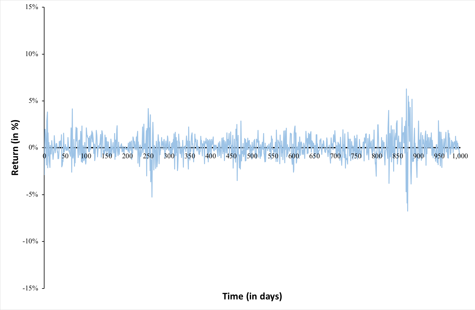
Source: computation by the author.
Figure 2. Simulated GARCH daily volatility for the CAC40 index.
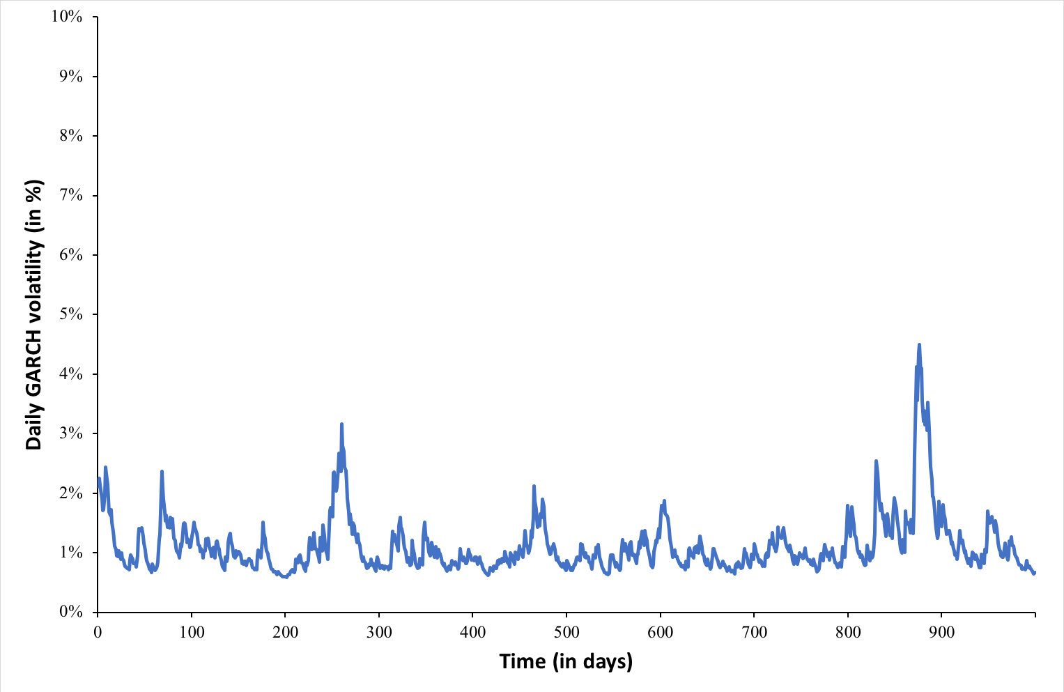
Source: computation by the author.
Next, we sort the distribution of simulated returns in ascending order (basically in order of worst to best returns observed over the period). We can now interpret the VaR for the CAC40 index in one-day time horizon based on a selected confidence level (probability).
For instance, if we select a confidence level of 99%, then our VaR estimate corresponds to the 1st percentile of the probability distribution of daily returns (the bottom 1% of returns). In other words, there are 99% chances that we will not obtain a loss greater than our VaR estimate (for the 99% confidence level). Similarly, VaR for a 95% confidence level corresponds to bottom 5% of the returns.
Figure 3 below represents the unconditional probability distribution of returns for the CAC40 index assuming a GARCH process for the returns.
Figure 3. Probability distribution of returns for the CAC40 index.
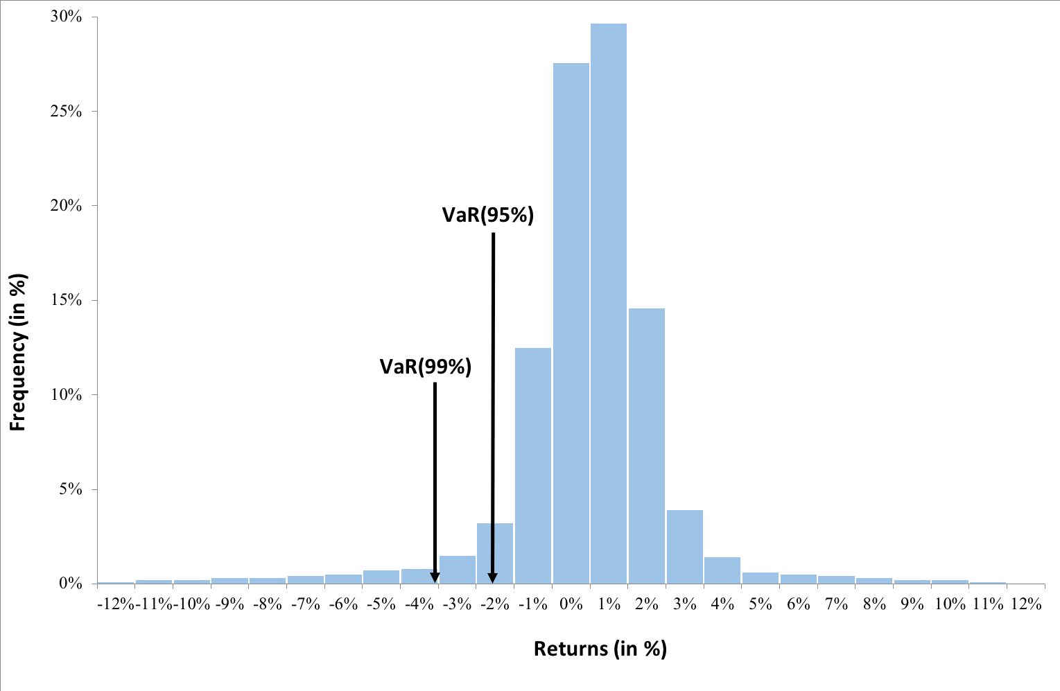
Source: computation by the author.
From the above graph, we can interpret VaR for 99% confidence level as -3% i.e., there is a 99% probability that daily returns we obtain in future are greater than -3%. Similarly, VaR for 95% confidence level as -1.72% i.e., there is a 95% probability that daily returns we obtain in future are greater than -1.72%.
You can download below the Excel file for computation of VaR for CAC40 stock using Monte Carlo method involving GARCH(1,1) model for simulation of returns.

Advantages and limitations of Monte Carlo method for VaR
The Monte Carlo method is a very powerful approach to VAR due its flexibility. It can potentially account for a wide range of scenarios. The simulations also account for nonlinear exposures and complex pricing patterns. In principle, the simulations can be extended to longer time horizons, which is essential for risk measurement and to model more complex models of expected returns.
This approach, however, involves investments in intellectual and systems development. It also requires more computing power than simpler methods since the more is the number of simulations generated, the wider is the range of potential scenarios or outcomes modelled and hence, greater would be the potential accuracy of VaR estimate. In practical applications, VaR measures using Monte Carlo simulation often takes hours to run. Time requirements, however, are being reduced significantly by advances in computer software and faster valuation methods.
Related posts on the SimTrade blog
▶ Jayati WALIA Quantitative Risk Management
▶ Jayati WALIA Value at Risk
▶ Jayati WALIA The historical method for VaR calculation
▶ Jayati WALIA The variance-covariance method for VaR calculation
▶ Jayati WALIA Brownian Motion in Finance
Useful resources
Jorion P. (2007) Value at Risk, Third Edition, Chapter 12 – Monte Carlo Methods, 321-326.
About the author
The article was written in March 2022 by Jayati WALIA (ESSEC Business School, Grande Ecole Program – Master in Management, 2019-2022).