My first experience in corporate finance inside a CAC40 group

September 30, 2021 by Pierre BERGES

My first experience in corporate finance inside a CAC40 group

In this article, Pierre BERGES (ESSEC Business School, Master in Strategy & Management of International Business (SMIB), 2020-2021) shares with us his experience in the Finance Department at Bouygues (a French firm included in the CAC40 index).

About Bouygues

Born in 1952 under the impulsion of Francis Bouygues and now managed by his son Martin, the Bouygues group has become in 70 years a gigantic and well-oiled machine which diversified in many fields along the years such as construction (Bouygues Construction), Telecommunications (Bouygues Telecom), Real Estate (Bouygues Immobilier), Road (Colas) and Media (TF1). Operating in over 80 countries with 129,000 employees, Bouygues is one of the biggest actors of the building industry around the world and the second French building company behind Vinci. As a major actor of the CAC 40 index and because of its numerous actions in M&A (Colas in 1985, TF1 in 1987…), Bouygues has developed a strong financial expertise especially regarding corporate finance.

My experience at Bouygues

My goal as an ESSEC’s student was to develop my skills in finance in order to find a job that will challenge me and help me learn each day, that’s why I chose to search for an internship in corporate finance and, if possible, inside a French historic group. I had the chance to join the team of the Finance Department of Bouygues SA and work with the senior financial managers on two missions. The first mission was to report all the critical financial information of the Bouygues’s subsidiaries to the Chief Financial Officer (CFO) and Top Management Team (TMT) each month and monitor the results of the subsidiaries in order to adapt the strategy in case of unusual results. The second mission was the construction of the rating files dedicated to the two rating agencies, Moody’s and S&P, for the rating of Bouygues. I had also to work on more punctual missions related to Bouygues’s stocks (share buyback, stock options, employees saving plan, protection thought derivatives…).

The process of rating

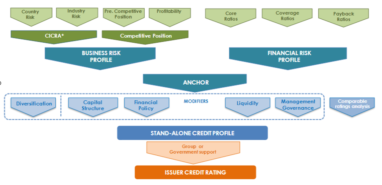
My main mission was to support the managers during the construction of the rating files for the rating agencies Moody’s and S&P. The aim of those files was to help the agencies during their decision process by giving all the information needed under the best light possible to increase or at least maintain the rating of Bouygues. Even though it’s almost impossible for a company to influence the financial aspects of the rating, the company can still work on more flexible aspects of the rating process such as the country risk (risks of the countries where the firm operates), the industry risk (risk of the industry the firm chose to develop). For Bouygues some flexibility is possible regarding the repartition of the earnings coming from media, construction, telecommunication…) or the management governance for example. Our work was to find the best way to optimize those topics and therefore the best way to improve Bouygues’s rating for future market operations.

Figure 1: Structure of the S&P rating.

Source: S&P.

What I’ve learnt during this internship

This internship taught me a lot about corporate finance and how companies use finance to maximize their profits and protect their assets. It also taught me about the central position of rating agencies in the strategy of a company, especially if this company plans to expand through bonds or other financial instruments. Finally, I’ve learnt the way a company can and have to interact with other actors and how the market can influence both the company strategy and its behavior on a daily basis.

Relevance to the SimTrade certificate

The SimTrade certificate is a powerful ally especially regarding the missions linked to Bouygues’s stocks. It allows me to quickly understand the concepts of stock-options or derivative and increase my effectiveness regarding those topics. The certificate is a very good way to learn the basics of financial markets and build on those basics to progress on more complex subjects

Useful resources

Academic articles

Louizi, A., Kammoun, R., 2016. Le positionnement des agences de Notation dans l’évaluation du système de gouvernance d’entreprise, Gestion 2000, 33(5-6):149-175.

Business

Bouygues Presentation and history of Bouygues group

S&P Global

Moody’s

About the author

The article was written in September 2021 by Pierre BERGES (ESSEC Business School, Master in Strategy & Management of International Business (SMIB), 2020-2021).

Smart Beta 1.0

September 23, 2021 by Youssef LOURAOUI

In this article, Youssef LOURAOUI (ESSEC Business School, Global Bachelor of Business Administration, 2017-2021) presents the concept of the smart beta 1.0, the first generation of alternative indexing investment strategies that created a new approach in the asset management industry.

This post is structured as follows: we start by defining smart beta 1.0 as a topic. Finally, we discuss an empirical study by Motson, Clare and Thomas (2017) emphasizing the origin of smart beta.

Definition

The “Smart Beta” expression is commonly used in the asset management industry to describe innovative indexing investment strategies that are alternatives to the market-capitalization-weighted investment strategy (buy-and-hold). In terms of performance, the smart beta “1.0” approach outperforms market-capitalization-based strategies. According to Amenc et al. (2016), the latter have a tendency for concentration and unrewarded risk, which makes them less appealing to investors. In finance, “unrewarded risk” refers to taking on more risk without receiving a return that is commensurate to the increased risk.

When smart beta techniques were first introduced, they attempted to increase portfolio diversification over highly concentrated and capitalization-weighted, as well as to capture the factor premium available in equity markets, such as value indices or fundamentally weighted indices which aim to capture the value premium. While improving capitalization-weighted indices is important, concentrating just on increasing diversity or capturing factor exposure may result in a less than optimal outcome. The reason for this is that diversification-based weighting systems will always result in implicit exposure to certain factors, which may have unintended consequences for investors who are unaware of their implicit factor exposures. Unlike the second generation of Smart Beta, the first generation of Smart Beta are integrated systems that do not distinguish between stock selection and weighting procedures. The investor is therefore required to be exposed to certain systemic risks, which are the source of the investor’s poor performance.

Thus, the first-generation Smart Beta indices are frequently prone to value, small- or midcap, and occasionally contrarian biases, since they deconcentrate cap weighted indices, which are often susceptible to momentum and large growth risk. Furthermore, distinctive biases on risk indicators that are unrelated to deconcentration but important to the factor’s objectives may amplify these biases even further. Indexes that are fundamentally weighted, for example, have a value bias because they apply accounting measures that are linked to the ratios that are used to construct value indexes.

Empirical study: monkeys vs passive mangers

Andrew Clare, Nick Motson, and Steve Thomas assert that even monkey-created portfolios outperform cap-weighted benchmarks in their study (Motson et al., 2017). A lack of variety in cap-weighting is at the foundation of the problem. The endless monkey theory states that a monkey pressing random keys on a typewriter keyboard for an unlimited amount of time will almost definitely type a specific text, such as Shakespeare’s whole works. For 500 businesses, there is an infinite number of portfolio weighting options totaling 100%; some will outperform the market-capitalization-weighted index, while others will underperform. The authors of the study take the company’s ticker symbol and use the following guidelines to create a Scrabble score for each stock:

A, E, I, O, U, L, N, S, T, R – 1 point. D and G both get two points.
B, C, M, P – 3 points ; F, H, V, W, Y – 4 points ; K – 5 points.
J, X – 8 points ; Q, Z – 10 points

The scores of each company’s tickers are then added together and divided by this amount to determine each stock’s weight in the index. As illustrated in Figure 1, the results obtained are astonishing, resulting in a clear outperformance of the randomly generated portfolios compared to the traditional market capitalization index by 1.5% premium overall.

Figure 1. Result of the randomly generated portfolio with the Cass Scrabble as underlying rule compared to market-capitalization portfolio performance.
Scrabble_performance
Source: Motson et al. (2017).

In the same line, the authors produced 500 weights that add up to one using this technique, with a minimum increase of 0.2 percent. The weights are then applied to a universe of 500 equities obtained from Bloomberg in December 2015 (Motson et al., 2017). The performance of the resultant index is then calculated over the next twelve months. This technique was performed ten million times. As illustrated in Figure 2, the results are striking, with smart beta funds outperforming nearly universally in the 10 million simulations run overall, and with significant risk-adjusted return differences (Motson et al., 2017).

Figure 2. 10 million randomly generated portfolios based on a portfolio construction of 500 stocks
Scrabble_performance
Source: Motson et al. (2017).

For performance analysis, the same method was employed, but this time for a billion simulation. This means they constructed one billion 500-stock indexes with weights set at random or as if by a monkey. Figure 9 suggests that the outcome was not accidental. The black line shows the distribution of 1 billion monkeys’ returns in 2016, while the grey line shows the cumulative frequency. 88 percent of the monkeys outperformed the market capitalization benchmark, according to the graph. The luckiest monkey returned 27.2 percent, while the unluckiest monkey returned just 3.83 percent (Motson et al., 2017) (Figure 3).

FFigure 3. Result of one billion randomly simulated portfolios based on a portfolio construction of 500 stocks.
Scrabble_performance
Source: Motson et al. (2017).

Why should I be interested in this post?

If you are a business school or university undergraduate or graduate student, this content will help you in understanding the various evolutions of asset management throughout the last decades and in broadening your knowledge of finance.

If you’re an investor, you’re probably aware that smart beta funds have become a popular topic. Smart beta is a game-changing development that fills a gap in the market for investors: a better return for a reduced risk, net of transaction and administrative costs. These strategies, in a sense, establish a new market. As a result, smart beta is gaining traction and having an impact on asset management.

Useful resources

Academic research

Amenc, N., F., Goltz, F. and Le Sourd, V., 2016. Investor perception about Smart beta ETF. EDHEC Risk Institute working paper.

Amenc, N., F., Goltz, F. and Martinelli, L., 2013. Smart beta 2.0. EDHEC Risk Institute working paper.

Motson, N., Clare, A. & Thomas, S., 2017. Was 2016 the year of the monkey?. Cass Business School research paper.

About the author

The article was written in September 2021 by Youssef LOURAOUI (ESSEC Business School, Global Bachelor of Business Administration, 2017-2021).

Alternative to market-capitalization weighting strategies

September 23, 2021 by Youssef LOURAOUI

In this article, Youssef LOURAOUI (ESSEC Business School, Global Bachelor of Business Administration, 2017-2021) presents the different alternatives developed to the market-capitalization weighting strategy (buy-and-hold strategy).

The structure of this post is as follows: we begin by introducing alternatives to market capitalization strategies as a topic. We then will delve deeper by presenting heuristic-based weighting and optimization-based weighting strategies.

Introduction

The basic rule of applying a market-capitalization weighting methodology for the development of indexes has recently come under fire. As the demand for indices as investment vehicles has grown, different weighting systems have emerged. There have also been a number of recent projects for non-market-capitalization-weighted ETFs. Since the first basic factor weighted ETF was released in May 2000, a slew of ETFs has been released to monitor non-market-cap-weighted indexes, including equal-weighted ETFs, minimal variance ETFs, characteristics-weighted ETFs, and so on. These are dubbed “Smart Beta ETFs” since they aim to outperform traditional market-capitalization-based indexes in terms of risk-adjusted returns (Amenc et al. 2016).

The categorization approach will be the same as Chow, Hsu, Kalesnik, and Little (2011), with the following distinctions: 1) basic weighting techniques (heuristic-based weighting) and 2) more advanced quantitative weighting techniques (optimization-based weighting).

It’s an arbitrary categorization system designed to make reading easier by differentiating between simpler and more complicated approaches.

Heuristic-based weighting strategies

Equal-weighting

The equal weighting method assigns the same weight to each share making up the portfolio (or index)

Where w_i represents the weight of asset i in the portfolio and N the total number of assets in the portfolio.

Because each component of the portfolio has the same weight, equal weighting helps investors to obtain more exposure to smaller firms. Bigger firms will be more represented in the market-capitalization-weighted portfolio since their weight will be larger. The benefit of this technique is that tiny capitalization risk-adjusted-performance tends to be better than big capitalization (Banz, 1981).

In their study, Arnott, Kalesnik, Moghtader, and Scholl (2010) created three distinct indices in terms of index composition. The first group consists of enterprises with substantial market capitalization (as are capitalisation-weighted indices). Each business in the index is then given equal weight. This is how the majority of equally-weighted indexes are built (MSCI World Equal Index, S&P500 Equal Weight Index). The second is to create an index based on basic criteria and then assign equal weight to each firm. The third strategy is a hybrid of the first two. It entails averaging the ranks from the two preceding approaches and then assigning equal weight to the remaining 1000 shares.

Fundamental-weighting

The weighting approach based on fundamentals divides companies into categories based on their basic size. Sales, cash flow, book value, and dividends are all taken into account. These four parameters are used to determine the top 1,000 firms, and each firm in the index is given a weight based on the magnitude of their individual components (Arnott et al., 2005). The portfolio weight of the _ith stock is defined as:

For a fundamental index that includes book value as a consideration, for example, the top 1,000 companies in the market with the most extensive book values are chosen. Firm x_i is given a weight w_i, which is equal to the firm’s book value divided by the total of the index components’ book values.

Fundamental indexation tries to address the following bias: in a cap-weighted index, if the market efficiency hypothesis is not validated and a share’s price is, for example, overpriced (greater than its fair value), the share’s weight in the index will be too high. Weighting by fundamentals will reduce the bias of over/underweighting over/undervalued companies based on criteria like sales, cash flows, book value, and dividends, which are not affected by market opinion, unlike capitalization.

Low beta weighting

Low-beta strategies are based on the fact that equities with a low beta have greater returns than those expected by the CAPM (Haugen and Heins, 1975). A beta of less than one indicates that the share price has tended to grow less than its benchmark index during bullish trends and to decrease less severely during negative trends throughout the observed timeframe. A low-beta index is created by selecting low-beta stocks and then giving each stock equal weight in the index. As a result, it’s a hybrid of a low-beta and an equal-weighting method. On the other side, high beta strategies enable investors to profit from the amplification of favourable market moves.

Reverse-capitalization weighting

The weight of an asset capitalization-weighted index can be defined as:

where MC stands for “Market Capitalization”, and w_i is the weight of asset i in the portfolio.

In a reverse market-capitalization-weighted index, the weight of an asset is defined as:

“Reverse market-capitalization” is abbreviated as RMC. This technique necessitates using a cap-weighted index to execute the approach. RCW methods, like equal-weight or low-beta strategies, are motivated by the fact that small caps have a greater risk-adjusted return than big caps. This sort of indexation requires constant rebalancing (Banz, 1981).

Maximum diversification

This technique aims to build a portfolio with as much diversification as feasible. A diversity index (DI) is employed to achieve the desired outcome, which is defined as the distance between the sum of the constituents’ volatilities and the portfolio’s volatility (Amenc, Goltz, and Martellini, 2013). Diversity weighting is one of the better-known portfolio heuristics that blend cap weighting and equal weighting. Fernholz (1995) defined stock market diversity, D_p, as

where p between (0,1) and x _Market,i is the weight of the _ith stock in the cap-weighted market portfolio, and then proposed a strategy of portfolio weighting whereby portfolio weights are defined as

where i = 1, . . . , N; p between (0,1); and the parameter p targets the desired level of portfolio tracking error against the cap-weighted index.

Optimization-based weighting strategies

The logic of Modern Portfolio Theory (Markowitz, 1952) is followed in Mean-Variance optimization. Theoretically, if we know the expected returns of all stocks and their variance-covariance matrix, we can construct risk-adjusted-performance optimal portfolios. However, these two inputs for the model are difficult to estimate precisely in practice. Chopra and Ziemba (1993) showed that even little inaccuracies in these parameters’ estimates may have a large influence on risk-adjusted-performance.

Minimum Variance

Chopra and Ziemba (1993) adopt the simple premise that all stocks have the same return expectation, based on the fact that stock return expectations are difficult to quantify. As a result of this premise, the best portfolio is the one that minimizes risk. The goal of minimal variance strategies, which have been around since 1990, is to provide a better risk-return profile by lowering portfolio risk without modifying return expectations. The low volatility anomaly justifies this technique. Low-volatility stocks have historically outperformed high-volatility equities. These portfolios are built without using a benchmark as a guide. The portfolio variance minimization equation for a two-asset portfolio is as follows:

In their research on the construction of this type of index, Arnott, Kalesnik, Moghtader and Scholl (2010) found that risk measures that take into account interest rates, oil prices, geographical region, sector, size, expected return, and growth, as calculated by the Northfield global risk model, a model for making one-year risk forecasts, reduce the portfolio’s absolute risk. This method is used in the MSCI World Minimum Volatility Index, which was released in 2008.

Global Minimum Variance, Maximum Decorrelation, and Diversified Minimum Variance are the three types of minimum variance techniques (Amenc, Goltz and Martellini, 2013). However, there are no indexes or exchange-traded funds (ETFs) based on the Maximum Decorrelation and Diversified Minimum Variance methods in actuality; they are still only theoretical notions.

Maximum Sharpe ratio

Because all stocks are unlikely to have the same expected returns, the minimum-variance portfolio—or any practical representation of its concept—is unlikely to have the highest ex-ante Sharpe ratio. Investors must incorporate useful information about future stock returns into a minimum-variance approach to improve it. Choueifaty and Coignard (2008) proposed a simple linear relationship between the expected premium, E(R_i) – R_f, for a stock and its return volatility, sigma_i:

A related portfolio method proposed by Amenc, Goltz, Martellini, and Retkowsky (2010) implies that a stock’s expected returns are linearly related to its downside semi-volatility. They claimed that portfolio losses are more important to investors than gains. As a result, rather than volatility, risk premium should be connected to downside risk (semi-deviation below zero). The EDHEC-Risk Efficient Equity Indices are built around this assumption. Downside semi-volatility can be defined mathematically as

where R_{i, t} is the return for stock _i in period _t.

Maximum Sharpe ratio can be considered as an alternative beta technique that aims to solve the challenges of forecasting risks and returns for a large number of equities.

Why should I be interested in this post?

Smart beta funds have become a hot issue among investors in recent years. Smart beta is a game-changing invention that addresses an unmet need among investors: a higher return for lower risk, net of transaction and administrative costs. In a way, these investment strategies create a new market. As a result, smart beta is gaining traction and influencing the asset management industry.

Useful resources

Academic research

Amenc, Noël, Felix Goltz, Lionel Martellini, and Patrice Ret- kowsky. 2010. “Efficient Indexation: An Alternative to Cap- Weighted Indices.” EDHEC-Risk Institute (February).

Amenc, N., Goltz, F., Le Sourd, V., 2016. Investor perception about Smart beta ETF. EDHEC Risk Institute working paper.

Amenc, N., Goltz, F., Martinelli, L., 2013. Smart beta 2.0. EDHEC Risk Institute working paper.

Arnot, R.D., Hsu, J., Moore, P., 2005. Fundamental Indexation. Financial Analysts Journal, 61(2):83-98.

Arnot, R.D., Kalesnik, V., Moghtader, P., Scholl, S., 2010. Beyond Cap Weight, The empirical evidence for a diversified beta. Journal of Indexes, January, 16-29.

Banz, R., 1981. The relationship between return and market value of common stocks. Journal of Financial Economics. 9(1):3-18.

Chopra, V., Ziemba, W., 1993. The Effect of Errors in Means, Variances, and Covariances on Optimal Portfolio Choice. Journal of Portfolio Management, 19:6-11.

Chow, T., Hsu, J., Kalesnik, V., Little, B., 2011. A Survey of Alternative Equity Index Strategies. Financial Analyst Journal, 67(5):35-57.

Choueifaty, Yves, and Yves Coignard. 2008. Toward Maximum Diversification. Journal of Portfolio Management, vol. 35, no. 1 (Fall):40–51.

Fernholz, Robert. 1995. Portfolio Generating Functions. Working paper, INTECH (December).

Haugen, R., Heins, J., 1975. Risk and Rate of Return of Financial Assets: Some Old Wine in New Bottles. Journal of Financial and Quantitative Analysis, 10(5):775-784.

Markowitz, H., 1952. Portfolio Selection. The Journal of Finance, 7(1):77-91.

About the author

The article was written in September 2021 by Youssef LOURAOUI (ESSEC Business School, Global Bachelor of Business Administration, 2017-2021).

Markowitz Modern Portfolio Theory

January 30, 2024September 20, 2021 by Youssef LOURAOUI

Markowitz Modern Portfolio Theory

In this article, Youssef LOURAOUI (ESSEC Business School, Global Bachelor of Business Administration, 2017-2021) presents Markowitz’s Modern Portfolio Theory, a pioneering framework for understanding the impact of the number of stocks in a portfolio and their covariance relationships on portfolio diversification.

We begin by presenting Markowitz’s Modern Portfolio Theory (MPT) as the origin of factor investing (market factor). The assumptions of the model are then discussed. We’ll go through some of the model’s fundamental concepts next. We wrap up with a discussion of the concept’s limitations and a general conclusion.

Modern Portfolio Theory

The work conducted by Markowitz is widely acknowledged as a pioneer in financial economics and corporate finance for his theoretical implications and its application in financial markets. In 1990, Markowitz shared the Nobel Prize for his contributions to these domains, which he articulated in his 1952 article “Portfolio Selection” published in The Journal of Finance. His seminal work laid the groundwork for what is now often referred to as ‘Modern Portfolio Theory’ (MPT).

Modern portfolio theory was first introduced by the work of Harry Markowitz in 1952. Overall, the risk component of MPT can be quantified using various mathematical formulations and mitigated through the concept of diversification, which entails carefully selecting a weighted collection of investment assets that collectively exhibit lower risk characteristics than any single asset or asset class. Diversification is, in fact, the central notion of MPT and is predicated on the adage “never put all your eggs in one basket”.

Assumptions of the Markowitz Portfolio Theory

MPT is founded on several market and investor assumptions. Several of these assumptions are stated explicitly, while others are implied. Markowitz’s contributions to MPT in portfolio selection are based on the following basic assumptions:

Investors are rational (they seek to maximize returns while minimizing risk).
Investors will accept increased risk only if compensated with higher expected returns.
Investors receive all pertinent information regarding their investment decision in a timely manner.
Investors can borrow or lend an unlimited amount of capital at a risk-free rate of interest.

Concepts used in the MPT

Risk

Risk is equivalent to volatility in Markowitz’ portfolio selection theory—the larger the portfolio volatility, the greater the risk. Volatility is a term that refers to the degree of risk or uncertainty associated with the magnitude of variations in a security’s value. Risk is the possibility that an investment’s actual return will be less than predicted, which is technically quantified by standard deviation. A larger standard deviation implies a bigger risk and, hence, a larger potential return. If investors are prepared to take on risk, they anticipate earning a risk premium. Risk premium is defined as “the expected return on an investment that exceeds the risk-free rate of return”. The bigger the risk, the more risk premium investors need.”. Riskier investments do not necessarily provide a higher rate of return than risk-free ones. This is precisely why they are hazardous. However, historical evidence suggests that the only way for investors to obtain a better rate of return is to take on greater risk.

Systematic risk

Systematic risk is a type of risk at the macroeconomic level—risk that impacts a large number of assets to varying degrees. Inflation, interest rates, unemployment rates, currency exchange rates, and Gross National Product levels are all instances of systematic risk variables. These economic conditions have a significant influence on practically all securities. As a result, systemic risk cannot be completely eradicated.

Unsystematic risk

Unsystematic risk (or specific risk), on the other hand, is a type of risk that occurs at the micro-level risk factors that influence only a single asset or a small group of assets. It entails a distinct risk that is unrelated to other hazards and affects only particular securities or assets. For instance, Netflix’s poorly accepted adjustment to its planned consumer pricing structure elicited an extraordinarily unfavorable consumer response and defections, resulting in decreased earnings and stock prices. However, it had little effect on the Dow Jones or S&P 500 indexes, or on firms in the entertainment and media industries in general—with the probable exception of Netflix’s largest rival Blockbuster Video, whose value grew dramatically as a result of Netflix’s declining market share. Additional instances of unsystematic risk include a firm’s credit rating, poor newspaper coverage of a corporation, or a strike impacting a specific company. Diversification of assets within a portfolio can greatly minimize unsystematic risk.

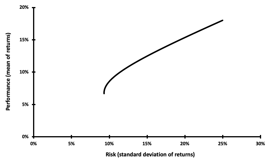
Because the returns on various assets are, in fact, connected to some extent, unsystematic risk can never be totally avoided regardless of the number of asset classes pooled in a portfolio. The Markowitz Efficient Frontier is depicted in Figure 1, with all efficient portfolios on the upper line. The efficient frontier is a set of optimal portfolios that offer the best-projected return for a specified level of risk, or the lowest risk for a specified level of return. Portfolios that fall below the efficient frontier are inefficient because they do not generate a sufficient rate of return in relation to the level of risk (Figure 1).

Figure 1. Markowitz Efficient Frontier.

Source: computations by the author.

Risk-return trade-off

The term risk-return trade-off refers to Markowitz’s fundamental theory that the riskier an investment, the larger the necessary potential return (or expected return). Investors will generally retain a hazardous investment only if the predicted return is sufficiently high to compensate them for taking the risk. Markowitz derives a relation between expected return (μ) and variance (σ²_p) captured in the following expression. Refer to the post Implementation of the Markowitz allocation model for a better understanding of the mathematical foundations of this approach:

img_SimTrade_variance_Markowitz_portfolio

where

A, B and C = Optimization parameters
μ = expected return vector

Diversification

The words ‘diversification’ and ‘Diversification Effect’ relate to the correlations between portfolio risk and diversification. Diversification, a tenet of Markowitz’s portfolio selection theory and MPT, is a risk-reduction strategy that entails allocating assets among a variety of financial instruments, sectors, and other asset classes. In more straightforward terms, it refers to the aphorism “don’t put all your eggs in one basket.” If the basket is dropped, all eggs are shattered; if many baskets are used, the likelihood of all eggs being destroyed is significantly decreased. Diversification may be accomplished by investments in a variety of companies, asset types (e.g., bonds, real estate, etc.), and/or commodities such as gold or oil.

Diversification seeks to enhance returns while minimizing risk by investing in a variety of assets that will react differently to the same event (s). For example, whenever there is unfavorable news about the European debt crisis, the stock market typically declines dramatically. Simultaneously, the same news has generally benefited the price of specific commodities, such as gold. As a result, portfolio diversification methods should include not just diverse stocks inside and outside of the same industry, but also diverse asset classes, such as bonds and commodities. The Diversification Effect is a term that relates to the link between portfolio correlations and diversification. When there is an imperfect connection between assets (positive or negative), the diversification effect occurs. It is a critical and successful risk mitigation method since risk mitigation may be accomplished without jeopardizing profits. As a result, any prudent investor who is ‘risk cautious’ will diversify to a certain extent.

Limitation of the model

Despite its monumental theoretical significance, MPT has a slew of opponents who contend that its underlying assumptions and modeling of financial markets are frequently out of step with reality. One could argue that none of them are totally accurate and that each of them undermines MPT to varied degrees. Generally, some of the most common complaints include the following: irrationality of investors, relation between risk and return, treatment of information by investors, limitless borrowing capacity, perfectly efficient markets, and no taxes or transaction costs.

Irrationality of investors

It is assumed that investors are rational and aim to maximize returns while reducing risk. This is contrary to what market participants who become swept up in ‘herd behavior’ investment activity observe. For example, investors frequently gravitate into ‘hot’ industries, and markets frequently boom or burst because of speculative excesses.

Relation between risk and expected return

Increased risk = Increased expected returns. The idea that investors will only take more risk in exchange for higher predicted profits is regularly refuted by investor behavior. Frequently, investing techniques need investors to make a perceived hazardous investment (e.g., derivatives or futures) in order to lower total risk without increasing projected profits significantly. Additionally, investors may have certain utility functions that override worries about return distribution.

Treatment of information by investors

MPT anticipates that investors will get all information pertinent to their investment in a timely and thorough manner. In fact, global markets are characterized by information asymmetry (one party possesses superior knowledge), insider trading, and investors who are just more knowledgeable than others. This may explain why stocks, commercial assets, and enterprises are frequently acquired at a discount to their book or market value.

Limitless Borrowing Capacity

Another critical assumption mentioned previously is that investors have nearly unlimited borrowing capacity at a risk-free rate. Each investor has credit constraints in real-world markets. Additionally, only the federal government may borrow at the zero-interest treasury bill rate on a continuous basis.

Perfectly efficient markets

Markowitz’s theoretical contributions to MPT are predicated on the premise that markets are perfectly efficient (Markowitz, 1952). On the other hand, because MPT is based on asset values, it is susceptible to market whims such as environmental, personal, strategic, or social investment choice factors. Additionally, it ignores possible market failures like as externalities (costs or benefits that are not reflected in pricing), information asymmetry, and public goods (a non-rivalrous and non-excludable item). From another vantage point, centuries of ‘rushes’, ‘booms’, ‘busts’, ‘bubbles’, and ‘market crises’ illustrate that markets are far from efficient.

No Taxes or Transaction Costs

Neither taxes nor transaction costs are included in Markowitz’ theoretical contributions to MPT. To the contrary, genuine investment products are subject to both taxes and transaction costs (e.g., broker fees, administrative charges, and so on), and considering these costs into portfolio selection may certainly affect the optimal portfolio composition.

Conclusion

MPT has become the de facto dogma of contemporary financial theory and practice. The idea of MPT is that beating the market is tough, and those that do do it by diversifying their portfolios properly and taking above-average investing risks. The critical point to remember is that the model is only a tool—albeit the most powerful hammer in one’s financial toolbox. It has been over sixty years since Markowitz introduced MPT, and its popularity is unlikely to decrease anytime soon. His theoretical insights have served as the foundation for more theoretical investigation in the field of portfolio theory. Nonetheless, Markowitz’s portfolio theory is susceptible to and dependent on ongoing ‘probabilistic’ development and expansion.

Why should I be interested in this post?

Modern Portfolio Theory is at the heart of modern finance and its core foundations are structuring the modern investing panorama. MPT has established itself as the foundation for modern financial theory and practice. MPT’s premise is that beating the market is difficult, and those that do it by diversifying their portfolios appropriately and accepting higher-than-average investment risks.

MPT has been around for almost sixty years, and its popularity is unlikely to wane anytime soon. His theoretical contributions have laid the groundwork for more theoretical research in the field of portfolio theory. Markowitz’s portfolio theory, however, is vulnerable to and dependent on continuing ‘probabilistic’ development and expansion.

Useful resources

Academic research

Ang, A., 2013. Factor Investing. Working paper.

Mangram, M.E., 2013. A simplified perspective of the Markowitz Portfolio Theory. Global Journal of Business Research, 7(1): 59-70.

Markowitz, H., 1952. Portfolio Selection. The Journal of Finance, 7(1): 77-91.

Mossin, J. 1966. Equilibrium in a Capital Asset Market. Econometrica, 34(4): 768-783.

Sharpe, W.F. 1963. A Simplified Model for Portfolio Analysis. Management Science, 9(2): 277-293.

Sharpe, W.F. 1964. Capital Asset Prices: A Theory of Market Equilibrium under Conditions of Risk. The Journal of Finance, 19(3): 425-442.

About the author

The article was written in September 2021 by Youssef LOURAOUI (ESSEC Business School, Global Bachelor of Business Administration, 2017-2021).

Smart Beta strategies: between active and passive allocation

September 20, 2021 by Youssef LOURAOUI

Smart Beta strategies: between active and passive allocation

In this article, Youssef LOURAOUI (ESSEC Business School, Global Bachelor of Business Administration, 2017-2021) discusses the topic of smart beta strategies and especially the debate about its position as an active or passive allocation.

Smart beta strategies appear to be in the middle of the polarized asset management industry, which is segmented between active investing based on beating the performance of a given benchmark, and passive investing based on replicating a given benchmark.

This article is structured as follows: we begin by introducing the topic of smart beta strategies. We then discuss the different investing approach and their characteristic. A simple simulation exercise is then presented to understand how an alternative to market-capitalization-weightings indexes leads to different results. We wrap up with a general conclusion of the topic.

Introduction

Smart beta strategies are often found somewhere in the middle between active and passive investment management. In this post, we look at how investors think about this characteristic of smart beta investment strategies.

Passive funds aim at replicating or tracking an index (such as the S&P500 index in the US or the CAC40 index in France for equity markets) use a buy-and-hold strategy to achieve their goal of mimicking the performance of the market index. The beta of a passive fund is very close to the beta of the market index (benchmark).

Active funds are supervised by a portfolio manager that screens the best investments for the fund and time the market to profit from an upside potential. The excess return over the performance of the market index (benchmark) is referred to as alpha.

Smart beta funds are justified by the fact that capitalization-weighted strategies appear to be inefficient. They are based on transparent and rule-based strategies. Investors seek to obtain additional factor betas to enhance their portfolio performance.

While passive investing aims to match the market return, and active strategies rely on the fund manager’s ability to outperform the market, smart beta can be seen as a hybrid of the two approaches, with a passive component in the sense that it tracks one or more factors that are transparent and rule-based, and an active component in which the portfolio is managed, that is to say, rebalanced from time to time. Table 1 describes the main types of funds (passive, active and smart beta) and their respective strategies according to the investment approach and asset allocation methodology, and performance metrics. We also indicate the Greek letter that each strategy.

Table 1. Description of the main types of funds and their respective strategies.

Source: table done by the author.

The passive investing approach

The Efficient Market Hypothesis (EMH) asserts that markets are efficient. The passive investing strategy is built on the concept of “buy-and-hold,” or keeping an investment position for a lengthy period without worrying about market timing or acting on the bought position. This latter technique is frequently implemented through the purchase of exchange-traded funds (ETF) that aim to closely match a given benchmark to produce a performance that is comparable to the underlying index or benchmark. The index might be broad-based, such as the S&P500 index in the US equity market for instance, or more specialized, such as an index that monitors a specific sector or geographical zone.

The active investing approach

Active management is an approach for going beyond matching a benchmark’s performance and instead aiming to outperform it. The alpha may be calculated using the same CAPM model framework, by linking the expected return with the fund manager’s extra return on the portfolio’s overall performance (Jensen, 1968). The search for alpha is done through two very different types of investment approaches: stock picking and market timing.

Stock picking

Stock picking is a method used by active managers to select assets based on a variety of variables such as their intrinsic value, the growth rate of dividends, and so on. Active managers use the fundamental analysis approach, which is based on the dissection of economic and financial data that may impact the asset price in the market.

Market timing

Market timing is a trading approach that involves entering and exiting the market at the right time. In other words, when rising outlooks are expected, investors will enter the market, and when downward outlooks are expected, investors will exit. For instance, technical analysis, which examines price and volume of transactions over time to forecast short-term future evolution, and fundamental analysis, which examines the macroeconomic and microeconomic data to forecast future asset prices, are the two techniques on which active managers base their decisions.

Review of academic literature

Passive investing

We can retrace the foundations of passive investing to the theory of portfolio construction developed by Harry Markowitz. For his theoretical implications, Markowitz’s work is widely regarded as a pioneer in financial economics and corporate finance. For his contributions to these disciplines, which he developed in his thesis “Portfolio Selection” published in The Journal of Finance in 1952. Markowitz received the Nobel Prize in economics in 1990. His groundbreaking work set the foundation for what is now known as ‘Modern Portfolio Theory’ (MPT).

William Sharpe, John Lintner, and Jan Mossin separately developed The Capital Asset Pricing Model (CAPM) as a result of Markowitz past research. The CAPM was a huge evolutionary step forward in capital market equilibrium theory because it enabled investors to appropriately value assets in terms of systematic risk. The portfolio management industry intended to capture the market portfolio return in the late 1970s, defined as a hypothetical collection of investments that contains every kind of asset available in the investment universe, with each asset weighted in proportion to its overall market participation. A market portfolio’s expected return is the same as the market’s overall expected return. But as financial research evolved and some substantial contributions were made, new factor characteristics emerged to capture some additional performance.

Active investing

As fund managers tried strategies to beat the market, financial literature delved deeper into the mechanism to achieve this purpose. Jensen’s groundbreaking work in the early ’70s gave rise to the concept of alpha in the tracking of a fund’s performance to distinguish between the fund’s manager’s ability to generate abnormal returns and the part of the returns due to luck (Jensen, 1968).

Smart beta / factor investing

Smart beta is defined as strategies that aim to address the inefficiencies of market capitalization weight indexation. In the early 2000s, as a result of numerous financial publications delving deeper into various elements that gave additional returns to increase the overall performance of the portfolio (the “Fama-French” papers), smart beta strategies evolved. Fund managers develop investment strategies based on researched factors that provide a time-tested abnormal return in exchange for taking on risk.

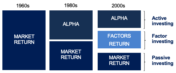
Understanding portfolio returns is crucial to determining how to evaluate portfolio performance. It all stems from Harry Markowitz’s groundbreaking work and pioneering research on portfolio construction and the impact of diversification in improving portfolio performance. Throughout the 1960s and 1970s, investors made no distinction between the sources of portfolio returns. Finance research in the 1980s boosted the popularity of passive investment as an alternate basis for implementation. Investors began to successfully capture market beta through passive strategies. In the 2000s, investors began to see factors as major determinants of long-term return (Figure 1).

Figure 1. Overview of the evolution of performance metrics.

Source: MSCI Factor Research (2021).

Grossman and Stiglitz’s research addressed the limitations of passive investment (1980). If the fund manager actively selects assets for his portfolio rather than passively replicating the benchmark, he may get higher abnormal returns. The term “abnormal returns” refers to the disparity between the actual and projected returns. In the financial literature, this “extra return” is referred to as alpha. It is one of the most tracked performance indicators by fund managers. Grossman and Stiglitz establish that there is no such thing as a successful passive investment. Indeed, they said that the benchmark is composed of assets chosen based on certain criteria (capitalization, return, liquidity, and the weight of each asset in the sector), and that “passive investing” is the most cost-effective alternative to active investing.

As pointed out by Jensen (1968), when assembling a portfolio, there are two points to bear in mind. The first point is the fund manager’s ability to foresee the asset’s price movement, and the second point is the fund manager’s capacity to limit investment risk via diversification.

Case study: Comparison of market-capitalization-weighted portfolios and equally-weighted portfolios

The difference between two investment strategies can be evaluated by comparing the weights of the assets of their associated portfolio. Note that over time the weights can evolve with voluntary sales and purchases of the assets. Such divestments and investments refer to the rebalancing of the portfolio.

Buy-and-hold investing is a passive investment strategy in which an investor buys assets and holds them for a long period, independent of market fluctuations. A buy-and-hold investor selects companies but is indifferent to short-term market swings or technical indicators. The buy-and-hold investment strategy corresponds to market-capitalization-weighted portfolios.

The buy-and-hold approach is recommended by several prominent investors, like Warren Buffett, to individuals seeking profitable long-term returns. Buy-and-hold investors outperform active management on average over longer time horizons and after costs. Buy-and-hold investors, on the other hand, may not sell at the greatest price available, according to proponents.

Excel file for market-capitalization-weighted and equally-weighted portfolios

You can download an Excel file with data used for this exercise.

The goal of this exercise is to compare the performance of the two types of investments and to balance the two approaches to obtain a better understanding of each strategy and its market behavior. To be able to homogeneously analyze the underlying assets of the buy and hold strategy as well as the smart beta approach, three stocks have been simulated.

All the price data, number of shares, stock returns, and market-capitalization are all simulated for a more simplistic model. The buy and hold strategy is based on an evenly weighted portfolio. Only the small-cap stock (Stock 1) will have prices fluctuations to analyze the size effect as a driver of returns in a portfolio. A rebalancing exercise is implemented for the smart beta portfolio, no trading nor any related cost for implementing the strategy is applied and thus, don’t reflect the full picture as in financial markets.

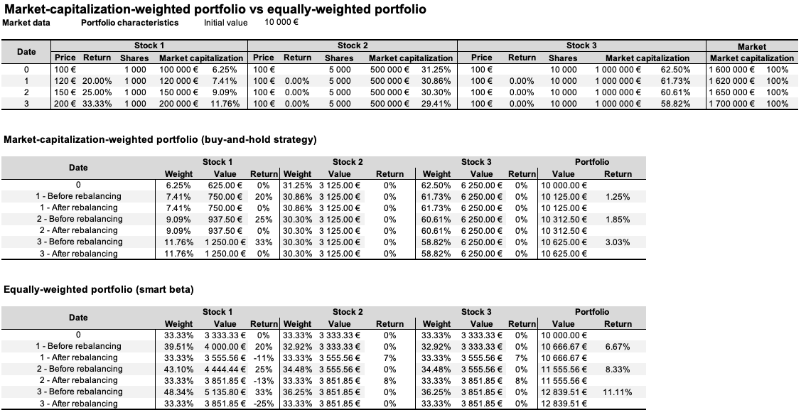
Table 2 is made of three components. The first section of the table represents our data for the simulation. Each stock has a different size representing respectively a small, mid, and large-capitalization firm. Market capitalization is obtained through a simple computation by multiplying the number of shares times the price of each share. The second section of the table is the simulation of a market-capitalization-weighted portfolio. The third section represents a smart beta portfolio that uses an equally-weighted weighting indexing (Table 2). Note that with the market-capitalization-weighted portfolio there is a concentration in the stock with the largest market capitalization (due to its high past performance). An equally-weighted portfolio obtained with rebalancing (often associated with smart beta strategies such as growth) would not present such property and show a more diversified portfolio over time. Note that the frequency of rebalancing the portfolio can affect the risk/performance characteristics. Amenc et. al. (2016) show that the Sharpe ratio tends to decrease with a higher frequency for rebalancing.

Table 2. Simulation of a market-capitalization-weighted portfolio and an equally-weighted portfolio.
Smart_beta_simulation_spreadsheet
Source: simulations and calculations by the author.

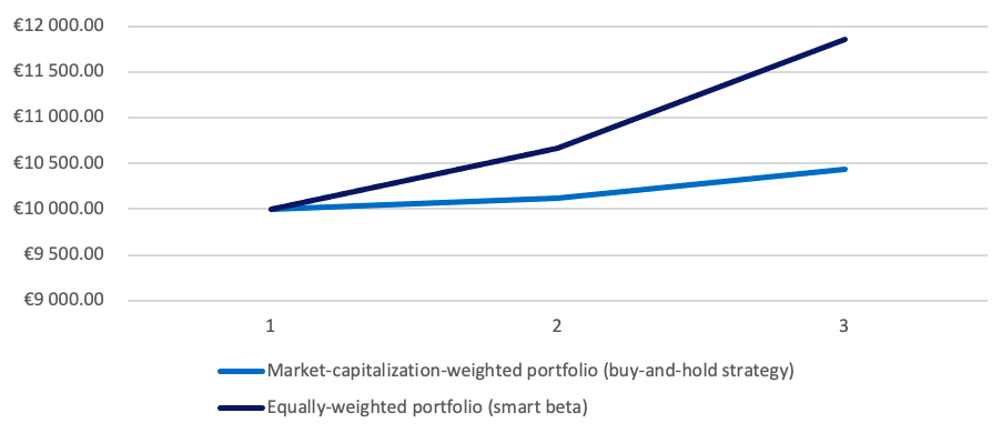
The simulation unveiled that the market-capitalization-weighted portfolio’s size anomaly failed to capture the outperformance of small-cap stocks, resulting in results that were lower than those of the smart beta equally weighted portfolio, which had a good exposure to small caps (Figure 2). The key point of this simulated model is that the market-cap indexation has a defect related to the concentration of large companies in the profile of small caps which represent a small percentage of the index. The size factor is based on a risk factor that aims to capture the documented outperformance of small-cap firms compared to larger enterprises. With this simulated model, we have proven with a very simple model in the conception that the size anomaly can indeed be a vector of return, as researched in the paper of Banz (1981) which precisely describes this concept on the US equity market (Figure 2).

Figure 2. market-capitalization-weighted portfolio vs equally-weighted portfolio.

Source: simulations and calculations by the author.

One aspect to consider in this case analysis is that one of the possible explanations for this outperformance is that the weights are changed at rebalancing dates rather than allowed to drift with the price fluctuations, which is a clear distinction between cap-weighted indexes and smart beta strategies. Some claim that this rebalancing completely explains the success of smart beta strategies (Amenc et al, 2016). This allegation, however, does not hold up under investigation. An examination of buy-and-hold portfolios vs portfolios rebalanced at various frequencies reveals that whether or not rebalancing improves performance is dependent on the return behavior of the assets in the portfolio. Rebalancing may or may not provide better results than buy-and-hold tactics (Amenc et. al., 2016).

Even if beneficial rebalancing impacts occur, Smart Beta methods may not be able to capture them. Contrary to popular belief, data shows that rebalancing an equal-weighted approach more frequently does not always increase performance. Furthermore, both short- and long-term reversal effects are empirically insignificant in explaining the performance of a wide variety of Smart Beta strategies. Naturally, rebalancing is necessary, especially to maintain diversity and target factor exposures. Rebalancing, on the other hand, is not an experimentally verified source of Smart Beta strategy performance (Amenc et. al., 2016).

Smart beta: passive or active investment strategy?

Smart beta investing is considered a hybrid strategy because it attempts to replicate the performance of a predetermined benchmark without engaging in market timing or stock picking, and an active strategy because investors choose to gain exposure to specific factors (beyond the market factor) by rebalancing the portfolio according to some rules. In practice, smart beta strategies often imply rebalancing to maintain target weights for each factor. In this sense, smart beta strategies are active, or at least more active than the buy-and-hold strategy. However, the rebalancing of portfolios of smart beta strategies is usually done with a predefined rule. In this sense, smart beta strategies are passive, or at least more passive than discretionary investment strategies based on stock picking and market timing.

Why should I be interested in this post?

Smart beta funds have become a hot issue among investors in recent years. Smart beta is a game-changing invention (or just a new marketing idea?) that addresses an unmet need among investors: a higher return for lower risk, net of transaction and administrative costs. In a way, these tactics create a new market. As a result, smart beta is gaining traction and influencing the asset management market.

Useful resources

Academic research

Amenc, N., Ducoulombier, F., Goltz, F. and Ulahel, J., 2016. Ten misconceptions about smart beta. EDHEC Risk Institute Working paper.

Banz, R.W., 1981. The relationship between return and market value of common stocks. Journal of Financial Economics, Volume 9, pp. 3-18.

Fama, E.F., French, K.R., 1992. The cross-section of expected stock returns. The Journal of Finance, 47: 427-465.

Grossman, S., Stiglitz, J., 1980. On the impossibility of Informationally efficient markets. The American Economic Review, 70(3), 393-408.

Jensen, M.C. 1968. The performance of mutual funds from 1945–1964. The Journal of Finance, 23:389-416.

Malkiel, B., 1995. Returns from Investing in Equity Mutual Funds 1971 to 1991. The Journal of Finance, 50(2):549-572.

Business analysis

BlackRock Research, 2021. What is Factor Investing?

About the author

The article was written in September 2021 by Youssef LOURAOUI (ESSEC Business School, Global Bachelor of Business Administration, 2017-2021).

Hedging strategies – Equities

September 19, 2021 by Akshit GUPTA

Hedging Strategies – Equities

This article written by Akshit GUPTA (ESSEC Business School, Master in Management, 2019-2022) presents the different hedging strategies based on option contracts.

Introduction

Hedging is a risk mitigation strategy used by investors reduce the risk in an existing investment. In financial markets, hedging is used as an effective tool by investors to minimize the risk exposure and maximize the returns for any investment in securities. Equity options are commonly used by investors / traders as hedging mechanisms due to their great flexibility (in terms of expiration date, moneyness, liquidity, etc.) and availability. Hedging does not eliminate the entire risk for any investment but often limits the potential losses that the investor can incur. Positions in equity options are used to offset the risk exposure in the underlying equity, another option contract or in any other derivative contract.

Different strategies used in hedging

There are many ways to hedge the exposure in any given security. Some of the most used hedging strategies for an exposure in equity includes the following:

Writing a covered call

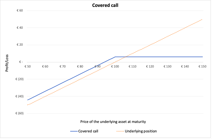
A call option gives the buyer of the option, the right but not the obligation, to buy a security at a fixed date and price defined in the contract. In a covered call, the investor writes (sells) a call option on the stock he holds in his portfolio. He earns the premium by writing the call option. Investors execute this strategy when they are bullish about the stock. The maximum payoff potential from this strategy is limited but the potential downside/losses is can be quite high (although limited).

Covered call

Buying a protective put

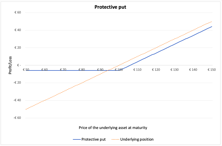
A put option gives the buyer of the option, the right but not the obligation, to sell a security at a fixed date and price defined in the contract. In a protective put, the investor buys a put option on the stock she holds in her portfolio. She pays the premium by buying the put option. Investors execute this strategy when they are bearish about the stock. The maximum payoff potential from this strategy is unlimited but the potential downside/losses is limited.

Protective Put

Spreads

Spreads are option hedging strategies where the investor/trader will take positions in multiple options of the same type (either call options or put options on the same underlying). The different types of spreads are mentioned below:

Strangle and Straddle

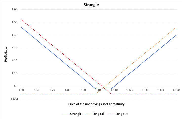
In a strangle, the investor buys a European call and a European put option, both at the same expiration date but different strike prices. To benefit from this strategy, the price of the underlying asset must move further away from the central value in either direction i.e., increase or decrease. If the stock prices stay at a level closer to the central value, the investor will incur losses. This strategy is suitable for investors who expect a huge price movement but are unsure of the direction of the movement.

Strangle

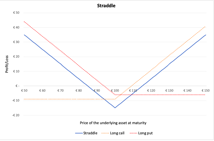
In a straddle, the investor buys a European call and a European put option, both at the same expiration date and at the same strike price. This strategy works in a similar manner like a strangle. However, the potential losses are a bit higher than incurred in a strangle if the stock price remains near the central value at expiration date.

Straddle

Bull and Bear spreads

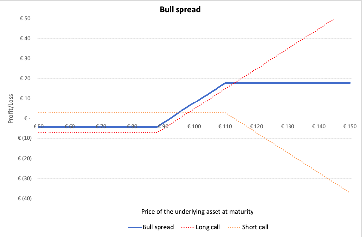
In a bull spread, the investor buys a European call option on a stock with strike price K1 and sells a call option on the same stock at strike price K2 (which is higher than K1) at the same expiration date. The investor forecasts the prices to go up and is bullish about the stock. The spread limits the potential downside risk on buying the call option, but also limits the potential profit by capping the upside. It Is used as an effective hedge to limit the losses.

Bull spread

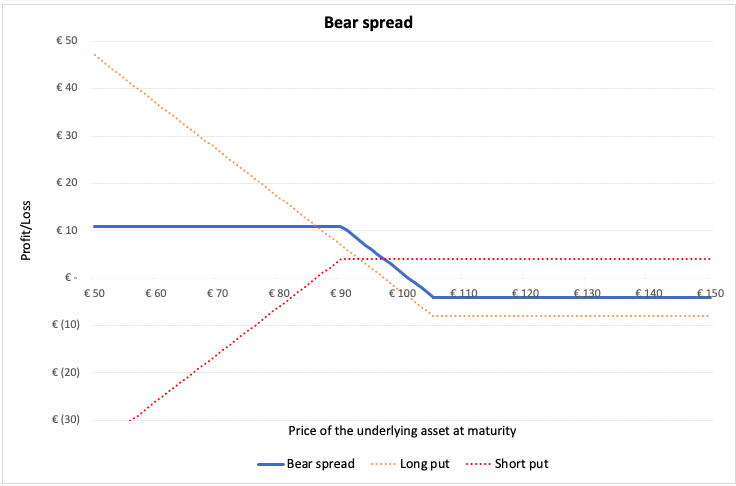
In a bear spread, the investor expects the prices of the stock to decline. In order to hedge against the downside, the investor buys a put option at strike price K2 and sells a put option at strike price K1, where K1 < K2. Initially, this strategy leads to a cash outflow since the put option is sold at a lower strike price, which results in lower premium.

Bear spread

Useful Resources

Hull J.C. (2015) Options, Futures, and Other Derivatives, Ninth Edition, Chapter 10 – Trading strategies involving Options, 276-295.

Investopedia Using Options as a Hedging Strategy

▶ Gupta A. Option Greeks – Delta

▶ Gupta A. History of Options markets

▶ Gupta A. Option Trader – Job description

▶ Gupta A. Options

About the author

Article written in September 2021 by Akshit GUPTA (ESSEC Business School, Master in Management, 2019-2022).

Types of exercise for option contracts

February 5, 2024September 19, 2021 by Akshit GUPTA

Types of exercise for option contracts

This article written by Akshit GUPTA (ESSEC Business School, Grande Ecole Program – Master in Management, 2019-2022) presents the different types of exercise for option contracts.

Introduction

Exercising a call option contract means the purchase of the underlying asset by the call buyer at the price set in the option contract (strike price). Similarly, exercising a put option contract means the sale of the underlying asset by the put buyer at the price set in the option contract.

The different option contracts can be settled in cash or with a physical delivery of the underlying asset. Normally, the equity, fixed interest security and commodity option contracts are settled using physical delivery and index options are settled in cash.

Majority of options are not exercised before the maturity date because it is not optimal for the option holder to do so. Note that for options with physical delivery, it may be better to close the position before the expiration date). If an option expires unexercised, the option holder loses any of the rights granted in the contract (indeed, in-the-money options are automatically exercised at maturity). Exercising options is a sophisticated and at times a complicated process and option holder need to take several factors into consideration while making the decision about exercise such as opinion about future market behavior of underlying asset in option, tax implications of exercise, net profit that will be acquired after deducting exercise commissions, option type, vested shares, etc.

Different types of exercise for option contracts

The option style does not deal with the geographical location of where they are traded! The contracts differ in terms of their expiration time when they can be exercised. The option contracts can be categorized as per different styles they come in. Some of the most common styles of option contracts are:

American options

American-style options give the option buyer the right to exercise his/her option anytime prior or up to the expiration date of the contract. These options provide greater flexibility to the option buyer but also come at a higher price as compared to the European-style options.

European options

European-style options can only be exercised on the expiration or maturity date of the contract. Thus, they offer less flexibility to the option buyer. However, the European options are cheaper as compared to the American options.

Bermuda options

Bermuda options are a mix of both American and European style options. These options can only be exercised on specific predetermined dates or periods up to the expiration date. They are considered to be exotic option contracts and provide limited flexibility to the option buyer.

Early Exercise

Early exercise is a strategy of exercising options before the expiration date and is possible with American options only. The question is: when the holder of an American option should exercise his/her option? Before the expiration date or at the expiration date? Quantitative models say that it could be optimal to exercise American options before the date of a dividend payout (options are not protected against the payement of dividends by firms) and sometimes for deep in-the-money put options.

There are many strategies that investors follow while exercising option contracts in order to maximize their gains and hedge risks. A few of them are discussed below:

Exercise-and-Hold

Investors can purchase their option shares with cash and hold onto them. This allows them to benefit from ownership in company stock, providing potential gains from any increase in stock value and dividend payments if any. Investors are also liable to pay brokerage commissions fees and taxes.

Exercise-and-Sell

This is a cashless strategy wherein investors purchase the option shares and then immediately sell them. Brokerages generally allow this kind of transaction without use of cash, with the money from the stock sale covering the purchase price, as well as the commissions and taxes associated with the transaction. This choice provides investors with available cash in pocket to invest elsewhere too.

Exercise-and-Sell-to-Cover

In this strategy too, investors exercise the option and then immediately sell enough shares to cover the purchase price, commissions fees and taxes. The remaining shares remain with the investor.

Useful Resources

Academic research

Hull J.C. (2015) Options, Futures, and Other Derivatives, Ninth Edition, Chapter 10 – Mechanics of options markets, 235-240.

Business analysis

Fidelity Exercising Stock Options

About the author

Article written in August 2021 by Akshit GUPTA (ESSEC Business School, Grande Ecole Program – Master in Management, 2019-2022).

Mon expérience lors de la fusion Lafarge Holcim

September 16, 2021 by Oliver BEGUE

Mon expérience lors de la fusion Lafarge Holcim

In this article, Oliver BEGUE (ESSEC Executive Education, Mastère Spécialisé Direction Financière Contrôle, 2020-2021) nous partage son expérience professionnelle lors de la fusion d’entreprises Lafarge Holcim en avril 2014.

La fusion Lafarge Holcim

Lafarge

En 2015 Lafarge était une entreprise française devenue numéro 1 mondial dans la production de ciment, béton et granulats dans le secteur du BTP avec un chiffre d’affaires de 12,8 Mds d’euros. Lafarge était côté à Euronext et faisait partie de l’indice CAC 40 avec une capitalisation boursière de 16,7 Mds d’euros.

Holcim

En 2015 Holcim est une entreprise suisse devenue numéro 2 mondial du même secteur d’activité que Lafarge (BTP) avec un chiffre d’affaires converti en euros de 19,9 Mds d’euros. Holcim était coté à la Bourse suisse (Swiss EBS Stocks) avec une capitalisation boursière convertie en euro de 21,5 Mds d’euros.

L’opération de fusion des deux entreprises

Le 5 septembre 2015, les deux groupes, Lafarges et Holcim, ont annoncé leur projet de fusion d’égal à égal (1 action Holcim pour 1 action Lafarge). Cette fusion avait deux principaux objectifs :

Générer de la trésorerie pour les actionnaires (dividendes par de meilleurs résultats)
Devenir le géant mondial du BTP pour concurrencer les entreprises fabriquant à bas couts des pays émergents.

Bilan de la fusion

L’opération de fusion a coûté plus de 2 Mds d’euros au Groupe soit le double du budget prévu. La Commission européenne, afin de valider la fusion des deux géants du BTP, a demandé la cession d’un périmètre de sociétés rentables des deux Groupes afin de maintenir la politique de concurrence de l’Union Européenne.

La fusion elle-même, et le volume d’entités cédées ont ainsi fait la une des journaux en 2015 et 2016 soulevant nombre de scandales (financement du terrorisme, obtention de l’appel d’offre du mur entre le Mexique et les Etats-Unis, présence non officielle en Iran…)
Depuis la fusion et suite à ces différents évènements, le Groupe a connu un désengagement de ses clients ayant pour conséquence la chute de son chiffre d’affaires qui atteint en 2019 24,6 Mds d’euros avec une capitalisation boursière de 27,2 Mds d’euros.

Le Groupe LafargeHolcim, en crise de croissance, rattrapé par la concurrence et les nouveaux marchés plus porteurs, et subissant le désintérêt sur le marché (chute du volume d’échanges) quitte ainsi le CAC 40 en juin 2018.

Mon expérience personnelle

La fusion Lafarge Holcim est un réel succès dans ma carrière professionnelle. En plus du volume de données à traiter étant donné la taille du groupe, les spécificités de chacun (groupe français intégré par un groupe suisse-allemand, deux outils de consolidation différents, un traitement normatif et une communication différence, une gestion RH différente), le réel challenge chez Lafarge Holcim était pour moi une question de légitimité. A à peine 24 ans, j’étais amené à valider des transactions, mais surtout à former des équipes (des centaines de personnes) aux nouveaux outils de consolidation. Former des équipes ayant mon âge en nombre d’année d’expérience fut compliqué. J’ai dû prouver mes compétences techniques et faire preuve d’empathie dans un contexte humain difficile afin de gagner la confiance de mes interlocuteurs.

Cette fusion a bel et bien été un tremplin dans ma carrière professionnelle. Néanmoins, je doute qu’elle ait été positive pour le Groupe.

Fusion d’entreprises : création de valeur ?

La fusion d’entreprises présentent des avantage set des inconvénients que nous listons ci-dessous :

Avantage :

A cout terme, la fusion Lafarge Holcim a bénéfié d’une réduction des couts fixes liés aux synergies (fermeture totale du siège social de Lafarge notamment), pour un total de 1,4 Mds d’euros. La fusion de ces deux Groupes permet aussi, dans un secteur où les ressources employées en investissements sont particulièrement important, à mutualiser les ressources et le réseau géographique en termes de périmètre de société du nouveau Groupe. Ainsi Le groupe accroîtrait sa solidité financière avec une forte génération de cash-flow et un bilan robuste.

Les implantations des deux entreprises sont complémentaires, Lafarge apportant une forte présence en Afrique et au Moyen-Orient ; Holcim, des positions majeures en Amérique latine et en Asie pacifique. La réunion de ces deux portefeuilles permettra au nouveau Groupe de disposer d’une présence géographique équilibrée dans 90 pays, dont 73 pays émergents.

Inconvénients :

Afin d’obtenir la validation de la Commission Européenne sur la fusion, les deux Groupes se sont accordés pour procéder à la cession d’un parc important d’actifs, principalement des filiales en croissance pour un total d’environ 6,5 Mds d’euros.

Aussi les synergies espérées ne représentent au total que 3,5% de la capitalisation du nouvel ensemble, ce qui est peu et ne sera pas suffisant pour combler les pertes liées au Chiffre d’affaires (scandales) et au besoin en financement toujours grandissant.

L’objectif de la fusion était de créer un géant du BTP leader incontesté du marché. Le résultat est un Groupe de taille moyenne, déficitaire, et qui tente de se désendetter en cédant toujours plus de filiales.

Ressources utiles

Rapport annuel 2014 de Lafarge

Rapport annuel 2015 de Lafarge Holcim

La Commission autorise l’acquisition, sous conditions, de Lafarge par Holcim

Précisions de Lafarge Holcim sur ses opérations en Syrie

A propos de l’auteur

Cet article a été écrit en septembre 2021 par Oliver BEGUE (ESSEC Executive Education, Mastère Spécialisé Direction Financière Contrôle, 2020-2021).

VIX index

September 12, 2021 by Youssef LOURAOUI

VIX index

In this article, Youssef LOURAOUI (ESSEC Business School, Global Bachelor of Business Administration, 2017-2021) presents the VIX index, which is a financial index that measures the uncertainty in the US equity market.

This article is structured as follows: we begin by defining the grounding notions of the VIX index. We then explain the behavior of this index and its statistical characteristics. We finish by presenting its practical usage in financial markets.

Definition

The CBOE Volatility Index, abbreviated “VIX”, is a measure of the expected S&P 500 index movement calculated by the Chicago Board Options Exchange (CBOE) from the current trading prices of options written on the S&P 500 index.

Known as Wall Street’s “fear index”, the VIX is closely monitored by a broad range of market players, and its level and pattern have become ingrained in market discussion.

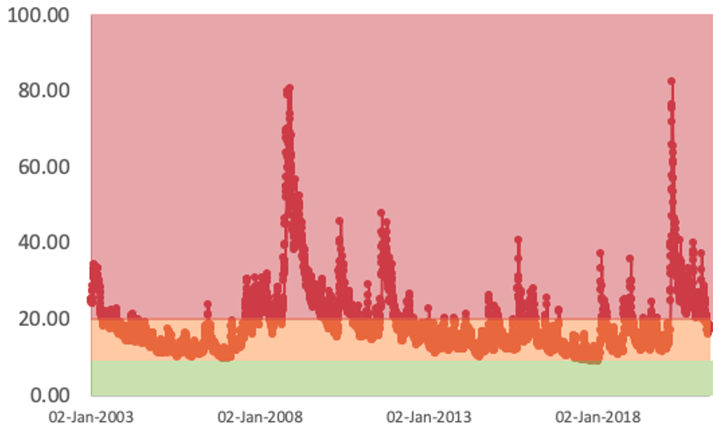
Figure 1 illustrates the evolution of the VIX index for the period from 2003 to 2021.
Figure 1 Historical levels of the VIX index from 2003-2021.

Source: computation by the author (Data source: Thomson Reuters).

VIX values greater than 20 are regarded to be high by market participants. If the VIX is between 12 and 20, it is considered normal; if it is less than 12, it is considered low. As it is the case with other indices, the VIX is computed using the price of a basket of tradable components (in this case, options expiring within the next month or so). The profit or loss that option buyers and sellers realize during the option’s life will depend, among other things, on how significantly the S&P 500’s actual volatility will differ from the implied volatility given by the VIX at the start of the period (S&P Global Research, 2017).

Behavior of the VIX index

Statistical distribution of the S&P500 index returns and VIX level

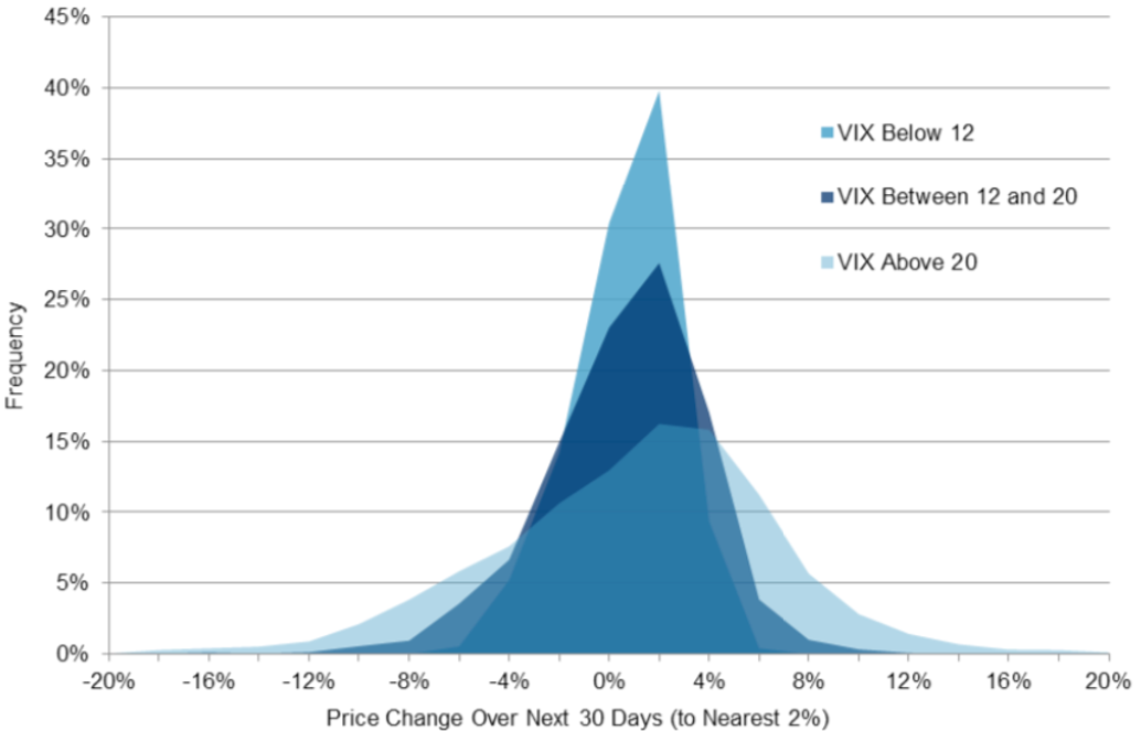
Figure 2 displays the statistical distribution of the price variations in the S&P500 index for different levels of the VIX index The higher the VIX index (by convention, greater than 20), the more severe the distribution tends to be, with negative skewness and high kurtosis indicating heightened volatility in the US market, therefore exacerbating both positive and negative swings. An opposite finding may be made for the VIX level at lower levels (often less than 12), when market swings are less evident due to less skewness and lower kurtosis (S&P Global Research, 2017).

Figure 2. The distribution of 30-day return in the S&P500 index for different VIX index levels.

Source: S&P Global Research (2017).

If the VIX is low, market players may benefit by purchasing options; conversely, if the VIX is high, market participants may profit from selling options. The specific utility of anticipated VIX is that it gives us with a more accurate assessment of whether VIX is high, low, or normal at any point in time (S&P Global Research, 2017). Thus, VIX may be regarded of as a crowd-sourced estimate of the S&P 500’s expected volatility. As with interest rates and dividends, one cannot invest directly in them, even though one can guess on their future worth, one cannot invest directly in VIX, and the significance of a specific VIX level is commonly misinterpreted (S&P Global Research, 2017).

Recent volatility in the S&P500 index and VIX level

Figure 3 demonstrates that the VIX index is strongly correlated with recent market volatility. However, there is considerable variance; for example, a recent volatility level of about 20% has been associated with a VIX level of 34 (point B, when VIX was very “high”) and with a VIX level of 12 (point C, when VIX was relatively “low”). Volatility (realized or implied) has a strong propensity to return to its mean. This insight is not especially original, despite its illustrious past. There is an enormous body of data demonstrating that volatility tends to mean revert across markets, and the pioneers of this field were given the Nobel Prize in part for incorporating their results into volatility forecasts and simulations (S&P Global Research, 2017).

Figure 3. Relation between VIX and recent volatility.

Source: S&P Global Research (2017).

Realized volatility in the S&P500 index and VIX level

Figure 4 represents the relationship between Realized volatility in the S&P500 index over a period and the VIX level at the begining of the period.

Figure 4. VIX versus next realized volatility.

Source: S&P Global Research (2017).

Mean reversion

Figure 5 shows how VIX index converge to a certain llong-term level as time passes. This finding is not due to 15% being exceptional in any manner; this figure for M was calculated using historical volatility levels for the S&P 500 and their evolution. It is not implausible that M (else referred to as long-term average volatility in the US equities market) may change over time; changes in the S&P 500’s sector weightings, trade All of these factors have the ability to influence both the pace and the volume and the point at which mean reversion occurs.

Figure 5. Mean-reversion dynamic in recent volatility.

Source: S&P Global Research (2017).

Use of the VIX index in financial markets

There are two methods for determining an asset’s volatility. Either through a statistical calculation of an asset’s realized volatility, also known as historical volatility, which serves as a pointer to the asset’s volatility behavior. This is a limited method that is based on the premise that past volatility tends to replicate itself in the future, without including a forward-looking study of volatility. The second technique is to extract an asset’s volatility from option prices referred to as “implied volatility”.

Why should I be interested in this post?

When investors make investment decisions, they utilize the VIX to gauge the degree of risk, worry, or stress in the market. Additionally, traders can trade the VIX using a range of options and exchange-traded products, or price derivatives using VIX values.

Useful resources

Business analysis

CBOE , 2021. VIX

Nasdaq, 2021. Realized Volatility

Nasdaq, 2021. Vix Index Volatility

S&P Global Research, 2017. Reading VIX: Does VIX Predict Future Volatility?

S&P Global Research, 2017. A Practitioner’s Guide to Reading VIX

About the author

The article was written in September 2021 by Youssef LOURAOUI (ESSEC Business School, Global Bachelor of Business Administration, 2017-2021).

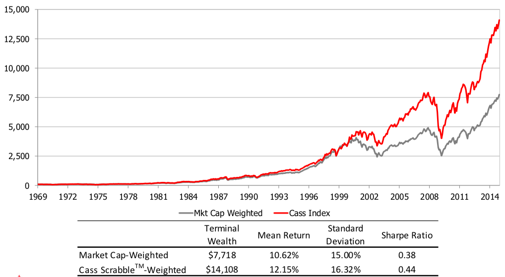
Factor Investing

September 12, 2021 by Youssef LOURAOUI

Factor Investing

In this article, Youssef LOURAOUI (ESSEC Business School, Global Bachelor of Business Administration, 2017-2021) presents factor investing, which is an investment approach that focuses on distinct performance drivers across asset classes.

This article is structured as follows: we begin with the early works of factor investing (market factor). We then delve more in detail on the different factors available and their characteristics. We finish with an empirical analysis that aims to capture the performance of factor investing across time.

Early works

In the world of investing, a factor is a persistent driver that helps explain assets’ long-term risk and return properties across asset classes. It is important to understand how factors work to better capture their potential for excess return and reduced risk across asset classes.

As a result of Harry Markowitz’s prior studies, William Sharpe, John Lintner, and Jan Mossin independently developed the Capital Asset Pricing Model (CAPM). The CAPM was a significant evolutionary step forward in capital market equilibrium theory because it allowed investors to value assets correctly in terms of systematic risk that impact all assets (Mangram, 2013). In the CAPM, the factor is the market factor representing the global uncertainty of the market.

In the late 1970s, the portfolio management industry aimed to capture the market portfolio return, but as financial research advanced and certain significant contributions were made, this gave rise to other factor characteristics to capture some additional performance.

Factor investing

As defined by Blackrock (2021), “Factor investing” is an investment strategy that focuses on unique determinants of performance across asset classes. Factor investing may improve portfolio performance and decrease volatility by increasing portfolio diversification. Asset returns are driven by two main types of factors: macroeconomic factors and style factors. Macroeconomic factors capture broad risks across asset classes while style factors explain returns and risk within asset classes.

Considering macroeconomic factors, returns can be influenced by the following macroeconomic variables (BlackRock research, 2021):

Economic growth: exposure to business and market cycles
Real interest rates: sensitivity to interest rate movements
Inflation: exposure to change in price
Credit: default risk from lending to companies
Emerging markets: political and sovereign risk
Liquidity: holding liquid assets.

Considering style factors, returns can be influenced by the following style variables (BlackRock research, 2021):

Value: stocks discounted to relative value
Minimum volatility: stable, lower risk stocks
Momentum: stocks with upward price trends
Quality: financially healthy companies
Size: smaller, high growth companies
Growth: companies that have a rate of growth above the market growth
Yield: companies that have undervalued and stable dividends

Characteristics of a factor

As defined in the work of Ang (2013) a factor must comply with the following characteristics:

A factor must be backed up by scholarly research: factors should have an academic basis. The research should illustrate either compelling logical reasoning or compelling behavioral biases, or both, in order to adequately justify the risk premium (Ang, 2013). Value, momentum, and minimum volatility among other strategies qualify as adequate risk factors under this criterion. New research may find new factors, qualify prior agreement on recognized factors, or even reject factors previously identified, all of which may be used to shape investment strategy.
A factor must have maintained a substantial risk premium in the past and is anticipated to do so in the future: not only should investors understand why the risk premium existed in the past, but they should also have some reason to believe that it will continue to exist in the future (at least in the short run). By definition, factors are systematic–they emerge from risk or behavioral patterns that will likely continue (again, in the short run), even if everyone is aware of the factors and many investors pursue the same factor strategies (no crowding effect).
A factor must be capable of being implemented in liquid, tradable instruments: factor strategies should be very inexpensive, which is best done via the use of liquid securities.

Academic literature on factor investing

Numerous academic studies and years of investing experience have revealed some types of stock, debt, and derivative assets with larger payoffs than the broad market index. Over extended periods of time, equities with low price-to-book ratios (value stocks) outperform those with high price-to-book ratios (growth stocks), creating a value-growth premium (Ang, 2013). Over time, equities with a history of high or positive returns (winners) outperform those with a history of low or negative returns (losers). This is at the heart of momentum strategies, which seeks to get exposure to stocks that have a winning tendency in the upside and downside assuming that they will continue to do well in the short term (Ang, 2013).

Investors seeking downside protection in a turbulent market environment may increase exposure to low volatility strategies, while those comfortable with more risk may choose for higher-return strategies such as momentum. The financial literature has explored deeper to show that some factors have had a long-term impact on returns. These factors contributed to returns for three reasons: an investor’s desire to take on risk, structural obstacles, and the reality that not all investors are not always entirely rational (BlackRock research, 2021). Particular factors yield higher returns as a result of increased risk but may underperform in certain market conditions. Enhanced methods use factors in more sophisticated ways, such as trading across various asset classes and sometimes investing in both long and short positions. These improved factor strategies are used by investors seeking absolute returns or as a supplement to hedge funds and classic active strategies (BlackRock research, 2021).

Securities that are less liquid trade at a discount to their more liquid counterparts and earn a higher average excess return on average. As a result, a premium is charged for illiquidity (Ang, 2013). Bonds with a greater risk of default often have higher average returns, owing to the credit risk premium. Additionally, because investors are ready to pay for protection against periods of extreme volatility, when returns tend to fall, sellers of volatility protection in option markets receive a high rate of return on average (Ang, 2013). As a result, investors can collect the premiums as follows (Ang, 2013):

The value-growth premium is equal to the difference between value and growth stocks.
The momentum premium is equal to the difference between winning and losing stocks.
The illiquidity premium is equal to the difference between the value of illiquid assets and the value of liquid assets.
The credit risk premium is the difference between the return on risky and safe debt.

These are dynamic factors, since they reflect time-varying holdings in securities that fluctuate in value over time. While dynamic factors frequently outperform the market over extended periods of time, they can significantly underperform at select occasions — such as the 2008-2009 financial crisis. While dynamic factors frequently outperform the market over extended periods of time, they can outperform the market significantly at select moments — such as the 2008-2009 financial crisis. In the long term, factor risk premiums exist to compensate investors for experiencing losses during difficult times (Ang, 2013). In the end, the factors are not ideal for everyone due to the inherent risk associated with factor techniques.

Empirical analysis

Hodges et al. (2017) published a study in the Journal of Portfolio Management that looks at the performance of factor funds over a 30-year period and examines the vectors of returns). Figure 1 illustrates the average excess returns (above the MSCI USA Index) of each factor from June 30, 1988 to September 30, 2016. Value, quality, momentum, and size all have positive average returns; momentum and value have the largest annual excess returns of 3.4 percent and 1.5 percent, respectively. Minimum volatility has generated an average return comparable to the market (but with less risk), similar with Ang’s findings (Hodges et al., 2017).

Figure 1. Factor analysis from 1988 – 2016. Average excess return.

Source: Hodges et al. (2017).

Figure 2 plots 12-month moving averages of excess factor returns and demonstrates that, while longrun excess premiums are positive, there is significant temporal variation throughout the sample. For instance, size changes from a negative 12-month mean return of -2.0 percent in 1999 to a positive 12-month mean return of 3.0 percent in the early 2000s.

Figure 2. Smart beta excess returns for the period from 1988 to 2016.

Source: Hodges et al. (2017).

Figure 3 demonstrates that the excess factor returns are not substantially correlated: the lowest correlation is -0.42, while the largest is 0.67, between minimal volatility and size. Notably, momentum and value are negatively connected with a correlation coefficient of -0.22, which is consistent with their well-known negative association (Hodges, et al., 2017).

Figure 3. Correlation analysis of smart beta excess returns for the period from 1988 to 2016.

Source: Hodges et al. (2017).

Why should I be interested in this post?

Numerous equity investors seeking greater returns at a cheaper cost have shifted their focus to factor investing. Active managers in the traditional sense typically make investing decisions based on their research of particular companies and their stocks. By contrast, factor strategies identify the qualities, or factors, that are most likely to beat the market and then invest in stocks that exhibit those characteristics. For instance, the value factor is based on the strategy of investing in companies that are undervalued in comparison to the market, whereas the momentum factor is based in the strategy of investing in equities that have recently seen a price acceleration.

Useful resources

Academic research

Ang, A., 2013. Factor Investing. Working paper.

Hodges, P., Hogan, K., Peterson, J. R., Ang, A., 2017. Factor Timing with Cross- Sectional and Time-Series Predictors. The Journal of Portfolio Management 44(1): 30-43.

Business Analysis

BlackRock research, 2021. What is Factor Investing?

About the author

The article was written in September 2021 by Youssef LOURAOUI (ESSEC Business School, Global Bachelor of Business Administration, 2017-2021).

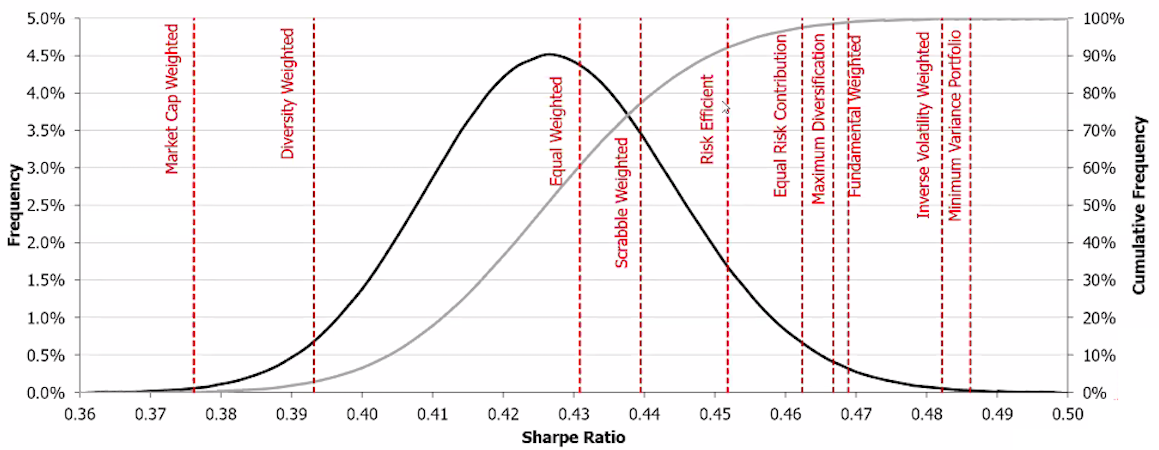
Origin of factor investing

September 12, 2021 by Youssef LOURAOUI

Origin of factor investing

In this article, Youssef LOURAOUI (ESSEC Business School, Global Bachelor of Business Administration, 2017-2021) presents the origin of factor investing. A factor is defined as a persistent driver that helps explain assets’ long-term risk and return properties across asset classes.

This article is structured as follows: we begin by presenting Markowitz’s Modern Portfolio Theory (MPT) as the origin of factor investing (market factor). We then explain the Fama-French three-factor models, which is an extension of the CAPM single factor model (market factor). Furthermore, we explain also the Carhart four-factor model and the Fama-French five-factor model that aimed to capture additional factors to the market factor.

Markowitz’s Modern Portfolio Theory: Origin of the factor investing

Factor investing can be retraced to the work of Harry Markowitz in the early 1950s. The most important aspect of Markowitz’s approach was his fundamental finding that an asset’s risk and return should not be evaluated on its own, but rather on how it contributes to the entire risk and return of a portfolio. His dissertation, titled “Portfolio Selection”, was published in The Journal of Finance (1952). Nearly thirty years later, Markowitz shared the Nobel Prize for economics and corporate finance for his MPT contributions to both disciplines. The holy grail of Markowitz’s work is based on his calculation of the variance of a two-asset portfolio computed as follows:

Where:

w and (1-w) represents asset weights of assets A and B
σ² represents the variance of the assets and portfolio
cov(r_A,r_B) represents the covariance of assets A and B.

Capital Asset Pricing Model (CAPM)

William Sharpe, John Lintner, and Jan Mossin separately developed another key capital markets theory as a result of Markowitz’s previous works : the Capital Asset Pricing Model (CAPM). The CAPM was a huge evolutionary step forward in capital market equilibrium theory, since it enabled investors to appropriately value assets in terms of systematic risk, defined as the market risk which cannot be neutralized by the effect of diversification. In his derivation of the CAPM, Sharpe, Mossin and Litner made significant contributions to the concepts of the Efficient Frontier and Capital Market Line. Sharpe, Litner and Mossin seminal contributions would later earn him the Nobel Prize in Economics. The CAPM is based on a set of market structure and investor hypotheses:

There are no intermediaries
There are no limits (short selling is possible)
Supply and demand are in balance
There are no transaction costs
An investor’s portfolio value is maximized by maximizing the mean associated with projected returns while reducing risk variance
Investors have simultaneous access to information in order to implement their investment plans
Investors are seen as “rational” and “risk averse”.

Under this framework, the expected return of a given asset is related to its risk measured by the beta:

Where :

E(r) represents the expected return of the asset
r_f the risk-free rate
β a measure of the risk of the asset
E(r_m) the expected return of the market
E[r_m– r_f]represents the market risk premium.

In this model, the beta (β) parameter is a key parameter and is defined as:

Where:

Cov(r, r_m) represents the covariance of the asset with the market
σ²(r_m) is the variance of market return.

The beta is a measure of how sensitive an asset is to market swings. This risk indicator aids investors in predicting the fluctuations of their asset in relation to the wider market. It compares the volatility of an asset to the systematic risk that exists in the market. The beta is a statistical term that denotes the slope of a line formed by a regression of data points comparing stock returns to market returns. It aids investors in understanding how the asset moves in relation to the market. According to Fama and French (2004), there are two ways to interpret the beta employed in the CAPM:

According to the CAPM formula, beta may be thought in mathematical terms as the slope of the regression between the asset return and the market return. Thus, beta quantifies the asset sensitivity to changes in the market return;
According to the beta formula, it may be understood as the risk that each dollar invested in an asset adds to the market portfolio. This is an economic explanation based on the observation that the market portfolio’s risk (measured by 〖σ(r_m)〗^2) is a weighted average of the covariance risks associated with the assets in the market portfolio, making beta a measure of the covariance risk associated with an asset in comparison to the variance of the market return.

Additionally, the CAPM makes a distinction between two forms of risk: systematic and specific risk. Systematic risk refers to the risk posed by the market’s basic structure, its participants, and any and all non-diversifiable elements such as monetary policy, political events, and natural disasters. By contrast, specific risk refers to the risk inherent in a particular asset and so is diversifiable. As a result, the CAPM solely captures systematic risk via the beta measure, with the market’s beta equal to one, lower-risk assets having a beta less than one, and higher-risk assets having a beta larger than one.

Finally, the CAPM’s central message is that when investors invest in a particular security/portfolio, they are rewarded twice: once via the time value of money impact (reflected in the risk-free component of the CAPM equation) and once via the effect of taking on more risk. However, the CAPM is not an empirically sound model, owing to an unnecessarily simplified set of assumptions and problems in establishing validating tests at the model’s first introduction (Fama and French, 2004). Thus, throughout time, the CAPM has been revised and modified to address not just its inadequacies but also to keep pace with financial and economic changes. Sharpe (1990), in his evaluation of the CAPM, cites various examples of revisions to his basic model proposed by other economists and financial experts.

The Fama-French three-factor model

Eugene Fama and Kenneth French created the Fama-French Three-Factor model in 1993 in response to the CAPM’s inadequacy. It contends that, in addition to the market risk component introduced by the CAPM, two more factors affect the returns on securities and portfolios: market capitalization (referred to as the “size” factor) and the book-to-market ratio (referred to as the “value” factor). According to Fama and French, the primary rationale for include these characteristics is because both size and book-to-market (BtM) ratios are related to the economic fundamentals of the business issuing the securities (Fama and French, 1993).

They continue by stating that:

Earnings and book-to-market ratios are inversely associated, with companies with low book-to-market ratios consistently reporting better earnings than those with high book-to-market ratios
Due to a similar risk component, size and average returns are inversely associated. This is based on their observation of the trajectory of small business profits in the 1980s: they suggest that small enterprises experience longer durations of earnings depression than larger enterprises in the event of a recession in the economy in which they operate. Additionally, they noted that smaller enterprises did not contribute to the economic expansion in the mid- and late-1980s following the 1982 recession
Profitability is connected to both size and BtM, and is a common risk factor that emphasizes and explains the positive association between BtM ratios and average returns. As thus, the return on a security/portfolio becomes:

Where :

E(𝑟) is the expected return of the asset/portfolio
𝑟_𝑓 is the risk-free rate
𝛽 is the measure of the market risk of the asset
𝐸(𝑟_𝑀) is the expected return of the market
𝛽_𝑆 is the measure of the risk related to the size of the asset
𝛽_𝑉 is the measure of the risk related to the value of the security/portfolio
𝑆𝑀𝐵 (which stands for “Small Minus Big”) measures the difference in expected returns between small and big firms (in terms of market capitalization)
𝐻𝑀𝐿 (which stands for “High Minus Low”) measures the difference in expected returns between value stocks and growth stock
𝛼 is a regression intercept
𝜖 is a measure of regression error

Both SMB and HML are derived using historical data as well as a mixture of portfolios focused on size and value. Professor French publishes these values on a regular basis on his personal website. Meanwhile, the betas for both the size and value components are derived using linear regression and might be positive or negative. However, the Fama-French three-factor model is not without flaws. Griffin (2002) highlights a significant flaw in the model when he claims that the Fama-French components of value and size are more accurate at explaining return differences when applied locally rather than internationally. As a result, each of the components should be addressed on a nation-by-country basis (as professor French now does on his website, where he specifies the SMB and HML factors for each nation, such as the United Kingdom, France, and so on). While the Fama-French model has gone further than the CAPM in terms of breaking down security returns, it remains an incomplete model with spatially confined interpretation of its additional variables. Efforts have been made over the years to complete this model, with Fama and French adding two more variables in 2015, profitability and investment strategy, and other scholars, like as Carhart (1997), adding a fourth feature, momentum, to the original Three-Factor model.

The Carhart four-factor model

Carhart (1997) extended the Fama-French three-factor model (1993) by adding a fourth factor: momentum. Momentum is defined as the observable tendency for prices to continue climbing or declining following an initial increase or decline. By definition, momentum is an anomaly, as the Efficient Market Hypothesis (EMH) states that there is no reason for security prices to continue growing or declining after an initial change in their value.

While traditional financial theory is unable to define precisely what causes momentum in certain securities, behavioural finance provides some insight into why momentum exists; indeed, Chan, Jegadeesh and Lakonishok (1996) argue that momentum arises from the inability of the majority of investors to react quickly and immediately to new market information and, thus, integrate that information into securities. This argument demonstrates investors’ irrationality when it comes to appraising the value of certain stocks and making investing decisions. Carhart was motivated to incorporate the momentum component into the Fama-French three-factor model since the model was unable to account for return variance in momentum-sorted portfolios (Fama and French, 1996 – Carhart 1997). Carhart incorporated Jegadeesh and Titman’s (1993) one-year momentum variation into his model as a result.

Where the additional component represents:

𝛽_𝑀 is the measure of the risk related to the momentum factor of the security/portfolio
𝑈𝑀𝐷 (which stands for “Up Minus Down”) measures the difference in expected returns between “winning” securities and “losing” securities (in terms of momentum).

As Carhart states in his article, the four-factor model, like the CAPM and the Fama-French Three-Factor, may be used to explain the sources of return on a specific security/portfolio (Carhart, 1997).

The Fama-French five-factor model

Fama and French state in 2014 that the first three-factor model they developed in 1993 does not adequately account for certain observed inconsistencies in predicted returns. As a consequence, Fama and French enhanced the three-factor model by adding two new variables: profitability and investment. The justification for these two factors arises from the theoretical implications of the dividend discount model (DDM), which claims that profitability and investment help to explain the returns achieved from the HML element in the first model (Fama and French, 2015).

Surprisingly, unlike the Carhart model, the new Fama-French model does not incorporate the momentum element. This is mostly because to Fama’s position on momentum. While not denying its existence, Fama thinks that the degree of risk borne by securities in an efficient market cannot fluctuate so dramatically that it justifies the necessity to recognize the momentum factor’s involvement (Fama and French, 2015). According to the Fama-French five-factor model, the return on any security is calculated as follows:

𝛽_P is the measure of the risk related to the profitability factor of the security/portfolio
𝑅𝑀𝑊 (which stands for “Robust Minus Weak”) measures the difference in expected returns between securities that exhibit strong profitability levels (thus making them “robust”) and securities that show inconsistent profitability levels (thus making them “weak”)
𝛽_𝐼 is the measure of the risk related to the investment factor of the asset
𝐶𝑀𝐴 (which stands for “Conservative Minus Aggressive”) measures the difference in expected returns between securities that engage in limited investment activities (thus making them “conservative”) and securities that show high levels of investment activity (thus making them “aggressive”).

To validate the new model, Fama and French created many portfolios with considerable returns disparities due to size, value, profitability, and investing characteristics. Additionally, they completed two exercises:

The first is a regression of portfolio results versus the improved model. This was done to determine the extent to which it explains the observed returns disparities between the selected portfolios
The second is to compare the new model’s performance to that of the three-factor model. This was done to determine if the new five-factor model adequately accounts for the observed returns differences in the old three-factor model. The following summarizes Fama and French’s conclusions about the new model.

The HML component becomes superfluous in terms of structure, since any value contribution to a security’s return can already be accounted by market, size, investment, and profitability factors. Thus, Fama and French advise investors and scholars to disregard the HML effect if their primary objective is to explain extraordinary returns (Fama and French, 2015).

They do, however, argue for the inclusion of all five elements when attempting to explain portfolio returns that display size, value, profitability, and investment tilts. Additionally, the model explains between 69% and 93% of the return disparities seen following the usage of the prior three-factor model (Fama and French, 2015). This new model, however, is not without flaws. Blitz, Hanauer, Vidojevic, and van Vliet (henceforth referred to as BHVV) identified five problems with the new Fama-French five-factor model in their 2016 paper “Five difficulties with the Five-Factor model”.

While two of these issues are related to some of the original Fama-French three factor model’s original factors (most notably the continued existence within the model of the CAPM relationship between market risk and return, as well as the new model’s overall acceptance by the academic community while some of the original factors are still contested), several of the other issues are related to other factors. These concerns include the following (Fama and French, 2015) :

The lack of motion
The new factors introduced lack robustness. The questions here include historical (i.e., will these factors apply to data points before to 1963) and if these aspects also apply to other asset types
The absence of adequate empirical support for the implementation of these Fama and French components

Use of the asset pricing models

All the models presented above are mostly employed in asset management to analyze the performance of an actively managed portfolio and the overall performance of a mutual fund.

Why should I be interested in this post?

In the CAPM, the factor is the market factor representing the global uncertainty of the market. In the late 1970s, the portfolio management industry aimed to capture the market portfolio return, but as financial research advanced and certain significant contributions were made, this gave rise to other factor characteristics to capture some additional performance. Analyzing the historical contributions that underpins factor investing is fundamental in order to have a better understanding of the subject.

Useful resources

Academic research

Blitz, D., Hanauer M.X., Vidojevic M., van Vliet, P., 2018. Five Concerns with the Five-Factor Model, The Journal of Portfolio Management, 44(4): 71-78.

Carhart, M.M. (1997), On Persistence in Mutual Fund Performance. The Journal of Finance, 52: 57-82.

Fama, E.F., French, K.R., 1992. The Cross-Section of Expected Stock Returns. The Journal of Finance, 47: 427-465.

Fama, E.F., French, K.R., 2004. The Capital Asset Pricing Model: Theory and Evidence. Journal of Economic Perspectives, 18(3): 25-46.

Fama, E.F., French, K.R., 2015. A five-factor asset pricing model. Journal of Financial Economics, 116(1): 1-22.

Lintner, J. 1965a. The Valuation of Risk Assets and the Selection of Risky Investments in Stock Portfolios and Capital Budgets. The Review of Economics and Statistics 47(1): 13-37.

Lintner, J. 1965b. Security Prices, Risk and Maximal Gains from Diversification. The Journal of Finance 20(4): 587-615.

Mangram, M.E., 2013. A simplified perspective of the Markowitz Portfolio Theory. Global Journal of Business Research, 7(1): 59-70.

Markowitz, H., 1952. Portfolio Selection. The Journal of Finance, 7(1): 77-91.

Mossin, J. 1966. Equilibrium in a Capital Asset Market. Econometrica 34(4): 768-783.

Sharpe, W.F. 1963. A Simplified Model for Portfolio Analysis. Management Science 9(2): 277-293.

Sharpe, W.F. 1964. Capital Asset Prices: A theory of Market Equilibrium under Conditions of Risk. The Journal of Finance 19(3): 425-442.

About the author

The article was written in September 2021 by Youssef LOURAOUI (ESSEC Business School, Global Bachelor of Business Administration, 2017-2021).

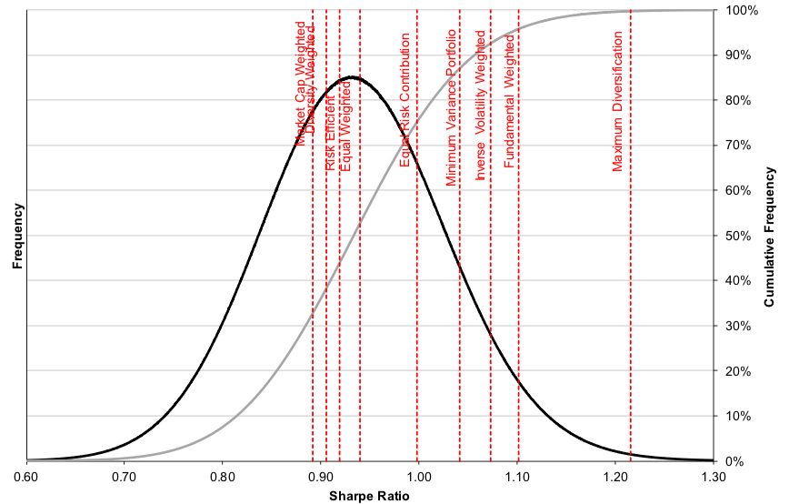
Capital Asset Pricing Model (CAPM)

September 6, 2021 by Jayati WALIA

Capital Asset Pricing Model (CAPM)

In this article, Jayati WALIA (ESSEC Business School, Grande Ecole Program – Master in Management, 2019-2022) presents the Capital Asset Pricing Model (CAPM).

Introduction

The Capital Asset Pricing Model (CAPM) is a widely used metrics for the financial analysis of the performance of stocks. It shows the relationship between the expected return and the systematic risk of investing in an asset. The idea behind the model is that the higher the risk in an investment in securities, the higher the returns an investor should expect on his/her investments.

The Capital Asset Pricing Model was developed by financial economists William Sharpe, John Lintner, Jack Treynor and Jan Mossin independently in the 1960s. The CAPM is essentially built on the concepts of the Modern Portfolio Theory (MPT), especially the mean-variance analysis model by Harry Markowitz (1952).

CAPM is very often used in the finance industry to calculate the cost of equity or expected returns from a security which is essentially the discount rate. It is an important tool to compute the Weighted Average Cost of Capital (WACC). The discount rate is then used to ascertain the Present Value (PV) and Net Present Value (NPV) of any business or financial investment.

CAPM formula

The main result of the CAPM is a simple mathematical formula that links the expected return of an asset to its risk measured by the beta of the asset:

CAPM risk beta relation

Where:

E(r_i) represents the expected return of asset i
r_f the risk-free rate
β_i the measure of the risk of asset i
E(r_m) the expected return of the market
E(r_m)- r_f the market risk premium.

The risk premium for asset i is equal to β_i(E(r_m)- r_f), that is the beta of asset i, β_i, multiplied by the risk premium for the market, E(r_m)- r_f.

The formula shows that investors demand a return higher than the risk-free rate for taking higher risk. The equity risk premium is the component that reflects the excess return investors require on their investment.

Let us discuss the components of the Capital Asset Pricing Model individually:

Expected return of the asset: E(r_i)

The expected return of the asset is essentially the minimum return that the investor should demand when investing his/her money in the asset. It can also be considered as the discount rate the investor can utilize to ascertain the value of the asset.

Risk-free interest rate: r_f

The risk-free interest rate is usually taken as the yield on debt issued by the government (the 3-month Treasury bills and the 10-year Treasury bonds in the US) as they are the safest investments. As government bonds have very rare chances of default, their interest rates are considered risk-free.

Beta: β

The beta is a measure of the systematic or the non-diversifiable risk of an asset. This essentially means the sensitivity of an asset price compared to the overall market. The market beta is equal to 1. A beta greater than 1 for an asset signifies that the asset is riskier compared to the overall market, and a beta of less than 1 signifies that the asset is less risky compared to the overall market.

The beta is calculated by using the equation:

CAPM beta formula

Where:

Cov(r_i, r_m) represents the covariance of the return of asset i with the return of the market
σ²(r_m) the variance of the return of the market.

The beta of an asset is defined as the ratio of the covariance between the asset return and the market return, and the variance of the market return.

The covariance is a measure of correlation between two random variables. In practice, the covariance is calculated using historical data for the asset return and the market return.

The variance is a measure of the dispersion of returns. The standard deviation, equal to the square root of the variance, is a measure of the volatility in the market returns over time.

Expected market return

The expected market return is usually computed using historical data of the market. The market is usually represented by a stock index to which the stock belongs to.

For example, for calculating the expected return on APPLE stock, we usually consider the S&P 500 index. Historically, the expected return for the S&P 500 index is around 9%.

Assumptions in Capital Asset Pricing Model

The CAPM considers the following assumptions which forms the basis for the model:

Investors are risk averse and rational – In the CAPM, all investors are assumed to be risk averse. They diversify their portfolio which neutralizes the non-systematic or the diversifiable risk. So, in the end only the systematic or the market risk is considered to calculate the expected returns on the security.
Efficient markets – The markets are assumed to be efficient, thus all investors have equal access to the same information. Also, all the assets are considered to be liquid, and an individual investor cannot influence the future prices of an asset.
No transaction costs – The CAPM assumes that there are no transaction costs, taxes, and restrictions on borrowing or lending activities.
Risk premium – The CAPM model assumes that investors require higher premium for more risk they take (risk aversion).

Example

As an example, lest us consider an investor who wants to calculate the expected return on an investment in APPLE stock. Let’s see how the CAPM can be used in this case.

The risk-free interest rate is taken to be the current yield on 10-year US Treasury bonds. Let us assume that its value is 3%.

The S&P 500 index has an expected return of 9%.

The beta on APPLE stock is 1.25.

The expected return on APPLE stock is equal to 3% + 1.25*(9% – 3%) = 10.50%

Useful resources

Acadedmic articles

Lintner, J. (1965) The Valuation of Risk Assets and the Selection of Risky Investments in Stock Portfolios and Capital Budgets The Review of Economics and Statistics 47(1) 13-37.

Markowitz, H. (1952) Portfolio Selection The Journal of Finance 7(1) 77-91.

Mossin, J. (1966) Equilibrium in a Capital Asset Market Econometrica 34(4) 768-783.

Merton, R.C. (1973) An Intertemporal Capital Asset Pricing Model Econometrica 41(5) 867-887.

Sharpe, W.F. (1964) Capital Asset Prices: A Theory of Market Equilibrium Under Conditions of Risk The Journal of Finance 19(3) 425-442.

Business sources

Mullins, D.W. Jr (1982) Does the Capital Asset Pricing Model Work? Harvard Business Review.

About the author

The article was written in September 2021 by Jayati WALIA (ESSEC Business School, Grande Ecole Program – Master in Management, 2019-2022).

Quantitative risk management

September 6, 2021 by Jayati WALIA

Quantitative risk management

In this article, Jayati WALIA (ESSEC Business School, Grande Ecole Program – Master in Management, 2019-2022) presents Quantitative risk management.

Introduction

Risk refers to the degree of uncertainty in the future value of an investment or the potential losses that may occur. Risk management forms an integral part of any financial institution to safeguard the investments against different risks. The key question that forms the backbone for any risk management strategy is the degree of variability in the profit and loss statement for any investment.

The process of the risk management has three major phases. The first phase is risk identification which mainly focuses on identifying the risk factors to which the institution is exposed. This is followed by risk measurement that can be based on different types of metrics, from monitoring of open positions to using statistical models and Value-at-Risk. Finally, in the third phase risk management is performed by setting risk limits based on the determined risk appetite, back testing (testing the quality of the models on the historical data) and stress testing (assessing the impact of severe but still plausible adverse scenarios).

Different types of risks

There are several types of risks inherent in any investment. They can be categorized in the following ways:

Market risk

An institution can invest in a broad list of financial products including stocks, bonds, currencies, commodities, derivatives, and interest rate swaps. Market risk essentially refers to the risk arising from the fluctuation in the market prices of these assets that an institution trades or invests in. The changes in prices of these underlying assets due to market volatility can cause financial losses and hence, to analyze and hedge against this risk, institutions must constantly monitor the performance of the assets. After measuring the risk, they must also implement necessary measures to mitigate these risks to protect the institution’s capital. Several types of market risks include interest rate risk, equity risk, currency risk, credit spread risk etc.

Credit risk

The risk of not receiving promised repayments due to the counterparty failing to meet its obligations is essentially credit risk. The counterparty risk can arise from changes in the credit rating of the issuer or the client or a default on a due obligation. The default risk can arise from non-payments on any loans offered to the institution’s clients or partners. After the financial crisis of 2008-09, the importance of measuring and mitigating credit risks has increased many folds since the crisis was mainly caused by defaults on payments on sub-prime mortgages.

Operational risk

The risk of financial losses resulting from failed or faulty internal processes, people (human error or fraud) or system, or from external events like fraud, natural calamities, terrorism etc. refers to operational risk. Operational risks are generally difficult to measure and may cause potentially high impacts that cannot be anticipated.

Liquidity risk

The liquidity risk comprises to 2 types namely, market liquidity risk and funding liquidity risk. In market liquidity risk can arise from lack of marketability of an underlying asset i.e., the assets are comparatively illiquid or difficult to sell given a low market demand. Funding liquidity risk on the other hand refers to the ease with which institutions can raise funding and thus institutions must ensure that they can raise and retain debt capital to meet the margin or collateral calls on their leveraged positions.

Strategic risk

Strategic risks can arise from a poor strategic business decisions and include legal risk, reputational risk and systematic and model risks.

Basel Committee on Banking Supervision

The Basel Committee on Banking Supervision (BCBS) was formed in 1974 by central bankers from the G10 countries. The committee is headquartered in the office of the Bank for International Settlements (BIS) in Basel, Switzerland. BCBS is the primary global standard setter for the prudential regulation of banks and provides a forum for regular cooperation on banking supervisory matters. Its 45 members comprise central banks and bank supervisors from 28 jurisdictions. Member countries include Australia, Belgium, Canada, Brazil, China, France, Hong Kong, Italy, Germany, India, Korea, the United States, the United Kingdom, Luxembourg, Japan, Russia, Switzerland, Netherlands, Singapore, South Africa among many others.

Over the years, BCBS has developed influential policy recommendations concerning international banking and financial regulations in order to exercise judicious corporate governance and risk management (especially market, credit and operational risks), known as the Basel Accords. The key function of Basel accords is to manage banks’ capital requirements and ensure they hold enough cash reserves to meet their respective financial obligations and henceforth survive in any financial and/or economic distress.

Over the years, the following versions of the Basel accords have been released in order to enhance international banking regulatory frameworks and improve the sector’s ability to manage with financial distress, improve risk management and promote transparency:

Basel I

The first of the Basel accords, Basel I (also known as Basel Capital Accord) was developed in 1988 and implemented in the G10 countries by 1992. The regulations intended to improve the stability of the financial institutions by setting minimum capital reserve requirements for international banks and provided a framework for managing of credit risk through the risk-weighting of different assets which was also used for assessing banks’ credit worthiness.
However, there were many limitations to this accord, one of which being that Basel I only focused on credit risk ignoring other risk types like market risk, operational risk, strategic risk, macroeconomic conditions etc. that were not covered by the regulations. Also, the requirements posed by the accord were nearly the same for all banks, no matter what the bank’s risk level and activity type.

Basel II

Basel II regulations were developed in 2004 as an extension of Basel I, with a more comprehensive risk management framework and thereby including standardized measures for managing credit, operational and market risks. Basel II strengthened corporate supervisory mechanisms and market transparency by developing disclosure requirements for international regulations inducing market discipline.

Basel III

After the 2008 Financial Crisis, it was perceived by the BCBS that the Basel regulations still needed to be strengthened in areas like more efficient coverage of banks’ risk exposures and quality and measure of the regulatory capital corresponding to banks’ risks.
Basel III intends to correct the miscalculations of risk that were believed to have contributed to the crisis by requiring banks to hold higher percentages of their assets in more liquid instruments and get funding through more equity than debt. Basel III thus tries to strengthen resilience and reduce the risk of system-wide financial shocks and prevent future economic credit events. The Basel III regulations were introduced in 2009 and the implementation deadline was initially set for 2015 however, due to conflicting negotiations it has been repeatedly postponed and currently set to January 1, 2022.

Risk Measures

Efficient risk measurement based on relevant risk measures is a fundamental pillar of the risk management. The following are common measures used by institutions to facilitate quantitative risk management:

Value at risk (VaR)

VaR is the most extensively used risk measure and essentially refers to the maximum loss that should not be exceeded during a specific period of time with a given probability. VaR is mainly used to calculate minimum capital requirements for institutions that are needed to fulfill their financial obligations, decide limits for asset management and allocation, calculate insurance premiums based on risk and set margin for derivatives transactions.
To estimate market risk, we model the statistical distribution of the changes in the market position. Usual models used for the task include normal distribution, the historical distribution and the distributions based on Monte Carlo simulations.

Expected Shortfall

The Expected Shortfall (ES) (also known as Conditional VaR (CVaR), Average Value at risk (AVaR), Expected Tail Loss (ETL) or Beyond the VaR (BVaR)) is a statistic measure used to quantify the market risk of a portfolio. This measure represents the expected loss when it is greater than the value of the VaR calculated with a specific probability level (also known as confidence level).

Credit Risk Measures

Probability of Default (PD) is the probability that a borrower may default on his debt over a period of 1 year. Exposure at Default (EAD) is the expected amount outstanding in case the borrower defaults and Loss given Default (LGD) refers to the amount expected to lose by the lender as a proportion of the EAD. Thus the expected loss in case of default is calculated as PD*EAD*LGD.

Useful resources

Articles

Longin F. (1996) The asymptotic distribution of extreme stock market returns Journal of Business, 63, 383-408.

Longin F. (2000) From VaR to stress testing : the extreme value approach Journal of Banking and Finance, 24, 1097-1130.

Longin F. and B. Solnik (2001) Extreme correlation of international equity markets Journal of Finance, 56, 651-678.

Books

Embrechts P., C. Klüppelberg and T Mikosch (1997) Modelling Extremal Events for Insurance and Finance.

Embrechts P., R. Frey, McNeil A. J. (2022) Quantitative Risk Management, Princeton University Press.

Gumbel, E. J. (1958) Statistics of extremes. New York: Columbia University Press.

Longin F. (2016) Extreme events in finance: a handbook of extreme value theory and its applications Wiley Editions.
Corporate Finance Institute Basel Accords

Other materials

Extreme Events in Finance

QRM Tutorial

About the author

The article was written in September 2021 by Jayati WALIA (ESSEC Business School, Grande Ecole Program – Master in Management, 2019-2022).

Brownian Motion in Finance

January 30, 2024September 6, 2021 by Jayati WALIA

Brownian Motion in Finance

In this article, Jayati WALIA (ESSEC Business School, Grande Ecole Program – Master in Management, 2019-2022) explains the Brownian motion and its applications in finance to model asset prices like stocks traded in financial markets.

Introduction

Stock price movements form a random pattern. The prices fluctuate everyday resulting from market forces like supply and demand, company valuation and earnings, and economic factors like inflation, liquidity, demographics of country and investors, political developments, etc. Market participants try to anticipate stock prices using all these factors and contribute to make price movements random by their trading activities as the financial and economics worlds are constantly changing.

What is a Brownian Motion?

The Brownian motion was first introduced by botanist Robert Brown who observed the random movement of pollen particles due to water molecules under a microscope. It was in the 1900s that the French mathematician Louis Bachelier applied the concept of Brownian motion to asset price behavior for the first time, and this led to Brownian motion becoming one of the most important fundamental of modern quantitative finance. In Bachelier’s theory, price fluctuations observed over a small time period are independent of the current price along with historical behavior of price movements. Combining his assumptions with the Central Limit Theorem, he also deduces that the random behavior of prices can be said to be represented by a normal distribution (Gaussian distribution).

This led to the development of the Random Walk Hypothesis or Random Walk Theory, as it is known today in modern finance. A random walk is a statistical phenomenon wherein stock prices move randomly.

When the time step of a random walk is made infinitesimally small, the random walk becomes a Brownian motion.

Standard Brownian Motion

In context of financial stochastic processes, the Brownian motion is also described as the Wiener Process that is a continuous stochastic process with normally distributed increments. Using the Wiener process notation, an asset price model in continuous time can be expressed as:

brownian motion equation

with dS being the change in asset price in continuous time dt. dX is the random variable from the normal distribution (N(0, 1) or Wiener process). σ is assumed to be constant and represents the price volatility considering the unexpected changes that can result from external effects. μdt together represents the deterministic return within the time interval with μ representing the growth rate of asset price or the ‘drift’.

When the market is modeled with a standard Brownian Motion, the probability distribution function of the future price is a normal distribution.

Geometric Brownian Motion

weiner notation

When the market is modeled with a geometric Brownian Motion, the probability distribution function of the future price is a log-normal distribution.

Properties of a Brownian Motion

Continuity: Brownian motion is the continuous time-limit of the discrete time random walk. It thus, has no discontinuities and is non-differential everywhere.
Finite: The time increments are scaled with the square root of the times steps such that the Brownian motion is finite and non-zero always.
Normality: Brownian motion is normally distributed with zero mean and non-zero standard deviation.
Martingale and Markov Property: Martingale property states that the conditional expectation of the future value of a stochastic process depends on the current value, given information about previous events. The Markov property instead focusses on the ‘no memory’ theory that the expected future value of a stochastic process does not depend on any past values except the current value. Brownian motion follows both these properties.

Simulating Random Walks for Stock Prices

In quantitative finance, a random walk can be simulated programmatically through coding languages. This is essential because these simulations can be used to represent potential future prices of assets and securities and work out problems like derivatives pricing and portfolio risk evaluation.

A very popular mathematical technique of doing this is through the Monte Carlo simulations. In option pricing, the Monte Carlo simulation method is used to generate multiple random walks depicting the price movements of the underlying, each with an associated simulated payoff for the option. These payoffs are discounted back to the present value and the average of these discounted values is set as the option price. Similarly, it can be used for pricing other derivatives, but the Monte Carlo simulation method is more commonly used in portfolio and risk management.

For instance, consider Microsoft stock that has a current price of $258.65 with a growth trend of 55.2% and a volatility of 35.92%.

A plot of daily returns represented as a random normal distribution is:

Normal Distribution

The above figure represents the simulated price path according to the Geometric Brownian motion for the Microsoft stock price. Similarly, a plot of 10 such simulations would be like this:

Microsoft GBM Simulations

Thus, we can see that with just 10 simulations, the prices range from $100 to over $600. We can increase the number of simulations to expand the data set for analysis and use the results for derivatives pricing and many other financial applications.

Brownian motion and the efficient market hypothesis

If the market is efficient in the weak sense (as introduced by Fama (1970)), the current price incorporates all information contained in past prices and the best forecast of the future price is the current price. This is the case when the market price is modelled by a Brownian motion.

▶ Jayati WALIA Black-Scholes-Merton option pricing model

▶ Jayati WALIA Plain Vanilla Options

▶ Jayati WALIA Derivatives Market

Useful Resources

Academic articles

Fama E. (1970) Efficient Capital Markets: A Review of Theory and Empirical Work, Journal of Finance, 25, 383-417.

Fama E. (1991) Efficient Capital Markets: II Journal of Finance, 46, 1575-617.

Books

Malkiel B.G. (2020) A Random Walk Down Wall Street: The Time-tested Strategy for Successful Investing, WW Norton & Co.

Code

Python code for graphs and simulations

Brownian Motion

What is the random walk theory?

About the author

The article was written in August 2021 by Jayati WALIA (ESSEC Business School, Grande Ecole Program – Master in Management, 2019-2022).

Growth Factor

September 5, 2021 by Youssef LOURAOUI

Growth Factor

In this article, Youssef LOURAOUI (ESSEC Business School, Global Bachelor of Business Administration, 2017-2021) presents the growth factor, which is based on a risk factor that aims to get exposure to firms with high growth potential based on a variety of parameters such as historical profits, sales, and expected earnings.

This article is structured as follows: we begin by defining the growth factor and reviewing academic studies. The MSCI Growth Factor Index, which is well used as a benchmark in the asset management industry, is next presented in terms of performance and risk-return trade-off. We showcase the ETF market for investors looking to profit from the growth factor.

Definition

Eugene Fama and Kenneth French, following the CAPM’s original work, developed the Fama-French Three-Factor model in 1993 to solve the CAPM’s inadequacies. It claims that, in addition to the market risk component of the CAPM, two other factors have an effect on the returns on securities and portfolios: market capitalization (called the “size” factor) and the book-to-market ratio (referred to as the “value” factor). Other factor characteristics were developed to capture some additional performance as financial research advanced and significant contributions were made.

Academic research

The fundamental work of Fama and French may be traced back to the most significant academic works in the factor investing literature. Since the growth factor has a poor academic literature review, we will focus on the work of Fama and French (1993). In response to the CAPM’s limitations, Eugene Fama and Kenneth French developed the Fama-French three-factor model in 1993. It argues that, in addition to the market risk component provided by the CAPM, two additional factors, market capitalization (referred as “size”) and book-to-market ratio (referred as “value”), influence the returns on securities and portfolios. The major rationale for including these attributes, according to Fama and French, is that both size and book-to-market ratios are connected to the economic fundamentals of the firm issuing the securities (Fama and French, 1993).

In 2014, Fama and French claimed that their original three-factor model from 1993 was insufficient to explain certain observed differences in expected returns. As a result, Fama and French expanded their three-factor model to include two more factors: profitability and investment. The theoretical implications of the dividend discount model (DDM), which claim that profitability and investment contribute to the explanation of the returns derived from the High Minus Low premium element in the first model, justify these two aspects (Fama and French, 2015). High Minus Low can be defined as the value premium that accounts for the spread between the return of small capitalization stocks compared to large capitalization stocks.

Active managers have utilized the Growth factor to capture corporate growth possibilities using historical profits, sales, and anticipated earnings, and it has been employed as a possible source of alpha. The impact of unintended exposure, which shows that assets with strong growth can also have high valuations, high volatility, low yield, and bad quality, which can negatively influence portfolio performance, can be a difficulty when using simple selection methods to capture growth (MSCI Factor research, 2021).

Growth investing, often known as capital growth or capital appreciation, has been a prominent investment strategy since the 1950s and is one of active managers’ most intuitive and commonly used investment strategies (MSCI Factor research, 2021). Growth is a well-known investment strategy that, according to risk models, has a strong explanatory power in risk forecasting. In comparison to the MSCI ACWI Index, the pure growth factor has shown an impressive long-term return as well as low or negative correlation with other factors, which may assist diversify a multi-factor portfolio by minimizing short-term cyclicality.

Example of a “growth” stock

Any stock in a firm that is expected to expand at a pace significantly higher than the market average is considered a growth stock. Dividends are seldom paid on these stocks. This is because growth stock issuers are often businesses that seek to reinvest any profits in order to increase growth in the short term. When people buy growth stocks, they expect to profit from capital gains when they sell them later (Investopedia, 2021).

For instance, Amazon Inc. (AMZN) has been regarded as a growth stock for quite some time. It is, and has been for some time, one of the world’s largest companies in 2020. In terms of market value as of July 31, 2021, Amazon is among the top five U.S. stocks.

MSCI Growth Factor Index

MSCI Growth Factor Index accounts for unexpected risks and exposures while also extending the notion of growth at a reasonable price (GARP) to include volatility, yield, and quality (MSCI Factor research, 2021). The impact of unintended exposure, which shows that assets with strong growth can also have high valuations, high volatility, low yield, and bad quality, which can negatively influence portfolio performance, can be a difficulty when using simple selection methods to capture growth. MSCI’s growth target index accounts for unexpected risks and exposures while also extending the notion of growth at a reasonable price (GARP) to include volatility, yield, and quality. Growth at a reasonable price (GARP), a long-held notion among growth investors, aims to avoid overpaying for a stock’s prospective growth. The GARP idea may be expanded by limiting value exposure, ensuring that the long-term premium for growth is not reduced by the unintentional and accidental impact of assets with high values, i.e., negative value exposure.

Performance of the MSCI Growth Factor Index

Figure 1 compares the MSCI Growth Factor Index’s performance to those of other factors from May 1999 to May 2020. All indices are rebalanced on a 100-point scale to ensure consistency in performance and to facilitate factor comparisons.

Figure 1. Performance of the MSCI Growth Factor Index from 1999-2020.
Growth factor performance
Source: MSCI Factor research, 2021.

Over the long run, the MSCI World Growth Index has traditionally delivered excess returns, with a yearly return of 1.41 percent over the MSCI World Index since 1999, as seen above. (MSCI Factor research, 2021).

Risk-return profile of MSCI Growth Factor Index

Figure 2 shows the MSCI Growth Factor Index compared to other factors over the period May 1999 – May 2020 in terms of risk/reward. The risk-return trade-off states that the potential return rises with an increase in risk. Individuals connect low levels of uncertainty about future returns with low potential returns, while high levels of uncertainty or risk are associated with large potential returns. According to the risk-return trade-off, an investor’s money can generate higher returns only if the investor is willing to endure a higher risk of loss and return (Figure 2).

Figure 2. Risk-return profile of MSCI Growth Factor Index compared to a peer group.
Growth factor risk return
Source: MSCI Factor research, 2021.

Growth stocks are defined as firms that are projected to expand their sales, profits, or margins faster than the industry or market average. The growth factor may provide value to a multi-factor portfolio by mitigating short-term cyclicality and providing asset managers with diversity and a stable source of premia. MSCI developed the Growth Target Index, based on Barra’s equity index model characteristics, through an optimization process that captures the growth component while limiting unwanted exposures that might erode the growth premium (MSCI Factor research, 2021).

ETFs for the growth factor

Let us recall that an Exchange-Traded Fund (ETF) is an investment vehicle that seeks to mirror the performance of a benchmark like an equity index and is traded on a continuous basis during the day like stocks. By investing in ETFs, an investor gains access to a plethora of diversification options through several asset classes (equity, bonds, currency, commodity, real estate, etc.).

In terms of proportion of assets under management, Figure 3 depicts the total ETF distribution among the leading suppliers of growth factor ETFs. Despite the lack of a real monopoly, the market is more equally distributed.

It’s worth mentioning the ARK Innovation ETF, which accounts for almost a third of the entire growth ETF market that was nominated. This ETF invests on biotech, robotics, artificial intelligence, blockchain, and finance technology, among other areas. It’s a thematically focused fund that invests in a limited number of high-growth companies and makes large swings in them.

The fund’s top 10 holdings make up nearly half of the overall portfolio. The company’s largest investment is Tesla (TSLA), which accounts for about 11% of its assets, followed by Square (SQ), Teladoc Health (TDOC), and Roku (ROKU), which account for 6.5 percent, 6.3 percent, and 5.5 percent, respectively. The top 10 companies include Zillow Group (Z), Zoom Video Communications (ZM), Baidu (BIDU), Shopify (SHOP), Spotify Technology (SPOT), and Exact Sciences (EXAS). The ARK Innovation ETF (ticker: ARKK) had a 153 percent return in 2020 (etf.com, 2021).

Figure 3. Growth factor ETF market.
Growth factor market share
Source: etf.com (2021).

Table 1 gives more detailed information about the biggest growth factor ETF providers: the asset under management (AUM), expense ratio (ER) and the segment for the investments.

Table 1. Ranking of the biggest Growth ETF providers.
Growth factor actors
Source: etf.com (2021).

Why should I be interested in this post?

If you are an undergraduate or graduate student in a business school or at the university, you may have seen in your 101 finance course the CAPM related to the market factor. This post makes aware of the existence of another risk factor priced by the market.

If you are an investor, you may consider adding an exposure to growth factor to enhance the overall portfolio return.

Useful resources

Academic research

Fama, E.F., French, K.R. 1992. The Cross-Section of Expected Stock Returns. The Journal of Finance, 47: 427-465.

Fama, E.F., French, K.R., A five-factor asset pricing model, Journal of Financial Economics, 116(1): 2015, 1-22.

Mangram, M.E., 2013. A simplified perspective of the Markowitz Portfolio Theory. Global Journal of Business Research, 7(1): 59-70.

Business analysis

etf.com, 2021. Biggest Growth ETF providers.

MSCI Investment Research, 2021. Factor Focus: Growth.

Investopedia, 2021. Growth Stock.

About the author

The article was written in September 2021 by Youssef LOURAOUI (ESSEC Business School, Global Bachelor of Business Administration, 2017-2021).

Quality Factor

September 5, 2021 by Youssef LOURAOUI

Quality Factor

In this article, Youssef LOURAOUI (ESSEC Business School, Global Bachelor of Business Administration, 2017-2021) presents the quality factor, which is based on a risk factor that aims to get exposure to businesses with long-term business plans and competitive advantages.

This article is structured as follows: we begin by defining the quality factor and reviewing academic studies. The MSCI Quality Factor Index, which is well used as a benchmark in the asset management industry, is next presented in terms of performance and risk-return trade-off. We showcase the ETF market for investors looking to profit from the quality factor.

Definition

In the world of investing, a factor is any characteristic that helps explain an asset’s long-term risk and return performance. In the late 1970s, the portfolio management industry’s objective was to capture the market return on a portfolio. As a result of Markowitz and Tobin’s earlier research, William Sharpe, John Lintner, and Jan Mossin independently developed the Capital Asset Pricing Model (CAPM). Because it enabled investors to properly value assets in terms of systematic risk, the CAPM was a significant evolutionary step forward in the theory of capital market equilibrium (Mangram, 2013).

The quality factor is based on a risk factor that aims to get exposure to businesses with long-term business plans and competitive advantages. It can also be defined as the attributes for which investors are prepared to pay a premium (Hsu et al., 2019).

Academic research

The long-term outperformance of the quality factor over the market is well documented in the financial literature. Eugene Fama and Kenneth French added two quality-related components to their distinctive three-factor model (firm size, business value, and market risk): profitability and asset growth. Numerous active strategies have prioritized quality growth in their premium selection and portfolio construction processes. In 2012, Robert Novy-Marx published an essay proving that profitability and stability were just as useful as traditional value measures for assessing returns (MSCI Factor research, 2021).

Asness et al. (2018) propose a valuation model that illustrates how stock prices should increase if qualitative qualities such as profitability, growth, and safety improve. They demonstrate experimentally that high-quality stocks do fetch a premium on average, but not by a huge margin (Asness et al., 2018). Perhaps as a result of this perplexingly little influence of quality on price, high-quality stocks provide appealing risk-adjusted returns. Indeed, in the United States and 24 other countries, a factor that invests in high-quality companies and shorts low-quality companies generates significant risk-adjusted returns. The price of quality fluctuates throughout time, reaching a low point during the internet bubble, and a low price of quality suggests that QMJ will give a high rate of return in the future. Analysts’ price targets and earnings predictions indicate that systemic errors in return and earnings expectations are occurring as a result of quality issues (Asness et al., 2018).

MSCI Quality Factor Index

MSCI Factor Indexes are rule-based, transparent indexes that target equities with favorable factor qualities, as determined by academic discoveries and empirical outcomes, and are designed for easy implementation, replicability, and usage in both standard indexed and active portfolios. The MSCI Quality Factor Index measures the quality factor using three fundamental variables (MSCI Factor research, 2021) :

Return on equity – a measure of a company in generating profits
Debt to equity – a measure of a company’s leverage
Earnings variability – a measure of how smooth earnings growth has been.

Quality is a “defensive” component, which means that it has historically benefited during periods of economic recession (MSCI Factor research, 2021). The quality factor has aided in explaining the performance of equities with low debt, steady profits, and a high profit margin.

Performance of the MSCI Quality Factor Index from

Figure 1 compares the MSCI Quality Factor Index’s performance to those of other factors from May 1999 to May 2020. All indices are rebalanced on a 100-point scale to ensure consistency in performance and to facilitate factor comparisons

Figure 1. Performance of the MSCI Quality Factor Index from 1999-2020.

Source: MSCI Factor research (2021).

The MSCI Quality Factor Index has traditionally outperformed the MSCI World Index in the long term, with a 1.98 percent annual return over the MSCI World Index since 1999, as seen below (MSCI Factor research, 2021).

Risk-return profile of MSCI Quality Factor Index

Figure 2 shows the MSCI Quality Factor Index compared to other factors over the period May 1999 – May 2020 in terms of risk/reward. The risk-return trade-off states that the potential return rises with an increase in risk. Individuals connect low levels of uncertainty about future returns with low potential returns, while high levels of uncertainty or risk are associated with large potential returns. According to the risk-return trade-off, an investor’s money can generate higher returns only if the investor is willing to endure a higher risk of loss as shown in Figure 2.

Figure 2. Risk-return profile of MSCI Yield Factor Index compared to a peer group.

Source: MSCI Factor research (2021).

Behavior of the MSCI Quality Factor Index during the Covid-19 crisis

The Covid-19 crisis has not only caused significant social and economic suffering, but it had also an impact on financial markets. To study the behavior of the factors during the Covid-19 crisis, we compute the return of the MSCI Factor indexes during the different stages of the crisis. The MSCI Factor indexes are: value, size, quality, momentum and minimum volatility. Following Pagano et al. (2020) and Hasaj and Sherer (2021), we decompose the Covid-19 crisis into five stages: origin, incubation, outbreak, fever, and treatment. Each stage is described below.

Origin (01/11/2019 – 01/01/2020): the first instances are reported in Wuhan, China.
Incubation (02/01/2020 – 17/01/2020): during this phase, the number of patients began to rise at a faster rate, raising concerns about the disease’s severity.
Outbreak (20/01/2020 – 21/02/2020): the number of cases rose to the point that the World Health Organization (WHO) decided that this illness may pose a major threat to the world’s population, and the pandemic was proclaimed.
Fever (24/02/2020 – 20/03/2020): markets are extremely volatile, owing to government restrictions aimed at flattening the infection curve, with the decision to impose a lockdown in numerous nations as the most notable measures, among others.
Treatment (23/03/2020 – 15/04/2020): most of this turnaround occurs between March and June 2020, which corresponds with the start of good news about the discovery and widespread use of the vaccine.

Table 1 gives the performance of the MSCI factor indexes during the different stages of the Covid-19 crisis. Performance is measured by the return computed on the time-period of each stage, and then annualized for comparison across the different stages. We use data are from Thomson Reuters.

Table 1. Performance of the MSCI factor indexes during the Covid-19 crisis.

Performance_MSCI_Factor_Indexes_COVID-19_Crisis

Source: computation by the author. Data source: Thomson Reuters.

A conclusive statement can be made based on our analysis. The quality component was the strongest performer throughout the COVID crisis’s inception in late 2020 and during the fever phase, when severe limitations were implemented, resulting in a collapsing market.

ETFs to capture the Quality factor

Figure 3 illustrates the overall ETF distribution of the major providers of quality factor ETFs in terms of percentage of asset under management. By examining the market overview for quality factor investments, we can observe SPDR dominance in this factor investing market, with 76.07%, representing more than three quarters of the overall quality factor ETF market.

Figure 3. Quality factor ETF market.

Source: etf.com (2021).

Table 2 gives more detailed information about the biggest quality factor ETF providers: the asset under management (AUM), expense ratio (ER) and the segment for the investments.

Table 2. Ranking of the biggest Quality ETF providers.

Source: etf.com (2021).

Why should I be interested in this post?

If you are an undergraduate or graduate student at a business school or university, you may have encountered the CAPM in your 101 finance course. This post raises awareness of the presence of another market-priced risk factor.

If you are an investor, you may wish to consider increasing your exposure to the quality factor in order to boost your portfolio’s total return.

Useful resources

Academic research

Clifford S. Asness & Andrea Frazzini & Lasse Heje Pedersen, 2019. “Quality minus junk,” Review of Accounting Studies, 24(1): 34-112.

Hasaj, M., Sherer, B., 2021. Covid-19 and Smart-Beta: A Case Study on the Role of Sectors. EDHEC-Risk Institute Working paper, 1-35.

Mangram, M.E., 2013. A simplified perspective of the Markowitz Portfolio Theory. Global Journal of Business Research, 7(1): 59-70.

Pagano, M., Wagner, C., Zechner, J., 2020. Disaster Resilience and Asset Prices, Working paper.

Business analysis

etf.com, 2021. Biggest Quality ETF providers.

MSCI Investment Research, 2021. Factor Focus: Quality.

About the author

The article was written in September 2021 by Youssef LOURAOUI (ESSEC Business School, Global Bachelor of Business Administration, 2017-2021).

Size Factor

April 4, 2024September 5, 2021 by Youssef LOURAOUI

Size Factor

In this article, Youssef LOURAOUI (ESSEC Business School, Global Bachelor of Business Administration, 2017-2021) presents the size factor, which is based on a risk factor that aims to capture the documented outperformance of small-cap firms compared to larger enterprises.

This article is structured as follows: we begin by defining the size factor and reviewing academic studies. The MSCI Size Factor Index, which is well used as a benchmark in the asset management industry, is next presented in terms of performance, risk-return trade-off, and behavior during the Covid-19 crisis. We showcase the ETF market for investors looking to profit from the size factor.

Definition

The Size factor has captured the long-run proclivity of small-cap firms to outperform larger enterprises. The work of Banz (1981) adds another piece to the growing puzzle. It evaluates the link between a firm’s overall market value and its return on common shares. The findings indicate that, on average, small businesses common stock generated greater risk-adjusted returns than large firms’ common stock throughout the 1936 – 1975 period (Banz, 1981). This impact is referred to as the “size effect”.

Academic research

Rolf Banz, a Ph.D. candidate at the University of Chicago at that time, found the size factor in US stocks in 1981. The size effect’s proponents provide many explanations for it. Banz stated that it is the result of a weakness in the capital asset pricing model (CAPM, the typical approach for forecasting risk and return on stock investments) or a lack of information regarding businesses that receive minimal analyst attention. After economists Eugene Fama and Kenneth French incorporated size as a critical component of their renowned three-factor model, size research exploded (MSCI Factor research, 2021).

Empirical studies

According to academic literature, the single-period capital asset pricing model (henceforth CAPM) postulates a straightforward linear connection between a security’s projected return and market risk. While direct testing has proved inconclusive, emerging evidence supports the possibility of other asset price variables.

For the period 1936-1977, Litzenberger and Ramaswamy (1979) demonstrate a substantial positive association between dividend yield and return on common stocks. Basu (1977) establishes a link between price-earnings ratios and risk-adjusted returns (Banz, 1981). He interprets his findings as evidence of market inefficiency; however, market efficiency tests are frequently conducted in conjunction with tests of the efficient market hypothesis and a particular equilibrium connection. Thus, some of the abnormalities ascribed to a lack of market efficiency may easily be the consequence of model misspecification. However, because the study’s findings are not based on a particular theoretical equilibrium model, it is impossible to clearly establish whether market value matters in and of itself or whether it is only a proxy for undiscovered actual extra elements linked with market value (Banz, 1981).

According to the data given in this paper, the CAPM is misspecified. Over a forty-year period, tiny NYSE businesses have generated considerably higher risk-adjusted returns than large NYSE enterprises (Banz, 1981). This size impact is not linear in market proportion (or market proportion log) but is most evident for the sample’s smallest companies. Additionally, the impact is not very stable over time. A comparison of the ten-year subperiods reveals significant variations in the magnitude of the size factor’s coefficient (Banz, 1981).

Such an impact has no theoretical basis. Banz asserts that we don’t even know if the factor is size itself or if size is only a proxy for one or more genuine but unknown factors that are linked with size (Banz, 1981). However, it is feasible to make certain hypotheses and even debate some aspects for which size is a proxy. Reinganum’s (1980) recent study has ruled out one obvious candidate: the price-earnings (P/E) ratios. He discovers that the P/E effect, as reported by Basu (1977), vanishes when he controls for size for both NYSE and AMEX stocks, but that there is a significant size effect even when he controls for the P/E ratio, implying that the P/E ratio effect is a proxy for the size effect and not the other way around (Banz, 1981).

Naturally, there are still a vast number of potential elements to evaluate. Thus, a lack of knowledge about small businesses results in less diversification and thus greater returns on ‘undesirable’ small business stocks (Banz, 1981). It may be tempting to use the size effect as the basis for a theory of mergers – big businesses may pay a premium for small firms’ shares because they can discount the same cash flows at a lower discount rate. Naturally, this may turn out to be total nonsense if it is demonstrated that size is only a proxy. While this informal model fits the empirical data, it is only speculation. The size effect occurs, but its cause is unknown. It should be regarded with caution until an answer is found (Banz, 1981).

MSCI Size Factor Index

MSCI Factor Indexes are rules-based, transparent indexes that target equities with favorable factor qualities, as determined by academic discoveries and empirical outcomes, and are designed for easy implementation, replicability, and usage in both standard indexed and active portfolios. The MSCI Equal Weighted Indexes tend to favor smaller cap firms. At each rebalance date, index components are weighted equally, thereby eliminating the influence of that constituent’s price (high or low) from the index. Size is a “pro-cyclical” element, which means it has historically benefited from periods of economic boom.

For decades, institutional investing has included a size premium. It has been a key component of several factor-based indexes during the last few years. MSCI Equal Weighted Indexes tend to favor smaller sized firms in comparison to the benchmark parent index (MSCI Factor research, 2021). At each rebalancing date, index components are weighted equally, thereby eliminating the influence of a constituent’s price (high or low) on the index.

Performance of the MSCI Size Factor Index

Figure 1 compares MSCI World Equal Weighted Index (Size factor) performance to those of other factors from May 1999 to May 2020. All indices are rebalanced on a 100-point scale to ensure consistency in performance and to facilitate factor comparisons.

Figure 1. Performance of the MSCI Size Factor Index from 1999-2020.

Source: MSCI Factor research (2021).

Over the long term, the MSCI World Equal Weighted Index (Size factor) has traditionally provided excess returns, with an annual return of 1.54 percent over the MSCI World Index since 1999 (MSCI Factor research, 2021).

Risk-return profile of MSCI Size Factor

Figure 2 shows the MSCI World Equal Weighted Index (Size factor) compared to other factors over the period May 1999 – May 2020 in terms of risk/reward. The risk-return trade-off states that the potential return rises with an increase in risk. Individuals connect low levels of uncertainty about future returns with low potential returns, while high levels of uncertainty or risk are associated with large potential returns. According to the risk-return trade-off, an investor’s money can generate higher returns only if the investor is willing to endure a higher risk (Figure 2).

Figure 2. Risk-return profile of MSCI Size Factor Index compared to a peer group.

Source: MSCI Factor research (2021).

Behavior of the MSCI Size Factor Index during the Covid-19 crisis

Origin (01/11/2019 – 01/01/2020): the first instances are reported in Wuhan, China.
Incubation (02/01/2020 – 17/01/2020): during this phase, the number of patients began to rise at a faster rate, raising concerns about the disease’s severity.
Outbreak (20/01/2020 – 21/02/2020): the number of cases rose to the point that the World Health Organization (WHO) decided that this illness may pose a major threat to the world’s population, and the pandemic was proclaimed.
Fever (24/02/2020 – 20/03/2020): markets are extremely volatile, owing to government restrictions aimed at flattening the infection curve, with the decision to impose a lockdown in numerous nations as the most notable measures, among others.
Treatment (23/03/2020 – 15/04/2020): most of this turnaround occurs between March and June 2020, which corresponds with the start of good news about the discovery and widespread use of the vaccine.

Table 1. Performance of the MSCI factor indexes during the Covid-19 crisis.

Source: computation by the author. Data source: Thomson Reuters.

According to an examination of more than one year worth of market data, the size factor underperformed throughout the study period, most notably during the period of economic stress in the financial markets caused by the Covid-19 crisis. Given the crisis’s unprecedented severity, lockdown essentially shut down small and medium-sized firms, which finally suffered a period of catastrophic financial hardship, culminating in a non-negligible number of chain bankruptcies in the hardest-hit industries. This may help to explain why the Fever phase is the lowest-returning for the size factor. As the crisis progressed and governments spent billions on an accommodating monetary strategy to stimulate demand and re-establish healthy growth, size outperformed in the time after the pandemic’s fever phase (Figure 3).

ETFs to capture the Size factor

Figure 3 illustrates the overall ETF distribution of the major providers of size factor ETFs in terms of percentage of asset under management. By examining the market overview for size factor investments, we can observe Blackrock and Vanguard dominance in this factor investing market, with 53.40% and 37.27% respectively, representing 90.67% of the overall size factor ETF market.

Figure 3. Size factor ETF market.

Source: etf.com (2021).

Table 2 gives more detailed information about the biggest size factor ETF providers: the asset under management (AUM), expense ratio (ER) and the segment for the investments.

Table 2. Ranking of the biggest Size ETF providers.

Source: etf.com (2021).

Why should I be interested in this post?

If you are an investor, you may consider adding an exposure to size factor to enhance the overall portfolio return.

Useful resources

Academic research

Banz, R.W., 1981. The relationship between return and market value of common stocks. Journal of Financial Economics, 9: 3-18.

Basu, S., 1977. Investment performance of common stocks in relation to their price-earnings ratios: A test of Efficient Market Hypothesis. The Journal of Finance, 32: 663-682.

Fama, E.F., French, K.R. 1992. The Cross-Section of Expected Stock Returns. The Journal of Finance, 47: 427-465.

Fama, E.F., French, K.R., 2015. A five-factor asset pricing model. Journal of Financial Economics, 116(1): 1-22.

Hasaj, M., Sherer, B., 2021. Covid-19 and Smart-Beta: A Case Study on the Role of Sectors. EDHEC-Risk Institute Working paper.

Litzenberger, R., Ramaswamy, K., 1982. The Effects of Dividends on Common Stock Prices Tax Effects or Information Effects? The Journal of Finance, 37(2): 429-443.

Mangram, M.E., 2013. A simplified perspective of the Markowitz Portfolio Theory. Global Journal of Business Research, 7(1): 59-70.

Pagano, M., Wagner, C., Zechner, J., 2020. Disaster Resilience and Asset Prices, Working paper.

Reinganum, M., 1981. The Arbitrage Pricing Theory: Some Empirical Results. The Journal of Finance, 36(2): 313-321.

Business analysis

etf.com, 2021. Biggest Size Factor ETF providers.

MSCI Investment Research, 2021. Factor Focus: Size.

About the author

The article was written in September 2021 by Youssef LOURAOUI (ESSEC Business School, Global Bachelor of Business Administration, 2017-2021).

Momentum Factor

September 4, 2021 by Youssef LOURAOUI

Momentum Factor

In this article, Youssef LOURAOUI (ESSEC Business School, Global Bachelor of Business Administration, 2017-2021) presents the momentum factor, which is based on a risk factor that aims to get exposure to stocks that have a winning tendency in the upside and downside assuming that they will continue to do well in the short term.

Another similar concept related to momentum is trend following. It is a trading strategy that seeks to profit on an asset’s momentum in a certain direction. A trend occurs when the price moves in a consistent direction (upward or downward). Momentum investing and trading are based on the premise that prices respond to the strength of their supply and demand sources (at least in part) (Investopedia, 2021). It’s considered as a forward-looking strategy. Momentum manifests itself in a variety of different ways. It might be based on publicly traded firms’ earnings reports, the connection between buyers and sellers in the market, or even the usual pace of price rises and decreases in the past.

This article is structured as follows: we begin by defining the momentum factor and reviewing academic studies. The MSCI Momentum Factor Index, which is well used as a benchmark in the asset management industry, is next presented in terms of performance, risk-return trade-off, and behavior during the Covid-19 crisis. We showcase the ETF market for investors looking to profit from the momentum factor.

Definition

In the world of investing, a factor is any attribute that helps explain an asset’s long-term risk and return performance. In the late 1970s, the portfolio management industry’s objective was to capture the market return on a portfolio. As a result of Markowitz and Tobin’s earlier research, William Sharpe, John Lintner, and Jan Mossin independently developed the Capital Asset Pricing Model (CAPM). Because it enabled investors to properly value assets in terms of systematic risk, the CAPM was a significant evolutionary step forward in the theory of capital market equilibrium (Mangram, 2013).

Eugene Fama and Kenneth French, following the CAPM’s original work, developed the Fama-French three-factor model in 1993 to solve the CAPM’s inadequacies. It claims that, in addition to the market risk component of the CAPM, two other factors have an effect on the returns on securities and portfolios: market capitalization (called the “size” factor) and the book-to-market ratio (referred to as the “value” factor).
Other factor characteristics were developed to capture some additional performance as financial research advanced and significant contributions were made.

The Momentum factor refers to a winning stock’s tendency to continue doing well in the short term (Jegandeesh and Titman, 1993).

Academic research

The momentum premium was originally found by academics in 1993, when UCLA researchers Narasimhan Jegadeesh and Sheridan Titman proved that buying well-performing equities and selling underperforming ones provided large positive returns over three to twelve-month holding periods. The study finds that these techniques are profitable not because of their systematic risk or delayed stock price responsiveness to common causes. However, a portion of the anomalous returns achieved in the first year following portfolio creation fade away during the next two years. A similar pattern of returns is often observed around the earnings releases of previous winners and losers (Jegandeesh and Titman, 1993).

Empirical studies

Numerous subsequent research have established that the momentum factor exists across stock sectors, nations, and, more broadly, asset classes. Momentum is not as well understood as other variables, even though several theories seek to explain it. Some feel it is remuneration for taking on a high degree of risk, while others believe it is a result of market inefficiencies caused by delayed pricing reactions to firm-specific information.

While contrarian strategies have garnered much attention in recent academic research, the early work on market efficiency concentrated on relative strength strategies that invest in previous winners and sell past losers. Notably, Levy (1967) asserts that a trading method that purchases equities at prices significantly higher than their average price over the previous 27 weeks generates considerable anomalous profits. Jensen and Bennington (1970), on the other hand, note that Levy developed his trading rule after evaluating 68 alternative trading rules in his dissertation and express reservations about his results as a result (Jegandeesh and Titman, 1993). Jensen and Rennington examine the profitability of Levy’s trading rule over a lengthy period that falls mostly outside of Levy’s initial sample period. They discover that Levy’s trading rule does not outperform a buy and hold strategy throughout their sample period, and so ascribe Levy’s outcome to selection bias (Jegandeesh and Titman, 1993).

Economical interpretation

While the scholarly discussion has shifted away from relative strength trading rules, a lot of practitioners continue to utilize relative strength as a stock selection criterion. For example, Grinblatt and Titman (1989, 1991) found that most mutual funds purchased equities that had grown in price over the preceding quarter (Jegandeesh & Titman, 1993).

MSCI Momentum Factor Index

Risk-adjusted excess return – that is, return that surpasses the benchmark – during a 6-month period
Risk-adjusted excess return that outperforms the benchmark over a 12-month period

These findings conclude in the research paper of Moskowitz et all (1999) hold up to a variety of criteria and treatments and provide critical practical insights into the profitability of momentum investing (Moskowitz, 1999). For example, these findings suggest that momentum strategies are not very well diversified, as both winners and losers typically come from the same industry. Additionally, if trading on momentum is desired, industry-based techniques tend to be more profitable and implementable. Unlike individual stock momentum techniques, which appear to be primarily driven by the sell side, industry momentum generates as much or more profit on the purchase side as on the sell side. Additionally, unlike individual stock momentum, sector momentum earnings continue to be robust among the largest, most liquid companies (Moskowitz, 1999).

Performance of the MSCI Momentum Factor Index

Figure 1 compares MSCI Momentum Factor Index performance to those of other factors from May 1999 to May 2020. All indices are rebalanced on a 100-point scale to ensure consistency in performance and to facilitate factor comparisons.

Figure 1. Performance of the MSCI Momentum Factor Index from 1999-2020.

Source: MSCI Factor research (2021).

According to MSCI research, the momentum component has historically been one of the most effective generators of excess returns, consistently excelling in macro conditions characterized by a prolonged cycle in underlying market trends. As per the figure below, the MSCI World Momentum Index has historically generated excess returns over the long run, outperforming the MSCI World Index by 3.17 percent year since 1999 (MSCI Factor study, 2021).

Risk-return profile of MSCI Momentum Factor Index

Figure 2 shows the MSCI Momentum Factor Index compared to other factors over the period May 1999 – May 2020 in terms of risk/reward. The risk-return tradeoff states that the potential return rises with an increase in risk. Individuals connect low levels of uncertainty about future returns with low potential returns, while high levels of uncertainty or risk are associated with large potential returns. According to the risk-tradeoff trade-off, an investor’s money can generate higher returns only if the investor is willing to endure a higher risk of loss (Figure 2).

Figure 2. Risk-return profile of MSCI Momentum Factor Index compared to a peer group.

Source: MSCI Factor research (2021).

Behavior of the MSCI Momentum Factor Index during the Covid-19 crisis

Origin (01/11/2019 – 01/01/2020): the first instances are reported in Wuhan, China.
Incubation (02/01/2020 – 17/01/2020): during this phase, the number of patients began to rise at a faster rate, raising concerns about the disease’s severity.
Outbreak (20/01/2020 – 21/02/2020): the number of cases rose to the point that the World Health Organization (WHO) decided that this illness may pose a major threat to the world’s population, and the pandemic was proclaimed.
Fever (24/02/2020 – 20/03/2020): markets are extremely volatile, owing to government restrictions aimed at flattening the infection curve, with the decision to impose a lockdown in numerous nations as the most notable measures, among others.
Treatment (23/03/2020 – 15/04/2020): most of this turnaround occurs between March and June 2020, which corresponds with the start of good news about the discovery and widespread use of the vaccine.

Table 1. Performance of the MSCI factor indexes during the Covid-19 crisis.

Source: computation by the author (data source: Thomson Reuters).

Both during the pre-lockdown phase (January 2nd to January 17th 2020) and during the post-lockdown phase (23 March 2020 – 15 April 2021), the momentum component performed well, attaining the second best risk/reward tradeoff (Table 1).

ETFs to capture the Momentum factor

Figure 3 illustrates the overall ETF distribution of the major providers of momentum factor ETFs in terms of percentage of asset under management. By examining the market overview for momentum factor investments, we can observe Blackrock’s dominance (iShares), with assets under management underpinning $27 billion of the overall market value, holding 55% of the overall percentage of the benchmark retained.

Figure 3. Momentum factor ETF market.

Source: etf.com (2021).

Table 2 gives more detailed information about the biggest momentum factor ETF providers: the asset under management (AUM), expense ratio (ER) and the segment for the investments.

Table 2. Ranking of the biggest Momentum ETF providers.

Source: etf.com (2021).

Why should I be interested in this post?

If you are an investor, you may consider adding an exposure to momentum factor to enhance the overall portfolio return.

Useful resources

Academic research

Fama, E.F. and French, K.R. (1992), The Cross-Section of Expected Stock Returns. The Journal of Finance , 47: 427-465.

Jegandeesh, N., Titman, S., 1993. Returns to buying winners and selling losers: Implication for stock market efficiency. The Journal of Finance , 48(1), 1-34.

Jensen, M. C., Benington, G. A. 1970. Random walks and technical theories: Some additional evidence. The Journal of Finance , 25: 469-482

Levy, R. A. 1967. Relative strength as a criterion for investment selection. The Journal of Finance , 22: 595-610.

Mangram, M. E., 2013. A simplified perspective of the Markowitz Portfolio Theory. Global Journal of Business Research , 7(1): 59-70.

Hasaj, M., Sherer, B., 2021. Covid-19 and Smart-Beta: A Case Study on the Role of Sectors. EDHEC-Risk Institute Working Paper, 1-35.

Pagano, M., Wagner, C., Zechner, J. 2020. Disaster Resilience and Asset Prices, Working paper.

Business analysis

etf.com, 2021. Biggest Momentum ETF providers.

MSCI Investment Research, 2021. Factor Focus: Momentum

Investopedia, 2021. The difference between Trends and Momentums

About the author

The article was written in September 2021 by Youssef LOURAOUI (ESSEC Business School, Global Bachelor of Business Administration, 2017-2021).

Yield Factor

September 4, 2021 by Youssef LOURAOUI

Yield Factor

In this article, Youssef LOURAOUI (ESSEC Business School, Global Bachelor of Business Administration, 2017-2021) presents the yield factor, which is based on a risk factor that aims to get exposure to companies that are regarded to be inexpensive and have a history of consistent and rising dividends.

This article is structured as follows: we begin by defining the yield factor and reviewing academic studies. The MSCI Yield Factor Index, which is well used as a benchmark in the asset management industry, is next presented in terms of performance and risk-return trade-off. We showcase the ETF market for investors looking to profit from the yield factor.

Definition

The yield factor is based on a risk factor that aims to get exposure to companies that are regarded to be inexpensive and have a history of consistent and rising dividends (Arnott and Asness, 2003).

Academic research

Since 1995, and until a recent increase in response to plummeting earnings, market wide dividend-payout ratios in the United States had been in the lowest historical decile, reaching record lows between late 1999 and mid-2001. In other words, earnings retention rates have lately reached or above all-time highs (Arnott and Asness, 2003). Meanwhile, despite the dramatic decline in stock prices since early 2000, price-to-earnings and price-to-dividend ratios remain high by historical standards. With recent valuation ratios so high and dividend payouts so low, the only way future long-term stock returns can approach historical norms is if profits growth accelerates significantly. Certain market analysts, including several prominent Wall Street strategists, do predict extraordinary long-term growth. They attribute this confidence to a variety of factors, including previous policies of low dividend payment ratios. According to the financial literature (Arnott and Asness, 2003), the attractiveness for the yield factor could be explained by the following reasons:

Corporate executives are averse to dividend cuts. Perhaps a high payout ratio reflects managerial confidence in the future stability and increase of earnings, whilst a low payout ratio reflects the reverse. This confidence (or lack thereof) may be founded on public as well as private data
Another explanation compatible with the link we discovered experimentally is that businesses occasionally retain an excessive amount of revenue because of managers’ ambition to construct empires (Jensen, 1986). This conduct does not have to be malicious: A seemingly innocuous coincidence policy of profit retention may end up fostering empire development by accumulating an enticing cash hoard. On the other hand, while funding via share issue and paying significant dividends may be less tax effective, it may subject management to greater scrutiny, eliminate conflicts of interest, and so limit empire building

The article concluded that the empirical evidence supports a world in which managers possess private information that motivates them to pay out a large share of earnings when they are optimistic that dividend cuts will not be necessary and a small share when they are pessimistic, possibly to ensure that dividend payouts are maintained (Arnott and Asness, 2003). Alternatively, the findings match a scenario in which low payment ratios result in inefficient empire building and the backing of less-than-ideal initiatives and investments, resulting in subpar later growth, whereas high payout ratios result in more carefully selected enterprises (Arnott and Asness, 2003). Additionally, the tale of empire-building matches the first macroeconomic facts well. At the moment, these explanations are speculative; further work on distinguishing between conflicting narratives is necessary.

MSCI Yield Factor Index

The MSCI Yield Factor Index concentrate on firms that pay a high dividend yield, but exclude those that lack dividend sustainability, consistency, and quality. It considers securities that fulfill these screening criteria (MSCI Factor research, 2021). Only those having a dividend yield more than 30% of the parent market capitalization index are included.

The yield factor is classified as a “defensive” component, which means that it has historically benefited from economic contraction. For several reasons, investors may be interested in the stock dividend income connected with the yield component. The method has been adopted by institutional investors seeking income outside of the fixed income industry. For example, an insurance business that requires a consistent revenue stream to cover claims may lean its portfolio toward the yield component to accomplish this goal. Additionally, historically, high dividends have accounted for a sizable share of long-term overall portfolio performance (MSCI Factor research, 2021).

Dividend investment is as ancient as stocks, having played a critical part in the growth of firms throughout history. Benjamin Graham and David Dodd, pioneering economists, memorably described dividend distributions as “the primary function of a corporate organisation… A successful business is one that can pay dividends on a consistent basis and, presumably, improve the rate over time” (MSCI Factor research, 2021).

Numerous ideas attempt to explain why high-dividend equities perform so well. One observes that yield investors have favored current dividend payouts above uncertain future capital returns. Additionally, they have viewed dividend increases as a predictor of future success (MSCI Factor research, 2021). Dividend yields have historically been good predictors of profit growth, according to several studies (MSCI Factor research, 2021). A naive high-yielding equity strategy may fall victim to a variety of “yield traps,” including those caused by momentarily high earnings, big dividends, or decreasing stock prices (MSCI Factor research, 2021).

Performance of the MSCI Yield Factor Index

Figure 1 compares the MSCI Yield Factor Index’s performance to those of other factors from May 1999 to May 2020. All indices are rebalanced on a 100-point scale to ensure consistency in performance and to facilitate factor comparisons.

Figure 1. Performance of the MSCI Yield Factor Index from 1999-2020.

Source: MSCI Factor research (2021).

Since 1999, the MSCI Yield Factor Index has consistently earned excess gains of 0.15 percent per year above the MSCI World Index analysed (MSCI Factor research, 2021).

Risk-return profile of MSCI Yield Factor Index

Figure 2 shows the MSCI Yield Factor Index compared to other factors over the period May 1999 – May 2020 in terms of risk/reward. The risk-return trade-off states that the potential return rises with an increase in risk. Individuals connect low levels of uncertainty about future returns with low potential returns, while high levels of uncertainty or risk are associated with large potential returns. According to the risk-return trade-off, an investor’s money can generate higher returns only if the investor is willing to endure a higher risk of loss (Figure 2).

Figure 2. Risk-return profile of MSCI Yield Factor Index compared to a peer group.

Source: MSCI Factor research (2021).

High-yield equity factor investing entails screening for dividends that are sustainable over time. With equity market involvement, it has generated yield income. The MSCI High Dividend Yield Indexes are designed to track the performance of firms that have historically paid steady and rising dividends while avoiding value traps. Outside of fixed income, yield seekers have found the equity yield factor index to have several attractive characteristics, including defensive income, a long-term positive risk premium, and diversification against other factors.

ETFs to capture the Yield factor

Figure 3 illustrates the overall ETF distribution of the major providers of yield factor ETFs in terms of percentage of asset under management. By examining the market overview for minimal volatility factor investments, we can observe Vanguard’s dominance in this factor investing market with 53.46%, representing nearly 164 billion in term of market value in the of the overall yield factor ETF market retained in this benchmark.

Figure 3. Yield factor ETF market.

Source: etf.com (2021).

Table 1 gives more detailed information about the biggest yield factor ETF providers: the asset under management (AUM), expense ratio (ER) and the segment for the investments.

Table 1. Ranking of the biggest Yield ETF providers.

Source: etf.com (2021).

Why should I be interested in this post?

If you are an investor, you may consider adding an exposure to yield factor to enhance the overall portfolio return.

Useful resources

Academic research

Arnott, R. and Asness, C., 2003. Surprise! Higher Dividends = Higher Earnings Growth. Financial Analysts Journal, 59(1): 70-87.

Jensen, M., 1986. Agency Costs of Free Cash Flow, Corporate Finance, and Takeovers. The American Economic Review, 76(2): 323-329.

Hasaj, M., Sherer, B., 2021. Covid-19 and Smart-Beta: A Case Study on the Role of Sectors. EDHEC-Risk Institute Working Paper.

Mangram, M.E., 2013. A simplified perspective of the Markowitz Portfolio Theory.Global Journal of Business Research, 7(1): 59-70.

Pagano, M., Wagner, C., Zechner, J., 2020. Disaster Resilience and Asset Prices, Working paper.

Business analysis

etf.com, 2021. Biggest Yield ETF providers.

MSCI Investment Research, 2021. Factor Focus: Yield.

About the author

The article was written in September 2021 by Youssef LOURAOUI (ESSEC Business School, Global Bachelor of Business Administration, 2017-2021).

Value Factor

September 3, 2021 by Youssef LOURAOUI

Value Factor

In this article, Youssef LOURAOUI (ESSEC Business School, Global Bachelor of Business Administration, 2017-2021) presents the value factor, which is based on a risk factor that aims to get exposure to undervalued firms in relation to their industry competitors in order to benefit from the potential upside.

This article is structured as follows: we begin by defining the value factor and reviewing academic studies. The MSCI Value Factor Index, which is well used as a benchmark in the asset management industry, is next presented in terms of performance, risk-return trade-off, and behavior during the Covid-19 crisis. We showcase the ETF market for investors looking to profit from the value factor.

Definition

In the world of investing, a factor is any aspect that helps explain an asset’s long-term risk and return performance. In the late 1970s, the portfolio management industry’s objective was to capture the market return on a portfolio. As a result of Markowitz and Tobin’s earlier research, William Sharpe, John Lintner, and Jan Mossin independently developed the Capital Asset Pricing Model (CAPM). Because it enabled investors to properly value assets in terms of systematic risk, the CAPM was a significant evolutionary step forward in the theory of capital market equilibrium (Mangram, 2013). Eugene Fama and Kenneth French, following the CAPM’s original work, developed the Fama-French Three-Factor model in 1993 to solve the CAPM’s inadequacies. It claims that, in addition to the market risk component of the CAPM, two other factors have an effect on the returns on securities and portfolios: market capitalization (called the “size” factor) and the book-to-market ratio (referred to as the “value” factor). Other factor characteristics were developed to capture some additional performance as financial research advanced and significant contributions were made.

The value factor is based on a risk factor that aims to get exposure to undervalued firms in relation to their industry competitors in order to benefit from the potential upside (Graham, 1971).

Academic research

The most influential academic studies in the value investing literature may be traced back to Fama and French’s foundational work. In 1993, Eugene Fama and Kenneth French created the Fama-French Three-Factor model in response to the CAPM’s shortcomings. It claims that, in addition to the market risk component introduced by the CAPM, two more variables affect the returns on securities and portfolios: market capitalization (often referred to as “size”) and book-to-market ratio (referred to as the “value” factor). According to Fama and French, the primary justification for include these qualities is that both size and book-to-market (BtM) ratios are related to the business issuing the securities’ economic fundamentals (Fama and French, 1993).

Fama and French assert in 2014 that their initial 1993 three-factor model does not sufficiently explain for some observed discrepancies in anticipated returns. As a result, Fama and French added two more factors to their three-factor model: profitability and investment. These two elements are justified by the dividend discount model’s (DDM) theoretical implications, which assert that profitability and investment contribute to the explanation of the returns obtained from the HML element in the first model (Fama & French, 2015).

Business investors analysis

Benjamin Graham’s book: “The intelligent investor”

The cornerstone of value investing is the belief that low-cost stocks beat higher-cost firms over time. Value is a “pro-cyclical” element, which means that it has tended to gain during periods of economic boom. The seminal work on the value factor is undoubtedly the contribution of Benjamin Graham in his work “The intelligent investor”, one of the most adored and glorified books in finance and considered as a menhir of modern investment (Graham, 1971). According to the value investment approach, he considers that intelligence is not the most important parameter in investing. There’s evidence that a high IQ and a college degree aren’t enough to create a smart investor. Long-Term Capital Management L.P., a hedge fund operated by a squadron of mathematicians, computer scientists, and two Nobel Laureates in Economics (Myron Scholes and Robert C. Merton), lost more than $2 billion in a couple of weeks in 1998 on a massive bet that the bond market would return to “normal.” However, the bond market continued to become increasingly anomalous, and LTCM had borrowed so much money that its failure threatened to capsize the entire financial system. Graham’s work deconstructs several interesting notions that allow one to make a well-reasoned investment decision and to escape from the various cognitive biases that can lead to taking more dangerous positions in the markets (Graham, 1971). In a nutshell, among the most important points for a value investor are (Graham, 1971):

A stock is more than a ticker symbol; it’s a share of ownership in a real firm with a value apart from its share price. The stock market is a pendulum that swings back and forth between unjustified optimism (which pushes up stock prices) and unjustified pessimism (which drives down stock prices) (which makes them too cheap)
A savvy investor buys from pessimists and sells to optimists. The present price of an investment determines its future value. The higher the price you pay, the lower your return
No investor, no matter how careful they are, will ever eliminate the possibility of making a mistake. Only by adhering to Graham’s “margin of safety,” that is, never overpaying for an investment, no matter how attractive it seems, can you decrease your odds of making a mistake
The key to financial success is personal growth in terms of how an investor reacts to market events without including emotions in the decision-making process, as this has a negative impact

Benjamin Graham and David Dodd’s book: “Security Analysis”

With the release of Security Analysis in 1934, Benjamin Graham and David Dodd permanently altered the philosophy and practice of investing. The United States, and indeed the rest of the globe, was engulfed in the Great Depression, a period of unprecedented financial turmoil (Graham & Dodd, 2010). The authors replied with a thorough modification in 1940. Many investors regard the second edition of Security Analysis to be the ultimate word from the most prominent investing philosophers of our time. Security Analysis is still considered the standard text for stock and bond analysis across the world. The work of Graham with “The Intelligent Investor” and “Security Analysis” is regarded as the “bible” of value investing. In a nutshell, the book describes the following aspects (Graham & Dodd, 2010):

The purpose of security analysis is to provide critical information about a stock or bond in an informative and useful manner to a prospective owner; and to make accurate judgments about a security’s safety and attractiveness relative to its current price range based on facts and criteria.
Graham and Dodd describe investing as follows: “An investment activity is one that, after careful analysis, guarantees the safety of money and an acceptable rate of return.” Speculative operations are those that do not comply with these requirements”.
Investors are classified into two types: those who are defensive and those who are adventurous. The former’s portfolio is comprised of a diverse selection of high-price stocks purchased at a discount. The entrepreneurial investor understands the value between market and intrinsic value, which enables him or her to analyze specific stocks in type of and profit from price-to-value discrepancies.
An analysis of a security involves two distinct types of factors: quantitative and qualitative. The former domain should encompass capital structure, earnings power, dividend distributions, and operational effectiveness. The qualitative domain is more ‘fluffy’; it encompasses the ‘character’ of the business, its market position(s), and an appraisal of the management team, among other things. Quantitative data is only useful when accompanied by qualitative analysis.
The most critical word in the book is “earnings power.” The authors emphasize the significance of estimating a company’s real future earnings based on its historical earnings (adjusted for one-time events) as well as its vulnerability to factors such as cyclical swings.

Example of a “value” stock

A value stock is one that trades at a lower price than the company’s actual performance. Because the price of the underlying shares may not reflect the company’s performance, value stock investors seek to profit from market inefficiencies (Investopedia, 2021). Value stocks, for example, include big money center banks. JPMorgan Chase & Co. (JPM) is a value stock that trades at a substantial discount to the market based on earnings.

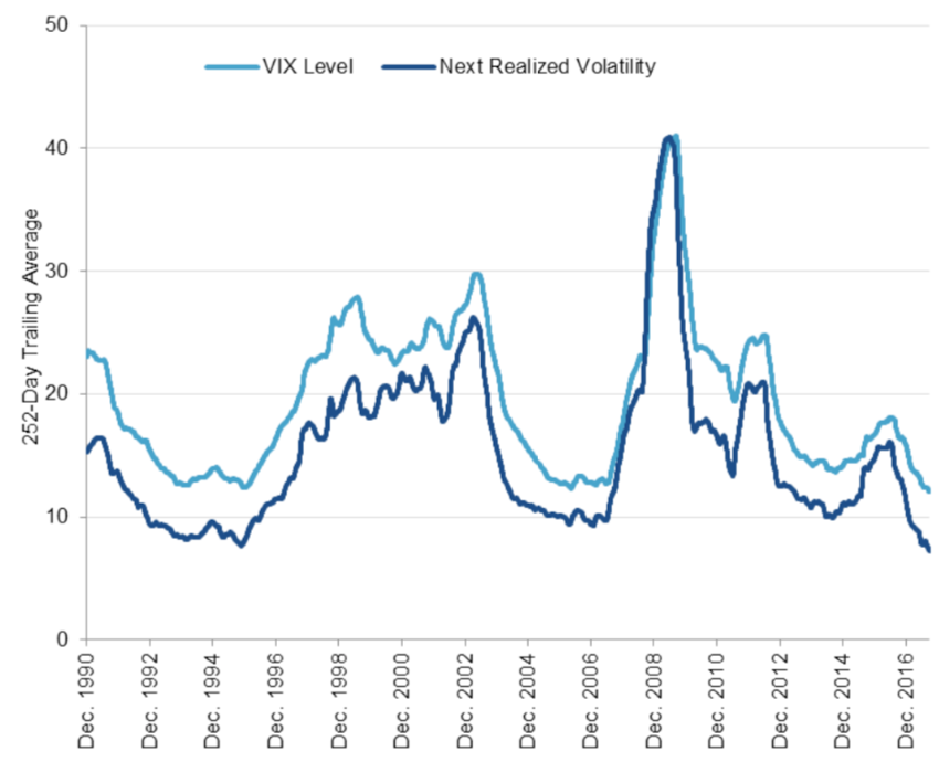
MSCI Value Factor Index

MSCI Factor Indexes are rules-based, transparent indexes that target equities with favorable factor qualities, as determined by academic discoveries and empirical outcomes, and are designed for easy implementation, replicability, and usage in both standard indexed and active portfolios. The stock price as a multiple of business earnings, the price as a multiple of dividends paid, the price as a multiple of book value, and other “ratio descriptors” are all examples of value. Academics and investors disagree on which business best symbolizes a value company, resulting in a market potential for a range of investment products. On a sector-by-sector basis, the MSCI Enhanced Value Index uses three valuation ratio descriptors:

Forward price to earnings (Fwd P/E)
Enterprise value/operating cash flows (EV/CFO)
Price to book value (P/B)

The index tries to avoid the problems of value investing, such as “value traps,” or stocks that look inexpensive but do not grow in value. The research demonstrates that whole-firm valuation metrics like enterprise value have decreased concentration in highly leveraged businesses (those that have taken on a lot of debt).

Performance of the MSCI Value Factor Index

Figure 1 compares the MSCI Value Factor Index’s performance to those of other factors from May 1999 to May 2020. All indices are rebalanced on a 100-point scale to ensure consistency in performance and to facilitate factor comparisons.

Figure 1. Performance of the MSCI Value Factor Index from 1999-2020.

Source: MSCI Factor research (2021).

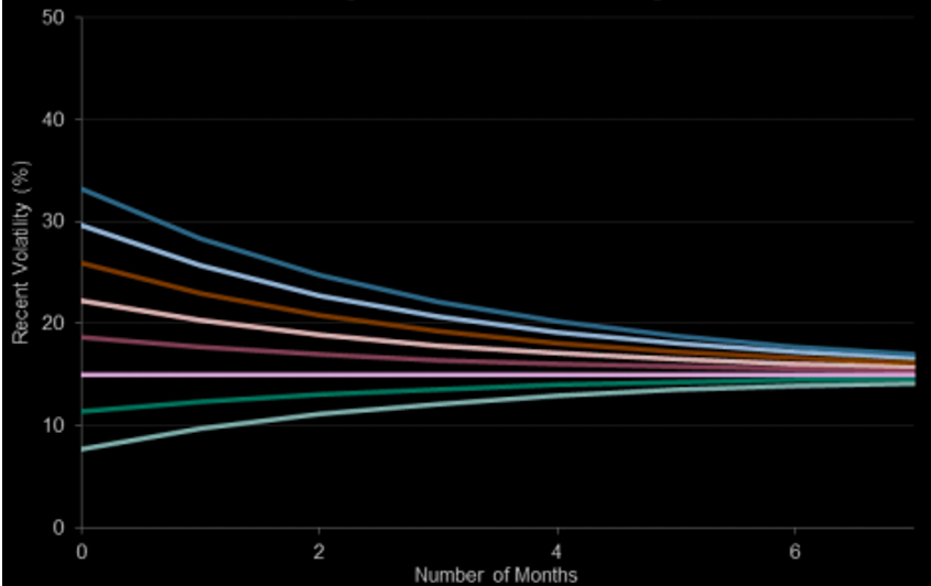
Since 1999, the MSCI World Enhanced Value Index has achieved excess returns above the MSCI World Index, with a 1.99 percent annual return over the MSCI World Index as seen above. (MSCI Factor research, 2021).

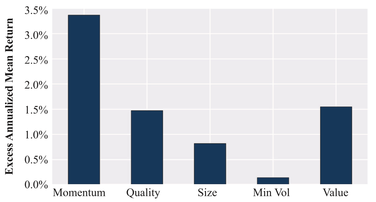
Risk-return profile of MSCI Value Factor Index

Figure 2 shows the MSCI Value Factor Index compared to other factors over the period May 1999 – May 2020 in terms of risk/reward. The risk-return tradeoff states that the potential return rises with an increase in risk. Individuals connect low levels of uncertainty about future returns with low potential returns, while high levels of uncertainty or risk are associated with large potential returns. According to the risk-tradeoff trade-off, an investor’s money can generate higher returns only if the investor is willing to endure a higher risk of loss (Figure 2).

Figure 2. Risk-return profile of MSCI Value Factor Index compared to a peer group.
Performance of the MSCI Value Factor Index from 1999-2020
Source: MSCI Factor research (2021).

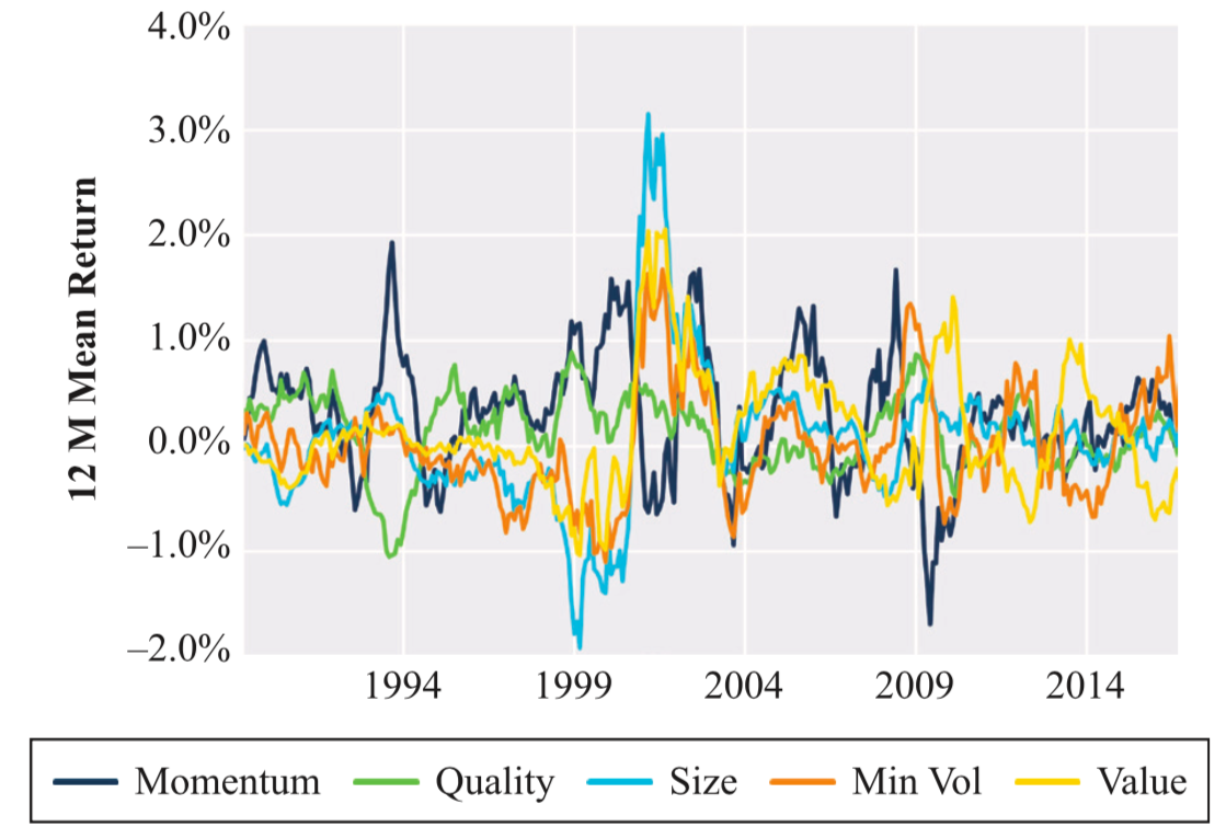
The basis of value investing is identifying stocks whose prices appear to understate their fundamental worth. While many institutional investors may agree, value-index strategies are executed in a number of ways. Incorporating the value factor into a portfolio might potentially boost returns and function as a well-researched performance vector (MSCI Factor research, 2021).

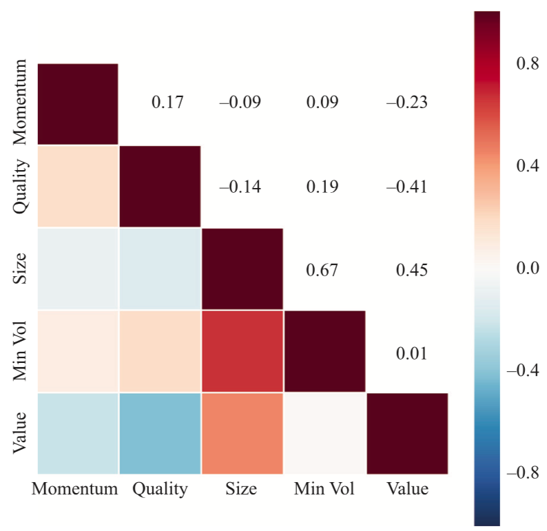
Behavior of the MSCI Value Factor Index during the Covid-19 crisis

Origin (01/11/2019 – 01/01/2020): the first instances are reported in Wuhan, China.
Incubation (02/01/2020 – 17/01/2020): during this phase, the number of patients began to rise at a faster rate, raising concerns about the disease’s severity.
Outbreak (20/01/2020 – 21/02/2020): the number of cases rose to the point that the World Health Organization (WHO) decided that this illness may pose a major threat to the world’s population, and the pandemic was proclaimed.
Fever (24/02/2020 – 20/03/2020): markets are extremely volatile, owing to government restrictions aimed at flattening the infection curve, with the decision to impose a lockdown in numerous nations as the most notable measures, among others.
Treatment (23/03/2020 – 15/04/2020): most of this turnaround occurs between March and June 2020, which corresponds with the start of good news about the discovery and widespread use of the vaccine.

Table 1. Performance of the MSCI factor indexes during the Covid-19 crisis.

Source: computation by the author. Data source: Thomson Reuters.

The value factor has performed not quite well in comparison to the other factors, finishing fourth out of five throughout the time period studied. Additionally, our study demonstrates that the value factor was the poorest performer during the incubation and outbreak stages and the second worst performer during the fever stage. This demonstrates the value factor’s instability during the Covid-19 crisis, which acted as a stress test.

ETFs to capture the Value factor

Figure 3 gives the overall ETF distribution of the major providers of value factor ETFs in terms of asset under management. By examining the market overview for minimal volatility factor investments, we can observe Blackrock (iShares) and State Street Global Advisors as the most dominant players in this segment. They hold nearly 50% and 34% respectively of the overall value factor ETF market, which underpins nearly 117B$ of the overall 138B$ in terms of market value for the value factor ETF market retained in this benchmark.

Figure 3. Value factor ETF market.

Source: etf.com (2021).

Table 2 gives more detailed information about the biggest value factor ETF providers: the asset under management (AUM), expense ratio (ER) and the segment for the investments.

Table 2. Ranking of the biggest Value ETF providers.

Source: etf.com (2021).

Why should I be interested in this post?

If you are an investor, you may consider adding an exposure to value factor to enhance the overall portfolio return.

Useful resources

Academic articles

Fama, E.F. French, K.R., 1992. The Cross-Section of Expected Stock Returns. The Journal of Finance , 47: 427-465.

Fama, E.F. French, K.R., 2015. A five-factor asset pricing model, Journal of Financial Economics , 116(1): 1-22.

Graham, B., Dodd, D., 1934. Security Analysis. 6th Edition, McGraw Hill.

Graham, B., 1949. The Intelligent Investor. 4th edition, Harper Business Essentials.

Hasaj, M., Sherer, B., 2021. Covid-19 and Smart-Beta: A Case Study on the Role of Sectors”. EDHEC-Risk Institute Working Paper.

Mangram, M.E., 2013. A simplified perspective of the Markowitz Portfolio Theory. Global Journal of Business Research, 7(1): 59-70.

Pagano, M., Wagner, C., Zechner, J. 2020. Disaster Resilience and Asset Prices, Working paper.

Business analysis

etf.com, 2021. Biggest Value Factor ETF providers.

MSCI Investment Research, 2021. Factor Focus: Value

Investopedia, 2021. Value Stock Definition.

About the author

The article was written in September 2021 by Youssef LOURAOUI (ESSEC Business School, Global Bachelor of Business Administration, 2017-2021).

My first experience in corporate finance inside a CAC40 group

About Bouygues

My experience at Bouygues

The process of rating

What I’ve learnt during this internship

Relevance to the SimTrade certificate

Related posts on the SimTrade blog

Useful resources

Academic articles

Business

About the author

Definition

Empirical study: monkeys vs passive mangers

Why should I be interested in this post?

Related posts on the SimSrade blog

Factor investing

Factor

Useful resources

Academic research

About the author

Introduction

Heuristic-based weighting strategies

Equal-weighting

Fundamental-weighting

Low beta weighting

Reverse-capitalization weighting

Maximum diversification

Optimization-based weighting strategies

Minimum Variance

Maximum Sharpe ratio

Why should I be interested in this post?

Related posts on the SimTrade blog

Factor investing

Factors

Useful resources

Academic research

About the author

Markowitz Modern Portfolio Theory

Modern Portfolio Theory

Assumptions of the Markowitz Portfolio Theory

Concepts used in the MPT

Risk

Systematic risk

Unsystematic risk

Risk-return trade-off

Diversification

Limitation of the model

Irrationality of investors

Relation between risk and expected return

Treatment of information by investors

Limitless Borrowing Capacity

Perfectly efficient markets

No Taxes or Transaction Costs

Conclusion

Why should I be interested in this post?

Related posts on the SimTrade blog

Portfolio Theory

Factor investing

Factors

Useful resources

Academic research

About the author

Smart Beta strategies: between active and passive allocation

Introduction

The passive investing approach

The active investing approach

Stock picking

Market timing

Review of academic literature

Passive investing

Active investing

Smart beta / factor investing

Case study: Comparison of market-capitalization-weighted portfolios and equally-weighted portfolios

Excel file for market-capitalization-weighted and equally-weighted portfolios

Smart beta: passive or active investment strategy?

Why should I be interested in this post?

Related posts on the SimTrade blog

Factor series

Useful resources

Academic research