Repo Rate

Repo Rate

Shruti CHAND

In this article, Shruti CHAND (ESSEC Business School, Grande Ecole Program – Master in Management, 2020-2022) elaborates on the concept of repo rate.

This read will help you get started with understanding repo rate and its significance.

What is Repo?

Repurchase rate is the rate at which the financial institutions in a country borrow and lend assets amongst themselves for a short-term. In the interbank market, the underlying security is sold by a bank to another in exchange of buying it the next day at a higher price on the following day usually. This exchange of the asset is facilitated by a contract known as “Repurchase agreement at a rate” or more commonly referred to “Repo”.

This agreement is similar to a loan agreement where the borrower of the loan pledges collateral with the lender for the time it borrows money and claims it back when the loan agreement is fulfilled. The underlying asset is usually a money market instrument such as Treasury bills and Treasury bonds. The main criteria to qualify as a collateral is that it should be liquid so that it can be sold in the open market if required.

Let us understand how a repurchase agreement works in detail:

The party of the contract who lends money in exchange of interests is known as the “repo seller”.

The borrower of the loan is known as the “repo buyer”.

The rate of the loan at which the lending is facilitated is known as the “repo rate”.

The collateral allows the lender to be protected against counter-party risk of the borrower. The value of the collateral is always higher than the amount lent to provide protection against market risk associated with collateral value. This additional amount is known as “haircut”.

Example

Let us illustrate this concept with an example:

Let us say Bank A (the borrower) is in dire need of liquid cash to facilitate an important transaction. In this scenario, it will turn to the Bank B (the lender) and request an amount of $100 m in cash.

Both banks decide to sign a repurchase agreement to facilitate this request. Bank B agrees to lend $100 m to Bank A and in return, Bank A agrees to pledge to Bank B Treasury bonds of a value higher than the value lent. This additional amount is known as ‘haircut’ as mentioned above. Let us assume in this case the haircut is $20 m, then the value of collateral that Bank A will keep for Bank B is equal to $120 m.

On day one, a repurchase agreement is signed between both banks. Bank A facilitates the agreement by holding the asset collateral with itself and Bank B lends cash to Bank A for its operations.

On day two, Bank A repays to Bank B the borrowed amount of $100 m and interests computed with the repo rate over one day. Let us assume the repo rate is equal to 5%. In this case, Bank A will pay $13,888 of interests to Bank B on day two and Bank B will free the collateral to Bank A.

Now that you understand a repo transaction, what is important also is to understand that a repo is one of the very important sources of funding for financial institutions in an economy. Central banks in every country use repurchase agreements to maintain liquidity level in the economy.

For example, the European Central Bank (ECB) sets three rates to keep the prices stable in the Euro zone. One of these rates is known as Refinancing option or Repurchasing option, which is an agreement to repurchase the collateral that the banks keep with the ECB of the country to borrow money for a very short period of time. Banks keep their Treasury bills or eligible securities with the Central Bank in exchange of money, they buy it later at a fixed price. ECB sets this rate every six weeks. This is how the policy makers for the Euro zone control the inflation level within the economy. On the other hand, opposite measures will be taken when the Central Bank needs to pump money in the economy.

Final Words

Repo rates are crucial to every economy and it differs based on various factors and is taken in control by policy makers whenever needed. As a student curious about Finance, learning about Repo Rate will go a long way in the future to understand better how liquidity and prices in the economy is maintained.

Relevance to the SimTrade certificate

This post deals with Repo Rate and how it is managed in the EU zone context.

About theory

  • By taking the SimTrade course , you will learn more about the markets. It’s important to remember that lending is a crucial part for investing.

Take SimTrade courses

About practice

  • By launching the series of Market maker simulations, you can extend your learning about financial markets and trading approaches.

Take SimTrade courses

About the author

Article written in August 2021 by Shruti CHAND (ESSEC Business School, Grande Ecole Program – Master in Management, 2020-2022).

Balance of Trade

Balance of Trades

Shruti CHAND

In this article, Shruti CHAND (ESSEC Business School, Grande Ecole Program – Master in Management, 2020-2022) elaborates on the concept of balance of trade.

This read will help you get started with understanding balance of trade and how it is practiced in today’s world.

Introduction

Balance of trade (BOT) refers to the difference between the monitory value of a country’s imports and exports over a specific period of time.

Imports refers to goods and services produced by another country and purchased by the domestic country for its consumption purposes whereas exports refer to the sale of goods and services produced by the domestic country to another country.

Balance of trade is the biggest part of the balance of payment (BOP). Balance of payment is the sum total of all the economic transactions of the residents of the country with the rest of the world. It includes capital movements, loan repayments, tourism, freight and insurance charges, and other payments. The payments and receipts of each country must be equal where any apparent quality simply leaves one country acquiring assets in the other.

Coming back to the balance of trade (also known as the ‘trade balance’, ‘international trade balance’, ‘commercial balance’ or the ‘net exports’) can result in a surplus (exports > imports) or in a deficit (imports > exports). When the exports of a country exceed its imports, the country is said to have a trade surplus. When the imports of a country exceed its exports, the country is said to have a trade deficit.

There have been constant changes in the economic theories revolving around
the balance of trade. According to the theory of mercantilism, a favorable/surplus balance of trade was necessary for ensuring the growth and well-being of an economy. It also symbolized a country’s wealth and power. However, this theory was soon challenged by classical economic theory of the late 18 th century when economists such as Adam Smith argued that free trade is more beneficial than the tendencies of mercantilism. The classical theory argued that countries are not quired to maintain a surplus in order to be more beneficial that is because a continuing surplus might in fact represent the underutilization of resources that could have otherwise contributed towards the country’s wealth.

Generally, developing countries have difficulty maintaining surpluses since the terms of trade during periods of recession are unfavorable for them. This is because they have to pay comparatively higher prices for finished goods that they import but receive lower prices for their exports of raw material or unfurnished goods.

Calculation of the Balance of Trade

The balance of trade is simply calculated as exports minus imports. It can be represented as follows:

TB = X – M where,

TB = Trade Balance
X = Exports (value of goods and services sold to the rest of the world)
M = Imports (value of goods and services purchased by the rest of the world)

When the exports are greater than imports it results in a trade surplus whereas when imports are greater than exports it results in a trade deficit. A country with a large trade deficit generally borrows money from other countries to balance the trade deficit while a country with large trade suppliers lends money to other nation for investing purposes. Generally, on a surface level, surplus is preferable to a deficit. But in reality, this might be an oversimplification. This is because a trade deficit might not inherently be bad,
as it can be an indicator of a strong economy. In addition to this, when we combine practical and sensible investment decisions, a deficit may lead to the stronger economic growth of a country in the future.

Interpretation for an Economy

In a basic sense, economists use balance of trade to measure the relative strength of a country’s economy. A country where imports are greater than exports face a trade deficit whereas a country where exports are greater than imports face a trade surplus.

But the reality of a situation is different when it comes to the interpretation of an economy based on the balance of trade. Sometimes a trade deficit can be unfavorable for a nation that focuses a lot on the export of raw material. As a result, this type of economy usually imports a lot of consumer products. As a consequence of the scene, the domestic businesses don’t attain the experiences needed to compete in the international market. Instead, the economy becomes increasingly dependent on global commodity prices, which can be highly volatile for such economy. Sometimes countries adopt the complete opposite of trade deficit when they follow the theory of mercantilism. In this scenario countries believe in maintaining a continuous surplus of trade in order to achieve the growth of the economy. It indulges in protective measures such as tariffs and import quotas to ensure the same. As a result, such measures can facilitate for a trade surplus, but a continuous trade surplus might result in higher cost for consumers, reduce international trade and may lead to diminishing economic growth.

Therefore, a positive or negative trade balance done does not necessarily indicate a healthy or a weak economy. Whether a trade surplus/deficit is beneficial for an economy or not depends on multiple factors such as the countries involved, trade policy decisions, the duration of the trade surplus/deficit, the size of the trade imbalance etc. For example, business cycles are an important factor to consider while interpreting the balance of trade. Because, in a recession, and economy tries to create more jobs and demand in the economy and as a result prefers to export more. On the contrary, during an economic expansion, countries prefer to import to promote price competition and as a direct consequence to limit inflation.

Related posts on the SimTrade blog

   ▶ Bijal GANDHI Economic indicators

   ▶ Bijal GANDHI Gross Domestic Product (GDP)

About the author

Article written by Shruti CHAND (ESSEC Business School, Grande Ecole Program – Master in Management, 2020-2022).

Online Brokers

Online Brokers

Shruti CHAND

In this article, Shruti CHAND (ESSEC Business School, Grande Ecole Program – Master in Management, 2020-2022) elaborates on the concept of online brokers.

This read will help you get started with understanding online brokers and how it is practiced in today’s world.

Introduction

A stockbroker is an entity that facilitates trading, that is to say executing trades on your behalf and storing your cash and stocks with them. Traditionally, brokers have been big banks and financial institutions that deal with billions of dollars in trading volumes. With advancing technology around the world, financial markets is adapting to the change, allowing retail investors to invest in the financial markets in new ways.

An online broker essentially is an entity that carries the activity of a broker without having a brick and motor existence, allowing its customers to execute and manage their trades by themselves on a trading platform available on the internet.

An online broker allows investors to trade in stocks, derivatives, commodities, cryptocurrencies, exchange-traded funds (ETFs), etc. in multiple currencies and markets. Additionally, they provide additional services such as:

  •  Market news
  •  Extensive investment information
  •  Expert advice
  •  Technical and fundamental analysis

online brokers provide their services in return of transactions and management fees, which are on the lower side for brokerage firms because of the low cost, they incur because of their non-physical existence. The expenses related to labor, property, management systems are reduced as all the process is carried out digitally. This allows the customers/investors to have quick transactions and a smooth experience. Some online brokers are in fact divisions of larger traditional brokers, e.g. Saxo Bank.

How can you use an online broker?

There are various online brokers available in every country which will allow you to use their platforms via their mobile phone application or internet website. Just as traditional brokers, they will make sure a robust system to study KYC (Know Your Customer) is conducted for every investor.

Additionally, regulators across the world are recognizing the potential of online brokers and making the system more secure day by day. The first step towards using an online brokerage is to choose the right one for you. In the US alone, with the growing number of online brokers, logins from mobile devices are up significantly between 35-50% over last year alone. There are various popular online brokers that one can start using, to begin with their investing journey.

Here, we have noted down attractive online brokers that investors use in
France:

1. Revolut- Has been transforming the online banking space and is one of the most convenient online brokers in terms of usage for beginners. It is FREE and easy to set up an account with them.

2. DEGIRO- Is in fact again one of the lowest fees trading platform. It is regulated by reputed authorities which makes it trustworthy and secured.

3. eToro- Very simple to open an account with them. It provides a simple to understand user interface and allows trading of almost all kinds of stocks, ETFs etc.

Steps to start availing services of an online broker:

1. Set up an account with an online broker
2. Get approved by the broker through a series of KYC and AML checks
3. Deposit the minimum amount of money to start trading.
4. Get additional support through reports, stock tracking, and investment advices.
5. Start investing.

It is sometimes argued that online brokers can be unsafe as their existence is not physical and the investors’ money can be lost if they go bust. The transition from traditional brokers to online brokers will take time but it is growing tremendously. Even the traditional brokers are opting for online facilities to match up with the trend.

Related posts on the SimTrade blog

   ▶ Wenxuan HU My experience as an intern of the Wealth Management Department in Hwabao Securities

   ▶ Akshit GUPTA Initial and maintenance margins in stocks

   ▶ Louis DETALLE A quick overview of the Bloomberg terminal…

Relevance to the SimTrade certificate

This post deals with online brokers which is used by various you as an investors in different instruments can use various mediums to invest in the markets:

About theory

  • By taking the Simtrade course, you will know more about how investors can use various strategies to invest in order to trade in the market.

Take SimTrade courses

About practice

  • By launching the series of Market maker simulations, you can extend your learning about financial markets and trading approaches.

Take SimTrade courses

About the author

Article written in August 2021 by Shruti CHAND (ESSEC Business School, Grande Ecole Program – Master in Management, 2020-2022).

High-frequency trading: pros and cons

High-frequency trading: pros and cons

Shruti CHAND

In this article, Shruti CHAND (ESSEC Business School, Grande Ecole Program – Master in Management, 2020-2022) elaborates on the concept of high-frequency trading.

This read will help you get started with understanding high-frequency trading and how it is practiced in today’s world.

What is it?

As the name suggests, the use of computer programs to place a large number of trades in fractions of a second (even thousandths of a second) is high-frequency trading or HFT.

These powerful programs have complex algorithms behind them, which analyze market conditions and place buy/sell orders in accordance with that.

The Upside

HFT improves market liquidity by reducing the bid-ask spread. This was put to test by adding fees on HFT, and in turn, bis-ask spreads increased. A study assessed how Canadian bid-ask spreads changed on the introduction of fees on HFT by the government, and it was found that market-wide bid-ask spreads increased by 13% and the retail spreads increased by 9%.

Stock exchanges, such as the New York Stock Exchange, offer incentives to market makers to perform HFT with the motive of increasing liquidity in the market. As a result of these financial incentives, the institutions that provide liquidity also see increased profits on each trade made by them, on top of their spreads.

Although the spreads and incentives amount to only a fraction of a cent per trade, multiplying that by a large number of trades per day amounts to sizable profits for high-frequency traders. In January 2021, the average Supplemental Liquidity Providers rebate was $0.0012 for securities traded on the NYSE. With millions of transactions each day, this results in a large number of profits.

The Flip Side

At one point in time, you can imagine HFT companies to be in heavy competition with each other to be the fastest, at the top of the game. Trading companies did everything from eliminating any possible inefficiency in the passage of signals from their IT equipment to the stock exchange; to relying on crunching more data to have an upper hand over their rivals. The boom years of this practice were in 2008 and 2009 when the difference between slower trading systems and the high-tech faster ones were in seconds. Now, all rivals have caught up and it is not as profitable of a business as it once was.

Besides this, HFT is also controversial and is faced with harsh criticism regarding ethical issues and their impact on market liquidity and market volatility as explained below.

Why is HFT criticized?

Critics believe HFT to be unethical. In their view, stock markets are supposed to offer a fair and level playing field, which HFT arguably disrupts as the technology can be used for ultra-short-term strategies. It has closed businesses for many broker-dealers; HFT is seen as an unfair advantage for large firms against smaller investors.

HFT is also said to provide ‘ghost liquidity’ i.e. the liquidity created by HFT in one second can be gone the next second, preventing traders from actually making use of the liquidity.

Moreover, a substantial body of research argues that HFT and electronic trading pose new kinds of challenges to the stability of financial markets. Algorithmic and high-frequency traders were both found to have had a contribution to volatility in the Flash Crash of May 2010, when high-frequency liquidity providers rapidly withdrew from the market. Several European countries have proposed restricting or fully banning HFT due to concerns about volatility.

Conclusion

It is very important to bear in mind the risk involved with high-frequency trading. With practice, you can become an expert, use SimTrade course to better your understanding about the financial markets to become a high-frequency trader.

Related posts on the SimTrade blog

   ▶ Akshit GUPTA High-frequency trading

   ▶ Akshit GUPTA Analysis of The Hummingbird Project movie

   ▶ Shruti CHAND Algorithmic trading

   ▶ Youssef LOURAOUI Quantitative equity investing

Relevance to the SimTrade certificate

This post deals with High-Frequency Trading which is used by various traders and investors in different instruments. This can be learned in the SimTrade Certificate:

About theory

  • By taking the market orders course , you will know more about how investors can use various strategies to invest in order to trade in the market.

Take SimTrade courses

About practice

  • By launching the series of Market maker simulations, you can extend your learning about financial markets and trading approaches.

Take SimTrade courses

About the author

Article written in August 2021 by Shruti CHAND (ESSEC Business School, Grande Ecole Program – Master in Management, 2020-2022).

Algorithmic Trading

Algorithmic Trading

Shruti Chand

In this article, Shruti Chand (ESSEC Business School, Master in Management, 2020-2022) elaborates on the concept of algorithmic trading.

This read will help you get started with understanding algorithmic trading and how it is practiced in today’s world.

What is it?

Today, as most activities of the world are moving towards (or already switched to) automation, trading is no different. The process of trading is automated using computer algorithms; which is basically a set of instructions. Trading algorithms are coded based on parameters such as stock price, volume, time, etc. When the current market conditions meet the criteria pre-defined in the algorithm, it executes a buy or sell order, without any human intervention. This is algorithmic trading.

Most algo-trading today is high-frequency trading (HFT), which attempts to capitalize on placing a large number of orders at rapid speeds (tens of thousands of trades per second) across multiple markets and multiple decision parameters based on preprogrammed instructions.

Some studies believe that around 92% of trading in the Forex market was performed by trading algorithms rather than humans.

New developments in artificial intelligence have enabled computer programmers to develop programs that can improve themselves through an iterative process called deep learning. Traders are developing algorithms that rely on this technique to make themselves more profitable.

How is it done?

We illustrate the implementation of algorithmic trading with two examples: technical analysis, arbitrage and market making.

Technical analysis:

Following trends in technical indicators such as moving average or price level movements is a safe and easy strategy used in programs in Algo-trading. There is no involvement of price predictions or forecasts.

Consider the following trade criteria:

  • Buy 100 shares of a stock when the 50-day moving average of the stock goes higher than its 200-day moving average (a moving average is basically the smoothening out of the price fluctuations by taking the average of previous data points, facilitating the identification of trends).
  • Sell the shares when the 50-day moving average of the stock goes lower than its 200-day moving average.

Using these two simple instructions, a computer program will automatically monitor the stock price (and the moving averages) and implement the buy and sell orders when the defined conditions are met. The trader no longer needs to painstakingly monitor live prices and graphs or put in the orders manually. This is done automatically by the algo-trading system by correctly identifying the trading opportunity.

Using 50-day and 200-day moving averages is a fairly popular trend-following strategy.

Arbitrage

To profit from arbitrage opportunities is a common strategy in algo-trading.

When a stock is listed in two different markets, you can buy shares at a lower price in one market and simultaneously sell them at a higher price in the other market. This offers the price differential as a risk-free profit, which defines an arbitrage. The same can be replicated for assets traded in the sport market and their futures in the derivatives market as the price differential may not exist from time to time. Implementing an algorithm to identify such price differentials and placing the orders efficiently helps seize profitable opportunities.

Market making

Besides that, algo-trading fairly affects how liquidity is provided to market participants as market making has been highly automized.

Other strategies

Besides these, there are various other strategies implemented by traders like Index Fund Rebalancing, Mathematical Model-based Strategies, Trading Range (Mean Reversion), Percentage of Volume (POV), etc.

Pros and Cons of Algorithmic Trading

Pros

Naturally, removing humans from the equation does have its undeniable merits.

The trading process becomes much faster and efficient. Additionally, the scope of human error is eliminated from the trading execution (although coding errors may still persist). Furthermore, the trades are not at risk of being driven by human emotions and other psychological factors.

Additionally, algo-trading significantly cuts down on costs associated with trading.

According to research, algorithmic trading is especially beneficial for large order sizes that may comprise as much as 10% of the overall trading volume.

Cons

While it has its advantages, algorithmic trading can also exacerbate the market’s negative tendencies by causing crashes (called “flash crash”) and immediate loss of liquidity.

The speed of order execution, an advantage in normal circumstances, can become a problem when several orders are executed simultaneously without human involvement. The flash crash of 2010 has been blamed on algo-trading.

Additionally, the liquidity that is created through rapid buy and sell orders, can disappear in a moment, eliminating the chance for traders to profit off-price changes. It can also cause instant loss of liquidity. Research has revealed that algorithmic trading was a major factor in causing a loss of liquidity in currency markets after the Swiss franc discontinued its euro peg in 2015.

Related posts on the SimTrade blog

   ▶ Youssef LOURAOUI Quantitative equity investing

   ▶ Rayan AKKAWI Big data in the financial sector

   ▶ Akshit GUPTA Market maker – Job Description

Relevance to the SimTrade certificate

This post deals with Algorithmic Trading which is used by various traders and investors in different instruments. This can be learned in the SimTrade Certificate:

About theory

  • By taking the market orders course , you will know more about how investors can use various strategies to invest in order to trade in the market.

Take SimTrade courses

About practice

  • By launching the series of Market maker simulations, you can extend your learning about financial markets and trading approaches.

Take SimTrade courses

About the author

Article written by Shruti Chand (ESSEC Business School, Master in Management, 2020-2022).

Value at Risk

Value at Risk

Jayati WALIA

In this article, Jayati WALIA (ESSEC Business School, Grande Ecole Program – Master in Management, 2019-2022) presents value at risk.

Introduction

Risk Management is a fundamental pillar of any financial institution to safeguard the investments and hedge against potential losses. The key factor that forms the backbone for any risk management strategy is the measure of those potential losses that an institution is exposed to for any investment. Various risk measures are used for this purpose and Value at Risk (VaR) is the most commonly used risk measure to quantify the level of risk and implement risk management.

VaR is typically defined as the maximum loss which should not be exceeded during a specific time period with a given probability level (or ‘confidence level’). Investments banks, commercial banks and other financial institutions extensively use VaR to determine the level of risk exposure of their investment and calculate the extent of potential losses. Thus, VaR attempts to measure the risk of unexpected changes in prices (or return rates) within a given period.

Mathematically, the VaR corresponds to the quantile of the distribution of returns on the investment.

VaR was not widely used prior to the mid 1990s, although its origin lies further back in time. In the aftermath of events involving the use of derivatives and leverage resulting in disastrous losses in the 1990s (like the failure of Barings bank), financial institutions looked for better comprehensive risk measures that could be implemented. In the last decade, VaR has become the standard measure of risk exposure in financial service firms and has even begun to find acceptance in non-financial service firms.

Computational methods

The three key elements of VaR are the specified level of loss, a fixed period of time over which risk is assessed, and a confidence interval which is essentially the probability of the occurrence of loss-causing event. The VaR can be computed for an individual asset, a portfolio of assets or for the entire financial institution. We detail below the methods used to compute the VaR.

Parametric methods

The most usual parametric method is the variance-covariance method based on the normal distribution.

In this method it is assumed that the price returns for any given asset in the position (and then the position itself) follow a normal distribution. Using the variance-covariance matrix of asset returns and the weights of the assets in the position, we can compute the standard deviation of the position returns denoted as σ. The VaR of the position can then simply computed as a function of the standard deviation and the desired probability level.

VaR Formula

Wherein, p represents the probability used to compute the VaR. For instance, if p is equal to 95%, then the VaR corresponds to the 5% quantile of the distribution of returns. We interpret the VaR as a measure of the loss we observe in 5 out of every 100 trading periods. N-1(x) is the inverse of the cumulative normal distribution function of the confidence level x.

Figure 1. VaR computed with the normal distribution.

VaR computed with the normal distribution

For a portfolio with several assets, the standard deviation is computed using the variance-covariance matrix. The expected return on a portfolio of assets is the market-weighted average of the expected returns on the individual assets in the portfolio. For instance, if a portfolio P contains assets A and B with weights wA and wB respectively, the variance of portfolio P’s returns would be:

Variance of portfolio

In the variance-covariance method, the volatility can be computed as the unconditional standard deviation of returns or can be calculated using more sophisticated models to consider the time-varying properties of volatility (like a simple moving average (SMA) or an exponentially weighted moving average (EWMA)).

The historical distribution

In this method, the historical data of past returns (for say 1,000 daily returns or 4 years of data) are used to build an historical distribution. VaR corresponds to the (1-p) quantile of the historical distribution of returns.
This methodology is based on the approach that the pattern of historical returns is indicative of future returns. VaR is estimated directly from data without estimating any other parameters hence, it is a non-parametric method.

Figure 2. VaR computed with the historical distribution.

VaR computed with the historical distribution

Monte Carlo Simulations

This method involves developing a model for generating future price returns and running multiple hypothetical trials through the model. The Monte Carlo simulation is the algorithm through which trials are generated randomly. The computation of VaR is similar to that in historical simulations. The difference only lies in the generation of future return which in case of the historical method is based on empirical data while it is based on simulated data in case of the Monte Carlo method.

The Monte Carlo simulation method is used for complex positions like derivatives where different risk factors (price, volatility, interest rate, dividends, etc.) must be considered.

Limitations of VaR

VaR doesn’t measure worst-case loss

VaR gives a percentage of loss that can be faced in a given confidence level, but it does not tell us about the amount of loss that can be incurred beyond the confidence level.

VaR is not additive

The combined VaR of two different portfolios may be higher than the sum of their individual VaRs.

VaR is only as good as its assumptions and input parameters

In VaR calculations especially parametric methods, unrealistic or inaccurate inputs can give misleading results for VaR. For instance, using the variance-covariance VaR method by assuming normal distribution of returns for assets and portfolios with non-normal skewness.

Different methods give different results

There are many approaches that have been defined over the years to estimate VaR. However, it essential to be careful in choosing the methodology keeping in mind the situation and characteristics of the portfolio or asset into consideration as different methods may be more accurate for specific scenarios.

Related posts on the SimTrade blog

   ▶ Jayati WALIA The variance-covariance method for VaR calculation

   ▶ Jayati WALIA The historical method for VaR calculation

   ▶ Jayati WALIA The Monte Carlo simulation method for VaR calculation

Useful Resources

Academic research articles

Artzner, P., F. Delbaen, J.-M. Eber, and D. Heath, (1999) Coherent Measures of Risk, Mathematical Finance, 9, 203-228.

Jorion P. (1997) “Value at Risk: The New Benchmark for Controlling Market Risk,” Chicago: The McGraw-Hill Company.

Longin F. (2000) From VaR to stress testing: the extreme value approach Journal of Banking and Finance, N°24, pp 1097-1130.

Longin F. (2016) Extreme events in finance: a handbook of extreme value theory and its applications Wiley Editions.

Longin F. (2001) Beyond the VaR Journal of Derivatives, 8, 36-48.

About the author

The article was written in September 2021 by Jayati WALIA (ESSEC Business School, Grande Ecole Program – Master in Management, 2019-2022).

Plain Vanilla Options

Plain Vanilla Options

Jayati WALIA

In this article, Jayati WALIA (ESSEC Business School, Grande Ecole Program – Master in Management, 2019-2022) presents plain vanilla options.

Introduction

An option contract is a financial derivative that gives its holder the right (but not the obligation) to trade an underlying asset at a price and a date set in advance.

In finance, plain vanilla refers to the most basic version of any financial instrument with standard features. Thus, a plain vanilla option simply refers to a contract that provides the option to buy or sell an underlying stock (or any financial asset) at a fixed price (known as the exercise/strike price) at an expiration date in the future. The expiration date (or maturity) of the option is the date when the holder can exercise her option if she wants.

In the US, options were first traded on an exchange on 26th April 1973. The Chicago Board Options Exchange (CBOE) was the first to create standardized, listed options. Today, there are over 50 exchanges worldwide that trade options.

When an option is bought, its holder pays a fixed amount to the option writer as the cost for the flexibility of trading that the option provides. This cost, which is essentially the value of an option (and the margin taken by the issuer), is known as the premium. The premium depends on the characteristics of the option like the strike price and the maturity, and on market data like the price of the underlying asset and especially its volatility. Many different underlying assets can be traded through options including stocks, bonds, commodities, foreign currencies.

Types of options

Vanilla options are of two types: call and put.

Call options

The holder of a call option has the right to buy a particular asset at a strike price K at maturity T. If the asset price at maturity denoted by ST is higher than K, then it is beneficial for the call option holder to exercise his option at time T as the price set in the call option contract K is lower than the market price ST. If the asset price at maturity ST is lower than K, then it is not beneficial for the call option holder to exercise his option at time T as the price set in the call option contract K is higher than the market price ST; he is then better off to buy the asset on the market at price ST than at price K.

For example, consider a call option on BNP Paribas stock with a strike price of €50 and a maturity date March 31st. The holder of this call option thus has the right but not the obligation to buy one BNP Paribas stock for €50 at maturity. He will exercise his option on March 31st if and only if the stock price is higher than €50.

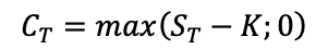
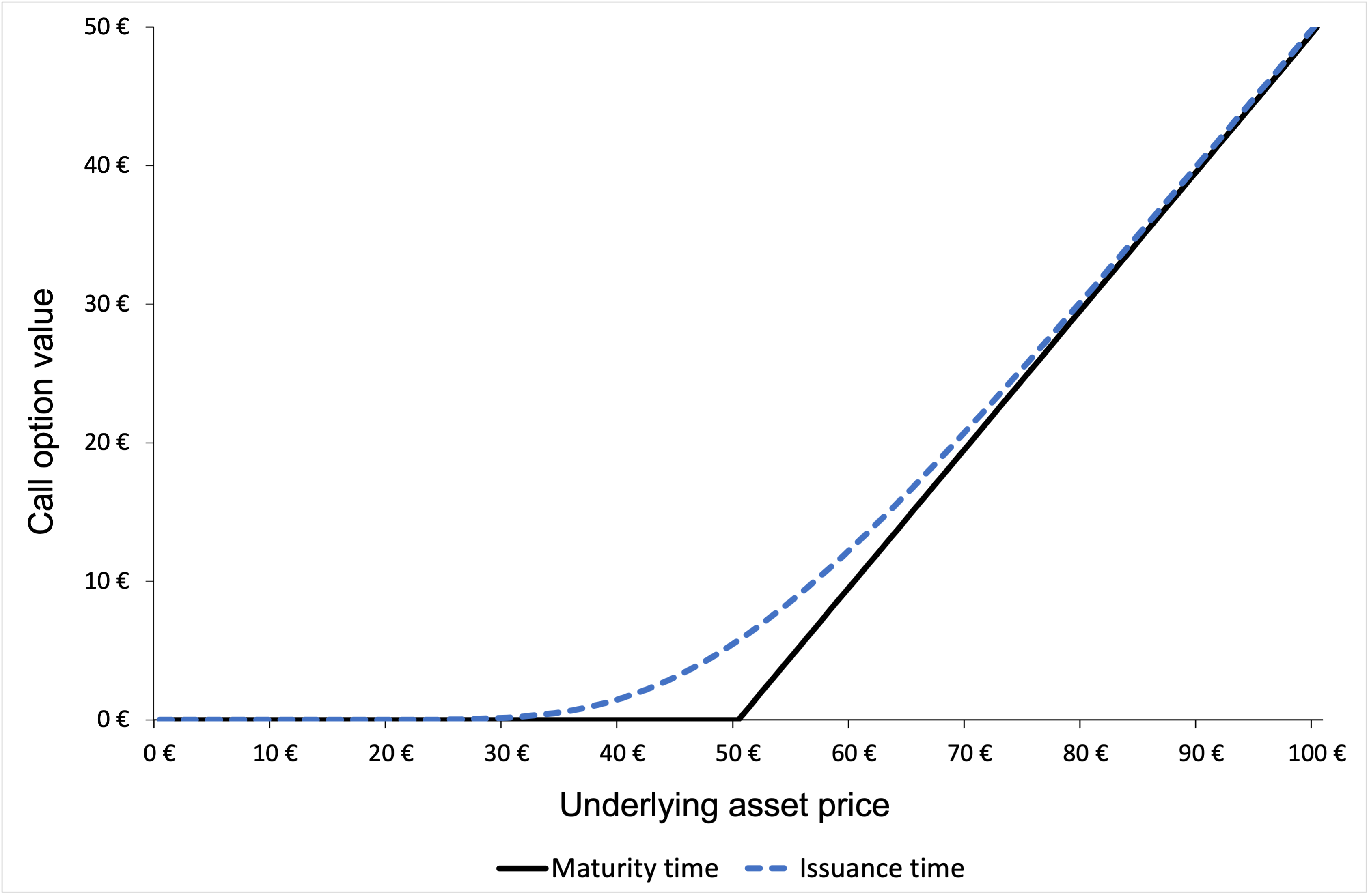
The equation below gives the pay-off function of a call option that is the value of the call option at maturity T denoted by CT as a function of the price of the underlying asset ST.

Payoff formula for a call option

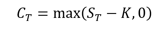
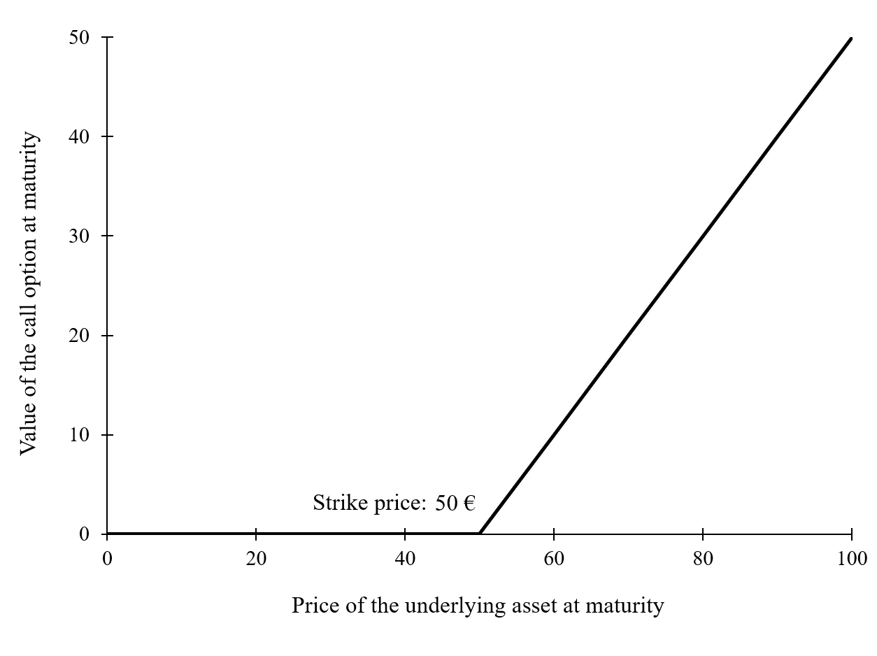
Figure 1 gives a graphical representation of the pay-off function of a call option that is the value of the call option at maturity T as a function of the price of the underlying asset at maturity T, ST, for a given strike price (equal to €50 in the figure).

Figure 1. Pay-off function of a call option

 Payoff for a call option

Put options

Similarly, the holder of a put option has the right to sell a particular asset at a strike price K at maturity T. If the asset price at maturity denoted by ST is higher than K, then it is beneficial for the put option holder not to exercise his option at time T as the price set in the put option contract K is lower than the market price ST; he is then better off to sell the asset on the market at price ST than at price K. If the asset price at maturity ST is lower than K, then it is beneficial for the put option holder to exercise his option at time T as the price set in the put option contract K is higher than the market price ST.

For example, consider a put option on BNP Paribas stock with a strike price of €50 and a maturity date March 31st. The holder of this put option thus has the right but not the obligation to sell one BNP Paribas stock for €50 at maturity. He will exercise his put option on March 31st if and only if the stock price is lower than €50.

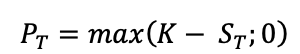
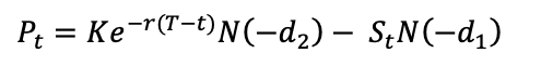
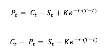
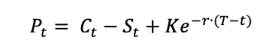
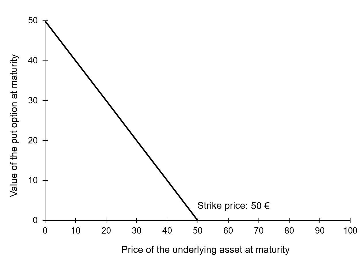
The equation below gives the pay-off function of a put option that is the value of the put option at maturity T denoted by PT as a function of the price of the underlying asset ST.

Payoff formula for a put option

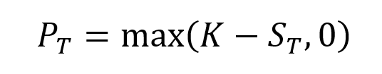
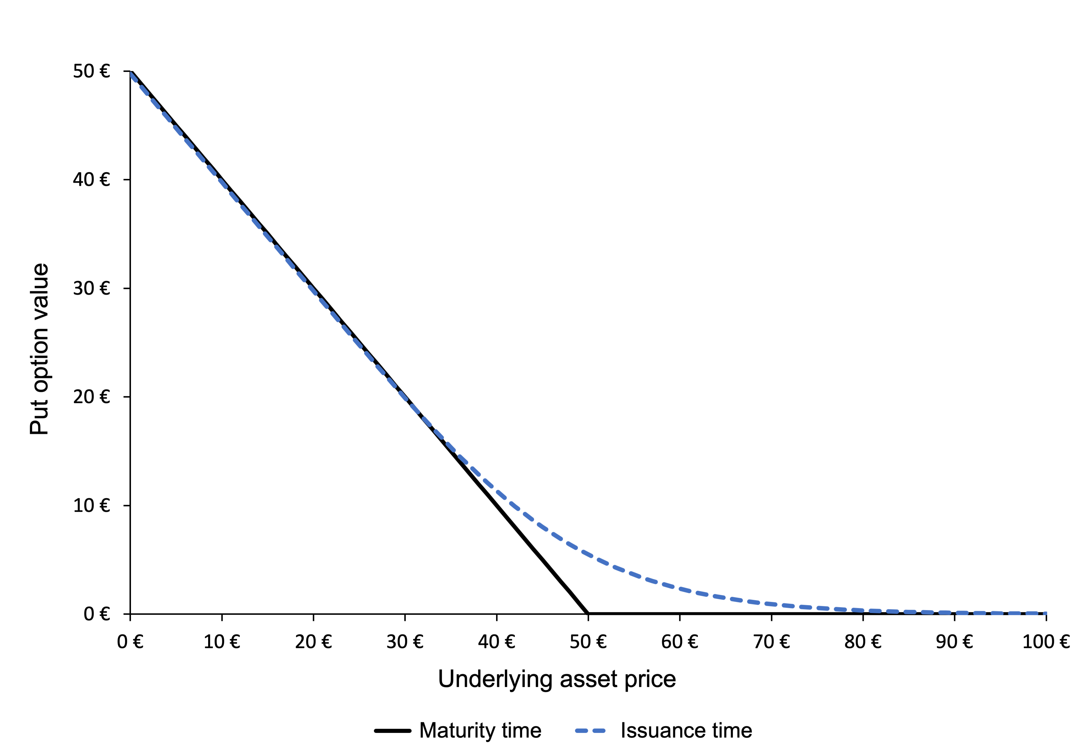
Figure 2 gives a graphical representation of the pay-off function of a put option that is the value of the put option at maturity T as a function of the price of the underlying asset ST for a given strike price (equal to €50 in the figure).

Figure 2. Pay-off function of a put option

 Payoff for a put option

Types of exercise

Options can be categorized based on their exercise restrictions.

American options

American options have the most flexible arrangement allowing holders to exercise their options at any time prior to the expiration date. They are widely traded over listed exchanges.

European options

European options provide less flexibility and allow holders to exercise options on only one specific date, which is the expiration date. They thus have a lower value compared to American options and are generally traded OTC.

Bermudan options

There are also Bermudan options that allow exercise of options on a set of specific dates before the expiration and thus provide holders a level of flexibility midway between American and European Options.

Moneyness

Options can also be characterized by their “moneyness” which compares the current price of the underlying asset to the option strike.

In-the-money options

An option with a positive intrinsic value is said to be ‘in the money’. This is the case for a call option if the current market price of the asset is higher than the strike price, and similarly for a put option if the current market price of the asset is lower than the strike price.

Out-of-the-money options

An option with a zero intrinsic value is said to be ‘out of the money’. This is the case for a call option if the current market price of the asset is lower than the strike price, and similarly for a put option if the current market price of the asset is higher than the strike price.

At-the-money options

An option with a strike price close or equal to the current market price is said to be ‘at the money’.

Option writers

The above discussion mainly revolves around option purchasers. However, there is also someone who is liable to sell (for a call) or buy (for a put) the underlying security whenever any holder exercises an option. The writer of an option is the person who is obligated to buy/sell the underlying in case of a call/put exercise. As a counterpart, the writer also receives the option premium from the holder.

The best-case scenario for a writer would be that the option is not exercised by its holder as the option remains out of the money (the writer earning the premium without being obliged to pay the cash flow at maturity). However, option writers are exposed to downside risks especially if the options they write are not covered i.e., holding a long or short position already in the underlying security depending on the option written.

Benefits

For traders with strong market views looking to leverage benefits from small to medium-term fluctuations in market price, buying options is an efficient means to offset their risk exposure. The buyer only risks a small amount of investment, and the downside is only limited to the initial premium whereas the upside is a high payoff if the speculation is in her/his favor. The traders can also take up multiple positions in different assets through options and leverage trade opportunities with profitable positions covering more than the hedging costs.

Option Trading

Most vanilla options are traded through exchanges that make it convenient to match buyers with sellers and vice versa. Trading of standardized contracts also promotes liquidity of the instruments in the market. Vanilla options generally come in series of standardized strike prices and expiration dates. For instance, for an option contract on an Apple Inc. stock (AAPL) expiring on 20th August 2021, the offered strike prices are $115, $120, $125, $130 and so on. Similarly, the expiration dates for listed stock options is generally the third Friday of the month in which the contract expires. If the Friday falls on a holiday, the expiration date becomes Thursday immediately before the third Friday.
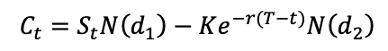
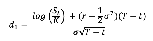
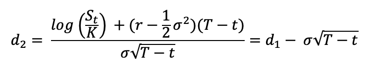
Option pricing

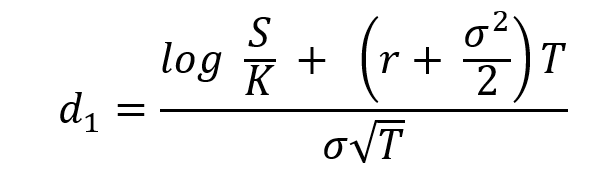
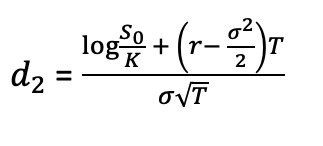
The value an option is known at maturity as it is given by the contract. But what is the value of an option at the time of its issuance or at a time before maturity? Many mathematical models have been developed to answer this question. The most famous model is the Black-Scholes-Merton option pricing model. It uses a Brownian motion to model the behavior of stock market prices.

Use of options

Hedging

Options are commonly used in hedging. For instance, you can purchase an option on a stock to limit your losses to say 15% of your position, should the stock decline more than that during the option period.

Speculation

If one has a strong view about the potential market direction of an underlying security, one can make great returns on exploiting options, provided the view was right. This is essentially speculation in option trading. For instance, if you have a bullish opinion regarding a stock, you can purchase a call option on it that will allow you to purchase the stock at the strike price that will be lower than the future price (hopefully!). Thus, if you are right, you could exercise the option and your payoff would be the price difference between the stock price and the strike price. If you are wrong, you lose out on the premium you paid for the option.
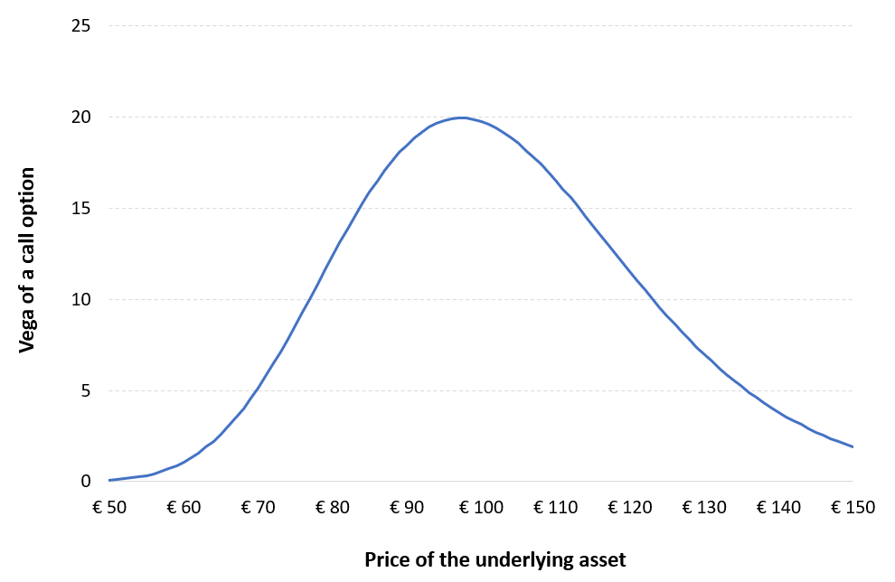
Volatility

The volatility of the underlying asset affects positively option prices: stocks with higher volatility have more expensive option contracts that those with low volatility. In fact, the implied volatility (IV) of an option is that value of the volatility of the underlying instrument for which an option pricing model (such as the Black-Scholes-Merton model) will return a theoretical value equal to the current market price of that option. Hence, when the implied volatility increases, the price of options increases as well, assuming all other factors remain constant. When the implied volatility increases after a trade has been placed, it is good news for the option owner and, conversely bad news for the seller. Inversely, when the implied volatility decreases after a trade has been placed, it is bad news for the option owner and, conversely good news for the seller.

Note that the implied volatility tends to depend on the strike price and maturity date of the options for a given underlying asset. Once the implied volatility for the at-the-money contracts is determined in any given expiration month, market makers use pricing models and volatility skews to calculate implied volatility at other strike prices that are less heavily traded. So, every option has an associated volatility and risk profiles can vary drastically among options. Traders may at times balance out the risk of volatility by hedging one option with another.

Thus, it is essential to interpret and analyze risks before venturing into option trading. There are also many strategies that can be applied to vanilla options in order to benefit better and limit risk such as long and short calls/puts, bull and bear spreads, straddles and strangles, butterflies, condors among many.

Related posts on the SimTrade blog

All posts about Options

▶ Jayati WALIA Derivatives Market

▶ Jayati WALIA Black-Scholes-Merton option pricing model

▶ Jayati WALIA Brownian Motion in Finance

Useful Resources

Nasdaq Historical data for Apple stock

AVATRADE What are vanilla options

TheStreet Options Trading

About the author

The article was written in August 2021 by Jayati WALIA (ESSEC Business School, Grande Ecole Program – Master in Management, 2019-2022).

Derivatives Market

Derivatives Market

Jayati WALIA

In this article, Jayati WALIA (ESSEC Business School, Grande Ecole Program – Master in Management, 2019-2022) presents an overview of derivatives market.

Introduction

A financial market refers to a marketplace where various kinds of financial securities such as stocks, bonds, commodities, etc. are traded. The term ‘market’ can also refer to exchanges that are legal organizations that facilitate the trade of financial securities between buyers and sellers. In any case, these markets are categorized based of the type of financial securities that are traded through them. One such financial market is the Derivatives Market.

Derivatives market thus refers to the financial marketplace where derivative instruments such as futures, forwards and options contracts are traded between counterparties.

It was during the 1980s and 1990s that the financial markets saw a major growth in the trade of derivatives. A derivative is a financial instrument whose value is derived from the value of an underlying asset such as stocks, bonds, currencies, commodities, interest rates and/or different market indices. These underlying assets have fluctuating prices and returns, and derivatives provides a means to investors to reduce the risk exposure and leverage profits on these assets. Thus, derivatives are an essential class of financial instruments and central to the modern financial markets providing not just economic benefits but also resilience against risks. The most common derivatives include futures, forwards, options and swap contracts.

As per the European Securities and Markets Authority (ESMA), derivatives market has grown impressively (around 24 percent per year in the last decade) into a truly global market with over €680 trillion of notional amount outstanding. The interest rate derivatives (IRDs) accounted for 82% of the total notional amount outstanding followed by currency derivatives at 11%.

Main types of derivative contracts

Derivatives derive their value from an underlying asset, or simply an ‘underlying’. There is a wide range of financial instruments that can be an underlying for a derivative such as equities or equity index, fixed-income instruments, foreign currencies, commodities, and even other securities. And thus, depending on the underlying, derivative contracts can derive their values from corresponding equity prices, interest rates, foreign exchange rates, prices of commodities and probable credit events. The most common types of derivative contracts are elucidated below:

Forwards and Futures

Forward and futures contracts share a similar feature: they are an agreement between two parties to buy or sell a specified quantity of an underlying asset at a specified price (or ‘exercise price’) on a predetermined date in the future (or ‘expiration date’). While forwards are customized contracts i.e., they can be tailor-made according to the asset being traded, expiry date and price, and traded Over-the-Counter (OTC), futures are standardized contracts traded on centralized exchanges. The party that buys the underlying is said to be taking a long position while the party that sells the asset takes a short position and both parties are obligated to fulfil their part of the contract.

Options

An option contract is a financial derivative that gives its holder the right (but not the obligation) to trade an underlying asset at a price set in advance irrespective of the market price at maturity. When an option is bought, its holder pays a fixed amount to the option writer as cost for this flexibility of trading that the option provides, known as the premium. Options can be of the types: call (right to buy) or put (right to sell).

Swaps

Swaps are agreements between two counterparties to exchange a series of cash payments for a stated period of time. The periodic payments charged can be based on fixed or floating interest rates, depending on contract terms decided by the counterparties. The calculation of these payments is based on an agreed-upon amount, called the notional principal amount (or just notional).

Exchange-traded vs Over-the-counter Derivatives Market

Exchange-traded derivatives markets

Exchange-traded derivatives markets are standardized markets for derivatives trading and follows rules set by the exchange. For instance, the exchange sets the expiry date of the derivatives, the lot-size, underlying securities on which derivatives can be created, settlement process etc. The exchange also performs the clearing and settlement of trades and provide credit guarantee by acting as a counterparty for every trade of derivatives. Thus, exchanges provide a transparent and systematic course of action for any derivatives trade.

Over-the-counter markets

Over-the-counter (also known as “OTC”) derivatives markets on the other hand, provide a lesser degree of regulations. They were almost entirely unregulated before the financial crisis of 2007-2008 (also a time when derivatives markets were criticized, and the blame was placed on Credit Default Swaps). OTCs are customized markets and run by dealers who hedge risks by indulging in derivatives trading.

Types of market participants

The participants in the derivative markets can be categorized into different groups namely,

Hedgers

Hedging is a risk-neutralizing strategy when an investor seeks to protect a current or anticipated position in the market by limiting their risk exposure. They can do so by taking up an offset or counter position through derivative contracts. Parties such as individuals or companies who perform hedging are called Hedgers. The hedger thus aims to eliminate volatility against fluctuating prices of underlying securities and protect herself/himself from any downsides.

Speculators

Speculation is a very common technique used by traders and investors in the derivatives market. It is based on when traders have a strong viewpoint regarding the market behavior of any underlying security and though it is risky, if the viewpoint is correct, the speculation may reward with attractive payoffs. Thus, speculators use derivative contracts with a view to make profit from the subsequent price movements. They do not have any risk to hedge, in fact, they operate at a relatively high-risk level in anticipation of profits and provide liquidity in the market.

Arbitrageurs

Arbitrage is a strategy in which the participant (or arbitrageur) aims to make profits from the price differences which arise in the investments made in the financial markets as a result of mispricing. Arbitrageurs aim to earn low risk profits by taking two different positions in the same or different contracts (across different time periods) or on different exchanges to in-cash on price discrepancies or market inefficiencies.

Margin Traders

Margin is essentially the collateral amount deposited by an investor investing in a financial instrument to the counterparty in order to cover for the credit risk associated with the investment. In margin trading, the trader or investor is not required to pay the total value of your position upfront. Instead, they only need pay the margin amount which may vary and are usually fixed by the stock exchanges considering factors like volatility. Thus, margin traders buy and sell securities over a single session and square off their position on the same day, making a quick payoff if their speculations are right.

Criticism of derivatives

While derivatives provide numerous benefits and have significantly impacted modern finance and markets, they pose many risks too. In a 2002 letter to Berkshire Hathaway shareholders, Warren Buffet even described derivatives as “financial weapons of mass destruction”.

Derivatives are more highly leveraged due to relatively relaxed regulations surrounding them, and where one may need to put up half the money or more with buying other securities, derivatives traders can get by with just putting up a few percentage points of the total value of a derivatives contract as a margin. If the price of the underlying asset keeps falling, covering the margin account can lead to enormous losses. Derivatives are thus often criticized as they may allow investors to obtain unsustainable positions that elevates systematic risk so much that it can be equated to legalized gambling. Derivatives are also exposed to counterparty credit risk wherein there is scope of default on the contract by any of the parties involved in the contract. The risk becomes even greater while trading on OTC markets which are less regulated.

Derivatives have been associated with a number of high-profile credit events over the past two decades. For instance, in the early 1990s, Procter and Gamble Corporation lost more than $100 million in transactions in equity swaps. In 1995, Barings collapsed when one of its traders lost $1.4 billion (more than twice its then capital) in trading equity index derivatives.

The amounts involved with derivatives-related corporate financial distresses in the 2000s increased even more. Two such events were the bankruptcy of Enron Corporation in 2001 and the near collapse of AIG in 2008. The point of commonality among these events was the role of OTC derivative trades. Being an AAA-rated company, AIG was being exempted from posting collateral on most of its derivatives trading in 2008. In addition, AIG was unique among CDS market participants and acted almost exclusively as credit protection seller. When the global financial crisis reached its peak in late 2008, AIG’s CDS portfolios recorded substantial mark-to-market losses. Consequently, the company was asked to post $40 billion worth of collateral and the US government had to introduce a $150 billion financial package to prevent AIG, once the world’s largest insurer by market value, from filing for bankruptcy.

Conclusion

Derivatives were essentially created in response to some fundamental changes in the global financial system. If correctly handled, they help improve the resilience of the system, hedge market risks and bring economic benefits to the users. Thus, they are expected to grow further with financial globalization. However, past credit events have exposed many weaknesses in the organization of their trading. The aim is to minimize the risks associated with such trades while enjoying the benefits they bring to the financial system. An important challenge is to design new rules and regulations to mitigate the risks and to promote transparency by improving the quality and quantity of statistics on derivatives markets.

Related posts on the SimTrade blog

   ▶ All posts about Options

   ▶ Alexandre VERLET Understanding financial derivatives: options

   ▶ Jayati WALIA Plain Vanilla Options

   ▶ Alexandre VERLET Understanding financial derivatives: forwards

   ▶ Alexandre VERLET Understanding financial derivatives: futures

   ▶ Alexandre VERLET Understanding financial derivatives: swaps

Useful resources

Role of Derivatives in the 2008 Financial Crisis

ESMA Annual Statistical Report 2020

About the author

The article was written in August 2021 by Jayati WALIA (ESSEC Business School, Grande Ecole Program – Master in Management, 2019-2022).

Linear Regression

Linear Regression

Jayati WALIA

In this article, Jayati WALIA (ESSEC Business School, Grande Ecole – Master in Management, 2019-2022) presents linear regression.

Definition

Linear regression is a basic and one of the commonly used type of predictive analysis. It attempts to devise the relationship between two variables by fitting a linear function to observed data. A simple linear regression line has an equation of the form:


wherein Y is considered to be the dependent variable (i.e., variable we want to predict) and X is the explanatory variable (i.e., the variable we use to predict the dependent variable’s value). The slope of the line is β1, and β0 is the x-intercept. ε is the residual (or error) in prediction.

Application in finance

For instance, consider Apple stock (AAPL). We can estimate the beta of the stock by creating a linear regression model with the dependent variable being AAPL returns and explanatory variable being the returns of an index (say S&P 500) over the same time period. The slope of the linear regression function is our beta.

Figure 1 represents the return on the S&P 500 index (X axis) and the return on the Apple stock (Y axis), and the regression line given by the estimation of the linear regression above. The slope of the linear regression gives an estimate of the beta of the Apple stock.

Figure 1. Example of beta estimation for an Apple stock.

Beta_AAPL

Source: computation by the author (Data: Apple).

Before attempting to fit a linear model to observed data, it is essential to determine some correlation between the variables of interest. If there appears to be no relation between the proposed independent/explanatory and dependent, then the linear regression model will probably not be of much use in the situation. A numerical measure of this relationship between two variables is known as correlation coefficient, which lies between -1 and 1 (1 indicating positively correlated, -1 indicating negatively correlated, and 0 indicating no correlation). A popularly used method to evaluate correlation among the variables is a scatter plot.

The overall idea of regression is to examine the variables that are significant predictors of the outcome variable, the way they impact the outcome variable and the accuracy of the prediction. Regression estimates are used to explain the relationship between one dependent variable and one or more independent variables and are widely applied to domains in business, finance, strategic analysis and academic study.

Assumptions in the linear regression model

The first step in the process of establishing a linear regression model for a particular data set is to make sure that the in consideration can actually be analyzed using linear regression. To do so, our data set must satisfy some assumptions that are essential for linear regression to give a valid and accurate result. These assumptions are explained below:

Continuity

The variables should be measured at a continuous level. For example, time, scores, prices, sales, etc.

Linearity

The variables in consideration must share a linear relationship. This can be observed using a scatterplot that can help identify a trend in the relationship of variables and evaluate whether it is linear or not.

No outliers in data set

An outlier is a data point whose outcome (or dependent) value is significantly different from the one observed from regression. It can be identified from the scatterplot of the date, wherein it lies far away from the regression line. Presence of outliers is not a good sign for a linear regression model.

Homoscedasticity

The data should satisfy the statistical concept of homoscedasticity according to which, the variances along the best-fit linear-regression line remain equal (or similar) for any value of explanatory variables. Scatterplots can help illustrate and verify this assumption

Normally-distributed residuals

The residuals (or errors) of the regression line are normally distributed with a mean of 0 and variance σ. This assumption can be illustrated through a histogram with a superimposed normal curve.

Ordinary Least Squares (OLS)

Once we have verified the assumptions for the data set and established the relevant variables, the next step is to estimate β0 and β1 which is done using the ordinary least squares method. Using OLS, we seek to minimize the sum of the squared residuals. That is, from the given data we calculate the distance from each data point to the regression line, square it, and calculate sum of all of the squared residuals(errors) together.

Thus, the optimization problem for finding β0 and β1 is given by:

After computation, the optimal values for β0 and β1 are given by:

Using the OLS strategy, we can obtain the regression line from our model which is closest to the data points with minimum residuals. The Gauss-Markov theorem states that, in the class of conditionally unbiased linear estimators, the OLS estimators are considered as the Best Linear Unbiased Estimators (BLUE) of the real values of β0 and β1.

R-squared values

R-squared value of a simple linear regression model is the rate of the response variable variation. It is a statistical measure of how well the data set is fitted in the model and is also known as coefficient of determination. R-squared value lies between 0 and 100% and is evaluated as:

The greater is the value for R-squared, the better the model fits the data set and the more accurate is the predicted outcome.

Useful Resources

Linear regression Analysis

Simple Linear Regression

Related Posts

   ▶ Louraoui Y. Beta

About the author

The article was written in August 2021 by Jayati WALIA (ESSEC Business School, Grande Ecole – Master in Management, 2019-2022).

The Black Scholes Merton Model

The Black-Scholes-Merton model

Akshit Gupta

This article written by Akshit GUPTA (ESSEC Business School, Grande Ecole Program – Master in Management, 2019-2022) presents the Black-Scholes-Merton Model .

Introduction

Options are one of the most popular derivative contracts used by investors to hedge the risks of their portfolios, to optimize the risk profile of their positions and to make profits (or losses) by means of speculation. The value of options is known at maturity date (or expiration date) as it is given by their pay-off functions defined in their contracts. But what is the value of the option at the issuance date or any date between the issuance and the expiration? The Black-Scholes-Merton model allows to answer this question.

The Black-Scholes-Merton model is an continuous-time option pricing model used to determine the fair price or theoretical value for a call or a put option based on variable factors such as the maturity date and the strike price of the option (option characteristics), and the price of underlying asset, the volatility of the price of underlying asset, and the risk-free rate (market data). It is used to determine the price of a European call option, which refers to the option that can only be exercised on the maturity date.

History

The model was first introduced to the world by a paper titled ‘The Pricing of Options and Corporate Liabilities’ by Fischer Black and Myron Scholes and was officially published in spring 1973. Almost around the same time as Black and Scholes, Robert Merton, who was also a colleague of Scholes at MIT Sloan, presented his contributions to the model in another paper named ‘Theory of Rational Option Pricing’, where he coined the name “Black-Scholes model”. Later, Black and Scholes also published empirical tests of the model in their ‘The Valuation of Option Contracts and a Test of Market Efficiency’ paper. For their significant contribution to the world of financial markets, Merton and Black were awarded the prestigious Nobel Prize in Economic Sciences in 1997 (unfortunately Scholes had passed away in 1995 due to which he was ineligible for the Nobel Prize).

In the BSM model, the value of an option depends on the future volatility of the underlying stock rather than on its expected return. The pricing formula is based on the assumption that the price of the underlying asset follows a geometric Brownian motion.

Option pricing with BSM

The BSM model is used to find the theoretical value of a European option. The model assumes that the price of the underlying asset follows a geometric Brownian motion, which implies that the returns on the underlying asset are normally distributed. It is also assumed that there are no arbitrage opportunities, no transaction costs and the risk-free rate remains constant over time.

The BSM formula

The payoffs for a call option and a put option give the value of these options at the maturity date T:

For a call option:

Formula for the payoff of a call option

For a put option:

BSM Formula for the payoff of a put option

The BSM formula gives the price of European put and call options at any date before the maturity date T. The value of European call and put options for a non-dividend paying stock are given by:

For a call option:

BSM formula for the call option

For a put option:

BSM formula for the put option

where,

Formula for the D1Formula for the D2

The notations used in the above formulae are described as :

St: price of the underlying asset at time t
t: current date (or date of calculation of option price)
T: maturity or expiry date of the option
K: strike price of the option
r: risk-free interest rate
σ: volatility (the standard deviation of the return on the underlying asset)
N(.): cumulative distribution function for a normal (Gaussian) distribution (0 ≤ N(.) ≤ 1 )

For a call option, N(+d2) is the probability that the option will be exercised, and Ke(-r(T-t) ) N(+d2) is what is expected to be paid for the underlying stock if the option is exercised, discounted to today (or the calculation date t).

Similarly, SN(+d1) is what we can expect to receive from selling the underlying stock, if the option is exercised, also discounted to today (or the calculation date t).

For a put option, N(-d2) is the probability that the option will be exercised, and Ke(-r(T-t) ) N(-d1 ) is what is expected to be paid for the underlying stock if the option is exercised, discounted to today (or the calculation date t).

Similarly, SN(-d1 ) is what we can expect to receive from selling the underlying stock, if the option is exercised, also discounted to today (or the calculation date t).

Note that the value of the option given by the BSM formula depends on the maturity date and the strike price of the option (option characteristics), and the price of underlying asset, and the risk-free rate (market data) and the volatility of the price of underlying asset. While the option characteristics are known and the market data are observable, the volatility of the price of underlying asset is the only unknown variable in the formula.

Beyond the formula itself for the option prices, the BSM model also gives a method to manage the option over time (delta hedging) as an option is equivalent (under the assumption of no arbitrage) to a portfolio composed of the underlying asset and risk-free bond.

Example – Call and Put option pricing using Black-Scholes-Merton model

Figure 1 gives the graphical representation of the value of a call option at time t as a function of the price of the underlying asset at time t as given by the BSM formula. The strike price for the call option is 40€ with a maturity of 0.50 years. The price of the underlying asset is 50€ at time t and volatility is 40%. The risk-free rate is assumed to be 1%.

Figure 1. Call option Pricing using BSM formula Covered call
Source: computation by the author (based on the BSM model).

Figure 2 gives the graphical representation of the value of a put option at time t as a function of the price of the underlying asset at time t as given by the BSM formula. The strike price for the put option is 40€ with a maturity of 0.50 years. The price of the underlying asset is 50€ at time t and volatility is 40%. The risk-free rate is assumed to be 1%.

Figure 2. Put option Pricing using BSM formula Covered call
Source: computation by the author (based on the BSM model).

You can download below the Excel file used for the computation of the Call and Put option prices using the BSM Model.

Download the Excel file for option pricing with the BSM Model

Conclusion

The option-pricing model developed by Black, Scholes and Merton in 1973 provides a way of computing the prices of option contracts and has been widely used by traders since its publication. Following the seminal works by Black, Scholes and Merton, there haven been many extensions of their model, which have broadened its applicability to other instruments such as more complex options and insurance contracts.

Limitations of the BSM model

However, the model is sometimes criticized due to its weaknesses emerging from unrealistic sets of assumptions, which cause errors in estimation and model’s predictions. For instance, the BSM model assumes a constant value for volatility of the price of the underlying asset and also neglects any dividend payments from stocks which is certainly not the case in real life. Also, the model is only applicable to European options and would not be able to accurately determine the value of an American option which can be exercised at any time until the expiry date. Researchers have worked on amending the model to incorporate more realistic assumptions and have concluded that despite the model’s weaknesses, its application is still extremely useful in analyzing option prices.

Related posts on the SimTrade blog

All posts about Options

▶ Jayati WALIA Black-Scholes-Merton option pricing model

▶ Akshit GUPTA Options

▶ Akshit GUPTA History of Options markets

▶ Akshit GUPTA Option Trader – Job description

Useful resources

Academic research

Black F. and M. Scholes (1973) “The Pricing of Options and Corporate Liabilities” The Journal of Political Economy, 81, 637-654.

Hull J.C. (2015) Options, Futures, and Other Derivatives, Ninth Edition, Chapter 15 – The Black-Scholes-Merton model, 343-375.

Merton R.C. (1973) “Theory of Rational Option Pricing” Bell Journal of Economics, 4, 141–183.

Wilmott P. (2007) Paul Wilmott Introduces Quantitative Finance, Second Edition, Chapter 8 – The Black Scholes Formula and The Greeks, 182-184.

About the author

Article written in August 2021 by Akshit GUPTA (ESSEC Business School, Grande Ecole Program – Master in Management, 2019-2022).

Call – Put Parity

Call-Put Parity

Akshit Gupta

This article written by Akshit GUPTA (ESSEC Business School, Master in Management, 2019-2022) presents the subject of call-put parity.

Introduction

The call-put parity (also written the put-call parity) is a concept introduced in the 1960s by the economist Hans R. Stoll in a paper named “The Relationship Between Put and Call Option Prices”. The call-put parity shows the relationship between the prices of a put option, a call option, and the underlying asset. The call option and the put option are written on the same underlying asset and have the same expiration date and strike price. The call-put parity is applicable only on European options with a fixed time to expiration (it is not applicable to American options).

Call-put parity relation

The call-put parity relation is given by the equality:

Formula for the call put parity

Where t is the evaluation date (any date between the issuance date and the maturity date of the option), Ct the price of the call option, Pt the price of the put option, St the price of the underlying asset, K the strike price of the two options (same strike price for the call and put options), T the maturity date of the two options (same maturity date for the call and put options) and r the risk-free rate.

The call-put parity relation is sometimes written in different ways:

Formula for the call put parity styles

Demonstration

Let us try to find the call-put parity relation for a put option and a call option, which are European options with the same strike price K and the same maturity date T.

Let us consider a portfolio composed a long position in the underlying asset, a long position in the put option, a short position in the call option and a short position of a zero-coupon bond maturing at time T and of final value K.

Let us compute the value of this position at time T. The underlying asset is worth ST. The zero-coupon bond is worth K. Regarding the call and put options, we can distinguish two cases: ST > K and ST < K.

In the first case, the put option finishes out of the money and the call finishes in the money and is worth STK. The value of the position is then equal to: ST + 0 – (STK) – K, which is equal to zero.

In the second case, the call option finishes out of the money and the put finishes in the money and is worth K – ST. The value of the position is then equal to: ST + (KST) – 0 – K, which is equal to zero.

If the value of the position at time T is also equal to 0, then the value of the position at time t is also equal to 0. If there is no arbitrage, then the value of the position by detailing its components satisfies:

Formula for the call put parity without arbitrage

which leads to the formula given above.

Application

The call-put parity formula helps the investors to calculate the price of a put option from the price of a call option, or inversely, to calculate the price of a call option from the price of a put option (the call option and the put option are written on the same underlying asset and have the same expiration date T and strike price K).

Implication

If the put-call parity does not hold true, there exists an arbitrage opportunity for investors. An arbitrage opportunity helps the investors earn profits without taking any risks. But the chances of finding an arbitrage opportunity is low given the high liquidity in the markets.

Example of application of the call-put parity

Assuming the stock of APPLE is trading at $25 in the market, the strike price of a 3-month European call option on Apple stock is $24 and the premium is $5. The risk-free rate is 8%.

Now, using the call-put parity,

Formula for the call put parity styles

we can calculate the price of the 3-month European put option on Apple stock with the same strike price, which is as follows:

The price of the call option (C) is $5, the price of the underlying asset (S) is $25, the present value of the strike price (K) is $23.52, and the risk-free rate (r) is 8% (market data).

As per the formula: P = $5 – $25 + $23.52, the price of the put option (P) is approximately equal to $3.52.

Related posts on the SimTrade blog

   ▶ All posts about Options

   ▶ Akshit GUPTA History of Options markets

   ▶ Akshit GUPTA Option Trader – Job description

   ▶ Akshit GUPTA Options

   ▶ Jayati WALIA Black-Scholes-Merton option pricing model

Useful resources

Academic research

Hull J.C. (2015) Options, Futures, and Other Derivatives, Ninth Edition, Chapter 11 – Properties of Stock Options, 256-275.

Stoll H.R. (1969) “The Relationship Between Put and Call Option Prices,” The Journal of Finance, 24(5): 801-824.

About the author

Article written in August 2021 by Akshit GUPTA (ESSEC Business School, Master in Management, 2019-2022).

Option Greeks – Theta

Option Greeks – Theta

Akshit Gupta

This article written by Akshit GUPTA (ESSEC Business School, Master in Management, 2019-2022) presents the technical subject of theta, an option Greek used in option pricing and hedging to deal with he passing of time.

Introduction

Theta is a type of option Greek which is used to compute the sensitivity or rate of change of the value of an option contract with respect to its time to maturity. The theta is denoted using the symbol (θ). Essentially, the theta is the first partial derivative of the price of the option contract with respect to the time to maturity of the option contract.

It is shown as:

Formula for the theta

Where V is the value of the option contract and T the time to maturity for the option contract.

Theoretically, as the option contract approaches maturity, the theta of on option contract increases and moves towards zero as the time value or the time value of the option decreases. This is referred to as “theta decay”.

For example, an option contract is trading at a premium of $10 and has a theta of -0.8. Thus, with theta decay, the option price will decrease to $9.2 after one day and further to $6 after five days.

The figure below represent the theta of a call option as a function of the time to maturity:

Figure 1. Theta of a call option as a function of time to maturity.
Theta of a call option
Source: computation by the author (Model: Black-Scholes-Merton).

Intrinsic and time value of an option contract

Essentially, the price of an option contract consists of two values namely, the intrinsic value and the time value (sometimes called extrinsic value). The intrinsic value in the price of an option contract is the real value or the fundamental value of an option based on the price of the underlying asset at a given point in time.

For example, a call option contract has a strike price of $10 and the underlying asset has a market price of $17. Theoretically, the buyer of a call option can execute the contract and buy the asset at $10 and sell it in the market for $17. He/she can make an immediate profit of $7 if they decide to exercise the option. Thus, the intrinsic value of the option contract is $7.

If the current call option price/premium is $9 in the market and the intrinsic value is $7, then the time value can be calculated as:

Time Value for the theta

Thus, the time value is $9-$7 is equal to $2. The $2 is the time value of an option contract which is determined by the factors other than the price of the underlying asset. As the option approaches maturity, the time value of the option contract declines and tends to zero. The price of an option contract which is at the money or out the money, it consists entirely of the time value as there is no intrinsic value involved.

For example, a call option contract with a strike price of $20, the underlying asset price of $15, and option premium of $3, has a time value equal to the option premium, $3, since the option is out of money.

Calculating Theta for call and put options

The theta for a non-dividend paying stock in a European call and put option is calculated using the following formula from the Black-Scholes Merton model:

Formula for the theta of a call and a put option

Where N’(d1) represents the first order derivative of the cumulative distribution function of the normal distribution given by:

First_ derivative_Normal_distribution_d1

d1 is given by:

Formula for d1

d2 is given by:

Formula for d2

And N(-d2) is given by:

Formula for -d2

Where S is the price of the underlying asset (at the time of valuation of the option), σ the volatility in the price of the underlying asset, T time to option’s maturity, K the strike price of the option contract and r the risk-free rate of return.

Excel pricer to calculate the theta of an option

You can download below an Excel file for an option pricer (based on the Black-Scholes-Merton or BSM model) which allows you to calculate the theta of a European-style call option.

Download the Excel file to compute the theta of a European-style call option

Example for calculating theta

Let us consider a call option contract with the following characteristics: the underlying asset is an Apple stock, the option strike price (K) is equal to $300 and the time to maturity (T) is of one month (i.e., 0.084 years).

At the time of valuation, the price of the Apple stock (S) is $300, the volatility (σ) of Apple stock is 30% and the risk-free rate (r) is 3% (market data).

The theta of a call option is approximately equal to -0.2636 per trading day.

Using the above example, we can say that after one trading day, the price of the option will decrease by $0.2636 (approximately) due to time decay.

Related Posts on the SimTrade blog

   ▶ All posts about Options

   ▶ Akshit GUPTA Options

   ▶ Akshit GUPTA History of Options markets

   ▶ Akshit GUPTA Option Trader – Job description

   ▶ Jayati WALIA Black-Scholes-Merton option pricing model

   ▶ Akshit GUPTA The Option Greeks – Delta

   ▶ Akshit GUPTA The Option Greeks – Gamma

   ▶ Akshit GUPTA The Option Greeks – Vega

Useful resources

Hull J.C. (2015) Options, Futures, and Other Derivatives, Ninth Edition, Chapter 19 – The Greek Letters, 424–431.

Wilmott P. (2007) Paul Wilmott Introduces Quantitative Finance, Second Edition, Chapter 8 – The Black Scholes Formula and The Greeks, 182-184.

About the author

Article written in August 2021 by Akshit GUPTA (ESSEC Business School, Master in Management, 2019-2022).

Option Greeks – Vega

Option Greeks – Vega

Akshit Gupta

This article written by Akshit GUPTA (ESSEC Business School, Grande Ecole Program – Master in Management, 2019-2022) explains the technical subject of vega, the option Greek used in option pricing and hedging to take into account the volatility of the underlying asset.

Introduction

Vega is a type of option Greek which is used to compute the sensitivity or rate of change of the value of an option contract with respect to the volatility of the underlying asset. The Vega is denoted using the Greek letter (ν). Essentially, the vega is the first partial derivative of the value of the option contract with respect to the volatility of the underlying asset.

The vega formula for an option is given by

Formula for the gamma

Where V is the value of the option contract and σ is the volatility of the underlying asset.

If the Vega is a very high positive or a negative number, this means that the option price is highly sensitive to the volatility of the underlying asset. The Vega is maximum when the option price is at the money. For example, the strike of an option contract is €100, and the price of the underlying asset is €100. The option is at the money (ATM) and has an intrinsic value of zero. So, the option premium entirely consists of the time value of the option. Thus, the Vega is the highest for at the money option contract since the option value are mostly dependent on the time value (sometimes called the extrinsic value). An increase/decrease in volatility can change the option value significantly for at-the-money options.

Figure 1 below represents the vega of a call option as a function of the price of the underlying asset. The parameters of the call option are a maturity of 3 months and a strike of €100. The market data are a price of the underlying asset between €50 and €150, a volatility of the underlying asset of 40%, a risk-free interest rate of 3% and a dividend yield of 0%.

Figure 1. Vega of a call option as a function of the price of the underlying asset.
Vega of a call option
Source: computation by the author (Model: Black-Scholes-Merton).

Calculating the vega for call and put options

The vega for a European call or put option is calculated using the following formula:

Formula for the gamma

where

N’(d1) represents the first order derivative of the cumulative distribution function of the normal distribution given by:

First_ derivative_Normal_distribution_d1

and d1 is given by:

Formula for d1

where S is the price of the underlying asset (at the time of valuation of the option), σ the volatility in the price of the underlying asset, T time to option’s maturity, K the strike price of the option contract and r the risk-free rate of return.

Example for calculating vega

Let us consider a call option contract with the following characteristics: the underlying asset is an Apple stock, the option strike price (K) is equal to $300 and the time to maturity (T) is of one month (i.e. 0.084 years).

At the time of valuation, the price of the Apple stock (S) is $300, the volatility (σ) of Apple stock is 30% and the risk-free rate (r) is 3% (market data).

The vega of the call option is approximately equal to 0.3447963.

Using the above value, we can say that due to a 1% change in the volatility of the underlying asset, the price of the option will change approximately by $0.3447.

Excel pricer to calculate the vega of an option

You can download below an Excel pricer (based on the Black-Scholes-Merton or BSM model) to calculate the vega of an option (call or put).

Download the Excel file for an option pricer to compute the vega of an option

Related posts ont he SimTrade blog

   ▶ All posts about Options

   ▶ Akshit GUPTA Options

   ▶ Akshit GUPTA History of Options markets

   ▶ Akshit GUPTA Option Trader – Job description

Option pricing and Greeks

   ▶ Jayati WALIA Black-Scholes-Merton option pricing model

   ▶ Akshit GUPTA Option Greeks – Delta

   ▶ Akshit GUPTA Option Greeks – Gamma

   ▶ Akshit GUPTA Option Greeks – Theta

Useful resources

Hull J.C. (2015) Options, Futures, and Other Derivatives, Ninth Edition, Chapter 19 – The Greek Letters, 424–431.

Wilmott P. (2007) Paul Wilmott Introduces Quantitative Finance, Second Edition, Chapter 8 – The Black Scholes Formula and The Greeks, 182-184.

About the author

Article written in August 2021 by Akshit GUPTA (ESSEC Business School, Grande Ecole Program – Master in Management, 2019-2022).

Cash flow statement

Cash flow statement

Bijal Gandhi

In this article, Bijal GANDHI (ESSEC Business School, Grande Ecole Program – Master in Management, 2019-2022) explains the meaning of cash flow statement.

This read will help you understand in detail the meaning, structure, components of cash flow statement along with relevant examples.

Cash Flow statement

The cash flow statement is one of the three most important financial statements which acts as a bridge between the balance sheet and the income statement. It is a summary of all the cash and cash equivalents that have entered or left the company in the previous years. It helps to understand how well a company manages its cash position. In many countries, it is a mandatory part of the financial statements for large firms.

Structure of Cash Flow statement

The cash flow statement is divided into three of the following major activity categories: operating activities, investing activities and financing activities.

Cash from operating activities

The operating activities includes all the sources and uses of cash related to the production, sale and delivery of the company’s products and services. Few examples of the operating activities include,

• Sale of goods & services
• Payments to suppliers
• Advertisements and marketing expenses
• Rent and salary expenses
• Interest payments
• Tax payments

Cash from investing activities

As the name suggests, investing activities includes all those sources and use of cash from a company’s investments, assets, and equipment. A few examples of investing activities include,

  • Purchase and sale of an asset
  • Loans to suppliers
  • Loans received from customers
  • Expenses related to mergers and acquisitions

Cash from financing activities

Financing activities are those that include all the sources and use of cash from investors. All the inflow and outflow of cash such as,

  • Capital raised through sale of stock
  • Dividends paid
  • Interest paid to bondholders
  • Net borrowings
  • Repurchase of company’s stock

LVMH Example: Cash Flow Statement

Here, we again take the example of LVMH. The French multinational company LVMH Moët Hennessy Louis Vuitton was founded in 1987. The company headquartered in Paris specializes in luxury goods and stands at a valuation of $329 billion (market capitalization in June 2021). It is a consortium of 75 brands controlled under around 60 subsidies. Here, you can find a snapshot of LVMH Cash flow statement for three years: 2018, 2019 and 2020.

Importance and use of cash flow statement

The cash flow statement is a very important indicator of the financial health of a company. This is because a company might make enough profits but might run out of cash to be able to operate. Also, it indicates the company’s abilities to meet its interest obligations and dividend payments if any. Basically, it provides a true picture of a company’s liquidity and financial flexibility. Therefore, a cash flow statement used in conjunction with the income statement and the balance sheet helps provide a holistic view of a company’s strength and weaknesses. The cash flow statement is therefore of great use to the following stakeholders:

  • Potential and current debtholders (creditors and bondholders)
  • Potential and current shareholders
  • Management team and company’s directors

Related posts on the SimTrade blog

   ▶ Bijal GANDHI Income statement

   ▶ Bijal GANDHI Revenue

   ▶ Bijal GANDHI Cost of goods sold

About the author

Article written in July 2021 by Bijal GANDHI (ESSEC Business School, Grande Ecole Program – Master in Management, 2019-2022).

Operating vs Non-Operating Revenue

Operating vs Non-Operating Revenue

Bijal GANDHI

In this article, Bijal GANDHI (ESSEC Business School, Master in Management, 2019-2022) explains the difference between operating and non-operating revenue.

This read will help you understand in detail various terminologies related to revenue and income statement.

What is operating revenue?

The revenue generated from the primary or core activities of a company is referred to as operating revenue. It is important to differentiate between operating and non-operating revenue to gain insights into the efficiency of a firm’s core operations.

For example, the revenue generated from the total sale of iPhones worldwide is an operating revenue for Apple, whereas the revenue generated from sale of old office furniture would be a non-operating revenue.

What is non-operating revenue?

Non-Operating revenue refers to the revenue generated from operations that are not part of a company’s core business. The items in this section are generally unique in nature and therefore they do not show a true picture of the efficiency of a company’s core business. It is rather attributable to a company’s managerial and financial decisions.

For example, research grants obtained by universities are non-operating revenues as they are not generated from the core business (tuition fees).

How are revenue recorded in the income statement?

We know from the income statement that the COGS is deducted from revenue to derive the gross profit. The operating expenses are further deducted from the gross profit to attain the operating profit. The non-operating revenues and expenses are then combined and deducted from the operating profit to derive the net profit.

LVMH example

Let us once take the example of Moët Hennessy Louis Vuitton (LVMH). The French multinational company LVMH was founded in 1987. The company headquartered in Paris specializes in luxury goods and stands at a valuation (market capitalization in June 2021) of $329 billion. It is a consortium of 75 brands controlled under around 60 subsidiaries. Here, you can find a snapshot of LVMH Income statement for three years: 2018, 2019 and 2020.


LVMH financial statements

Here, you can see that the highlighted part; “other financial income and expenses” are combined to derive the net profit before taxes

Related posts on the SimTrade blog

   ▶ Bijal GANDHI Income statement

   ▶ Bijal GANDHI Revenue

   ▶ Bijal GANDHI Cost of goods sold

   ▶ Bijal GANDHI Operating profit

About the author

Article written in August 2021 by Bijal GANDHI (ESSEC Business School, Master in Management, 2019-2022).

Gains vs Revenue & Losses vs Expenses

Gains vs Revenue & Losses vs Expenses

Bijal GANDHI

In this article, Bijal GANDHI (ESSEC Business School, Grande Ecole Program – Master in Management, 2019-2022) explains the difference between gains and revenue, and losses and expenses.

This read is for the students who wish to have a clear and theoretical understanding of the basic terms used in accounting and finance.

Revenue

We know from revenue, that it is referred to the money brought into a company from the sale of either goods, services, or both. Revenue is synonymous to sales and top line. This is because it first line on the income statement and it is a good indicator of a business’s performance. Revenue consists of two components, the price and the number of products/services sold. It is then calculated in the following manner:

Gains

Gains refers to the income generated through non-primary operations of the company. Any positive monetary value (profit) generated from secondary sources is a capital gain. For example, profit from the sale of real estate is to be treated as capital gain. Other such examples include the following,
• Profit from sale of equity holdings in any company
• Profit on investment in mutual fund
• Profit from winning a lawsuit.
• Profit from disposing an asset.

Gains can be from short-term holdings or long-term holdings. Short term could be defined as one to two years depending on accounting standards and type of financial instrument. It is important to take this in consideration while investing as both have different taxation guidelines.

Expenses

Expenses refers to the cost of operations incurred by a company. The basic goal of any company is to keep the expenses in check to ensure maximum profits. Expenses are broadly defined under the following two categories,
• Operating Expenses: The costs related to the main activities of the company such as cost of goods sold, salary, rent, legal, advertisement, etc.
• Non-Operating Expenses: These are the expenses that are not directly related to the core operations of a business. For example, profit from the sale of real estate would be a non-operating expense for a company who does not regularly deal in real estate. Similarly, the expenses such as interest payments on debt is also a non-operating expense since it does not arise from the company’s core business.

Losses

A loss in accounting terms refers to the money lost through non-primary operations of the company. Any negative monetary value (loss) incurred due to secondary sources is recorded as a capital loss. For example, the loss on an investment in equity shares of another company is a capital loss.
Like gains, it is important to identify whether a loss is from a short-term holding or a long-term holding. This is because in taxation, gains can be offset against corresponding losses.

Related posts on the SimTrade blog

   ▶ Bijal GANDHI Income statement

   ▶ Bijal GANDHI Revenue

   ▶ Bijal GANDHI Cost of goods sold

   ▶ Bijal GANDHI Operating profit

About the author

Article written in July 2021 by Bijal GANDHI (ESSEC Business School, Grande Ecole Program – Master in Management, 2019-2022).

Quantitative Finance: Introduction and Scope

Quantitative Finance: Introduction and Scope

Jayati WALIA

In this article, Jayati WALIA (ESSEC Business School, Grande Ecole – Master in Management, 2019-2022) presents an overview of Quantitative Finance.

Quantitative Finance: Introduction and Scope

Quantitative finance has become an integral part of modern finance with the advent of innovative technologies, trading platforms, mathematical models, and sophisticated algorithms. In lay man terms, it is essentially the application of high-level mathematics and statistics to finance problems. Quantitative finance majorly focuses on most frequently traded securities. The very basis of it involves observation and quantitative analysis of market prices (stock prices, exchange rates, interest rates, etc.) over time, along with applying them to stochastic models and deducing results to make security pricing, trading, risk assessment, hedging and many other investment decisions. Hence, the heavy involvement of mathematics and especially stochastic calculus. However, it is not limited to that. In fact, theories and concepts from many other disciplines including physics, computer science, etc. have contributed to put together what we know as quantitative finance today.

Brief History

It was in the 20th century that the foundations of Quantitative Finance were laid starting off with the ‘Theory of Speculation’ PhD thesis by the French mathematician Louis de Bachelier. Bachelier applied the concept of Brownian motion to asset price behavior for the first time. Later the Japanese mathematician Kiyoshi Îto wrote a paper on stochastic differential equations and founded the stochastic calculus theory that is also named after him (Îto calculus) and is widely used in option pricing. The major breakthrough however, came in the 1970s when Robert Merton’s ‘On the pricing of corporate debt: the risk structure of interest rates’ and Fischer Black and Myron Scholes’ ‘The pricing of options and corporate liabilities’ research papers were published which inherently presented a call and put option pricing model and after that there was no looking back. The Black-Sholes-Merton model known as “BSM” model is widely used and is creditable for the boom of the options market. Today many more stochastic models have been devised to extend the BSM model, setting the benchmarks of quantitative analysis higher and benefitting the global economy.

Market participants

Quantitative Finance is used by many market participants: banks, financial institutions, investors and businesses who want better and automated control over their finances given the fluctuating behavior of the assets they trade. Initially, quantitative finance was majorly used in modelling market finance problems like pricing and managing derivative products for trading, managing risk of the investments in contracts, etc. basically in the sell-side of the firms such as Investment Banking. However, with continuous advancements, we see increased usage in buy-side as well among areas like Hedge Funds and Asset Management through development of quantitative models to analyze asset behavior and predict market movements in order to leverage potential trading opportunities.

Thus, any firm or investor that deals in financial derivatives (futures and options), portfolios of stocks and/or bonds, etc. need to use Quantitative Finance. These participants have specialized analysts to work on the quantitative finance and they are generally known as Quantitative Analysts or ‘quants’. Once referred to as ‘the rocket scientists of Wall Street’, quants have sound understanding of finance, mathematics and statistics combined with the acumen of programming/coding. With the dramatic changes in industry witnessed over the past years, quants with a stellar combination of the mentioned disciplines are greatly in demand.

Types of Quants

Quants create and apply financial models for derivative pricing, market prediction and risk mitigation. There are however many variations in quant roles, some of which are explained below:

  • Front Office Quant: Work in proximity with traders and salespersons on the trade floor. Implement pricing models used by traders to spot out new opportunities and provide guidance on risk strategies.
  • Quant Researcher: Essentially the Back Office quants, they research and design high frequency algorithms, pricing models and strategies for traders and brokerage firms.
  • Quant Developer: They are essentially software developers in a financial firm. They translate business requirements provided by researchers into code applications.
  • Risk Management Quant: They build models for keeping in check credit and regulatory operations and assessing credit risk, market risk, ALM (Asset and Liability Management) risk etc. They are the Middle Office quants and perform risk analysis of markets and assets and stress testing of the models too.

The Future of Quantitative Finance

Quants and Quantitative finance are here to stay! With firms becoming larger than life and the tremendous data and money involved, the scope and demand for quantitative finance is escalating like never before. Quantitative Finance is no more just about complex mathematics and stochastic models. With finance becoming more technical, data science, machine and deep learning and artificial intelligence are taking over the domain’s informative decision-making strategies. Thus, quantitative finance is being driven to new heights by the power of high processing computer algorithms that enable us to analyze enormous data and run model simulations within nanoseconds. To quote Rob Arnott, American entrepreneur and founder of Research Affiliates: “To a man with a hammer, everything looks like a nail. To a quant, anything that can’t be quantified is ignored. And historical data is our compass, even though we know that past performance is no guarantee of future results.”

Useful resources

Quantitative Finance
What is Quantitative Finance?
2020 Quants predict next decade in global finance

Related Posts

About the author

The article was written in July 2021 by Jayati WALIA (ESSEC Business School, Grande Ecole – Master in Management, 2019-2022).

Option Greeks – Gamma

Option Greeks – Gamma

Akshit Gupta

This article written by Akshit GUPTA (ESSEC Business School, Grande Ecole Program – Master in Management, 2019-2022) presents the technical subject of gamma, an option Greek used in option hedging.

Introduction

Gamma is a type of option Greek which is used to compute the sensitivity or rate of change of delta (Δ) of an option contract with respect to a change in the price of the underlying in the option contract (S). The gamma of an option is expressed in percentage terms. Denoted by the Greek letter (Γ), the gamma is defined by

Formula for the gamma of an option

Where (Δ) is the delta of the option and S the price of the underlying asset.

Essentially, the gamma is the second partial derivative of the value of the option contract (V) with respect to the price of the underlying asset (S). It measures the convexity of the value of the option contract with respect to the price of the underlying asset. The gamma then corresponds to

Formula for the gamma of an option

Where V is the value of the option and S the price of the underlying asset.

The gamma of an option contract is at its maximum when the price of the underlying asset is equal to the strike price of the option (an at-the-money option). If the price of the underlying moves deeper in the money or out of the money, the value of the gamma approaches zero.

The gamma as a function of the price of the underlying asset for a call option is given below.

Figure 1. Gamma of a call option.
Gamma of a call option
Source: computation by the author (Model: Black-Scholes-Merton).

Also, if the gamma of the option contract is small, it means that the delta of the option moves slowly with the price of the underlying asset.

Calculating gamma for call and put options

The gamma for European call or put options on a non-dividend paying stock is calculated using the following formula from the Black-Scholes-Merton model is:

Formula for the gamma of a call/put option

Where,N’d1 represents the first order derivative of the cumulative distribution function of the normal distribution given by:

First_ derivative_Normal_distribution_d1

and d1 is given by:

Formula for d1.png

Where S is the price of the underlying asset (at the time of valuation of the option), σ the volatility in the price of the underlying asset, T time to option’s maturity, K the strike price of the option contract and r the risk-free rate of return.

Excel pricer to calculate the gamma of an option

You can download below an Excel file for an option pricer (based on the Black-Scholes-Merton or BSM model) which allows you to calculate the gamma of a European-style call option.

Download the Excel file to compute the gamma of a European-style call option

Delta-gamma hedging

A trader holding a portfolio of option contracts uses gamma hedging to offset the risks associated with the price movement in the underlying asset by buying and selling the option contracts to maintain a constant delta. Generally, the delta is maintained near or at the zero level to attain delta neutrality. The neutrality in the gamma for the option is required to protect the portfolio’s value against sharp price movements in the price of the underlying asset.

Formula for the gamma hedging of a call option

Limitations of gamma hedging

The limitation of gamma hedging includes the following:

  • Transaction cost – Gamma hedging requires constantly monitoring the markets and buying or selling the option contracts. Due to this practice of buying and selling frequently, the transaction costs are quite high to execute a gamma hedge. Thus, gamma hedging is an expensive strategy to practice.
  • Loosing delta neutrality – Whenever a trader executes a gamma hedge and trades in option contracts, it is often accompanied with a move in the portfolio’s delta. Thus, to achieve delta neutrality again, the trader must buy or sell additional quantities of the underlying asset, which is time consuming and comes with a transaction cost.

Related posts in the SimTrade blog

   ▶ All posts about Options

   ▶ Akshit GUPTA History of Options markets

   ▶ Akshit GUPTA Option Trader – Job description

   ▶ Jayati WALIA Black-Scholes-Merton option pricing model

   ▶ Akshit GUPTA Option Greeks – Delta

   ▶ Akshit GUPTA Option Greeks – Theta

   ▶ Akshit GUPTA Option Greeks – Vega

Useful resources

Hull J.C. (2015) Options, Futures, and Other Derivatives, Ninth Edition, Chapter 19 – The Greek Letters, 424–431.

Wilmott P. (2007) Paul Wilmott Introduces Quantitative Finance, Second Edition, Chapter 8 – The Black Scholes Formula and The Greeks, 182-184.

About the author

Article written in August 2021 by Akshit GUPTA (ESSEC Business School, Grande Ecole Program – Master in Management, 2019-2022).

Option Greeks – Delta

Option Greeks – Delta

Akshit Gupta

This article written by Akshit GUPTA (ESSEC Business School, Grande Ecole Program – Master in Management, 2019-2022) presents the technical subject of delta, an option Greek used in option pricing and hedging.

Introduction

Option Greeks are sophisticated financial metric used by trader to calculate the sensitivity of option contracts to different factors related to the underlying asset including the price of the underlying, its volatility, and time value. The Greeks are used as an effective tool to practice different hedging strategies and eliminate risks in a position. They also help to optimize the options positions at any point in time.

Delta is a type of option Greek which is used to compute the sensitivity or rate of change in price of the option contract with respect to the change in price of the underlying asset. It is denoted by the Greek letter (Δ). The formula for calculating the delta of an option contract is:

Formula for the delta of an option

Where V is the value of the option and S the price of the underlying asset.

For example, if an option on Apple stock has a delta of 0.3, it essentially means that a $1 change in the price of the underlying asset i.e., Apple stock, will lead to a change of $0.3 in the price of the option contract.

When a trader takes a position based on the delta sensitivity of any option contract, it is called delta hedging. The goal is to achieve a delta-neutral portfolio and eliminate the risks associated with movement in the prices of the underlying. Due to the complexity of the tool, delta hedging is generally practiced by professional traders in large financial institutions. In options, the delta of any call option is always positive whereas the delta of a put option is always negative.

Delta formula

Call option

According the Black-Scholes-Merton model, the formula for calculating the delta for a European-style call option on a non-dividend paying stock is given by:

Formula for the delta of a call option

Where N represents the cumulative distribution function of the normal distribution and d1 is given by:

Formula for d1

Where S is the price of the underlying asset (at the time of valuation of the option), σ the volatility in the price of the underlying asset, T time to maturity of the option, K the strike price of the option, and r the risk-free rate of return.

Put option

According the Black-Scholes-Merton model, the formula for calculating the delta for a European-style put option on a non-dividend paying stock is given by:

Formula for the delta of a put option

Delta as a function of the price of the underlying asset

Call option

The delta as a function of the price of the underlying asset for a European-style call option is represented in Figure 1.

Figure 1. Delta of a call option.
Delta of a call option
Source: computation by the author (Model: Black-Scholes-Merton).

For a call option, the delta increases from 0 (out-of-the-money option) to 1 (in-the-money option).

Put option

The delta as a function of the price of the underlying asset for a European-style put option is represented in Figure 2.

Figure 2. Delta of a put option.
Delta of a put option
Source: computation by the author (Model: Black-Scholes-Merton).

For a put option, the delta increases from -1 (in-the-money option) to 0 (out-of-the-money option).

Excel pricer to calculate the delta of an option

You can download below an Excel file for an option pricer (based on the Black-Scholes-Merton or BSM model) which allows you to calculate the delta of a European-style call option.

Download the Excel file to compute the delta of a European-style call option

Delta Hedging

A trader holding an option contract uses delta hedging to offset the risks associated with the price movement in the underlying asset by continuously buying and selling the underlying asset to achieve delta neutrality. This is used by option traders in financial institutions to manage their option book (the delta is computed at the option level and aggregated at the book level) and generate the margin the bank of the option writing activity.

The delta of an option contract keeps on changing as the prices of the underlying and the option contract changes. So, to maintain the delta neutrality the trader must constantly monitor the markets and execute trades to achieve neutrality. The process of continuously buying or selling the underlying asset is called dynamic hedging in options.

At the first order, the change of the value of a delta-hedged call option over the period from t to t+ δt would be equal to the risk-free rate (r) over the period:

Formula for the delta hedging of a call option

Limitations of delta hedging

Although delta hedging is a useful tool to offset the risks associated to the movement in the price of an underlying, it comes with some limitations which are:

Transaction cost

Since delta hedging requires constantly buying or selling the underlying asset, it comes with a high transaction cost. This makes delta hedging an expensive tool to optimize the portfolio against price risk. In practice, traders would adjust their option position from time top time.

Illiquid Markets

When the market for an asset is illiquid, it is difficult to practice delta hedging as the trader will not be able to constantly buy or sell the underlying asset to neutralize the price impact.

Example for calculating delta

Let us consider a call option contract with the following characteristics: the underlying asset is an Apple stock, the option strike price (K) is equal to $300 and the time to maturity (T) is of one month (i.e., 0.084 years).

At the time of valuation, the price of the Apple stock (S) is $300, the volatility (σ) of Apple stock is 30% and the risk-free rate (r) is 3% (market data).

The delta of a call option is approximately equal to 0.50238.

Using the above value, we can say that due to a $1 change in the price of the underlying asset, the price of the option will change by $0.50238.

Related posts on the SimTrade blog

   ▶ All posts about Options

   ▶ Akshit GUPTA Options

   ▶ Akshit GUPTA History of Options markets

   ▶ Akshit GUPTA Option Trader – Job description

Option pricing and Greeks

   ▶ Jayati WALIA Black-Scholes-Merton option pricing model

   ▶ Akshit GUPTA Option Greeks – Gamma

   ▶ Akshit GUPTA Option Greeks – Theta

   ▶ Akshit GUPTA Option Greeks – Vega

Useful resources

Research articles

Black F. and M. Scholes (1973) The Pricing of Options and Corporate Liabilities The Journal of Political Economy, 81, 637-654.

Merton R.C. (1973) Theory of Rational Option Pricing Bell Journal of Economics, 4(1): 141–183.

Books

Hull J.C. (2015) Options, Futures, and Other Derivatives, Ninth Edition, Chapter 19 – The Greek Letters, 424 – 431.

Wilmott P. (2007) Paul Wilmott Introduces Quantitative Finance, Second Edition, Chapter 8 – The Black Scholes Formula and The Greeks, 182-184.

About the author

Article written in August 2021 by Akshit GUPTA (ESSEC Business School, Grande Ecole Program – Master in Management, 2019-2022).

The return of inflation

The return of inflation

Alexandre VERLET

In this article, Alexandre VERLET (ESSEC Business School, Master in Management, 2017-2021) explains how inflation could become an issue again for the first time in 40 years.

Inflation is not something we usually worry about. In fact, few understand what inflation is about beyond the fact that it is characterized by a rise in prices. But since inflation has been around for 40 years without causing any problem, it seems to be absolutely not dangerous and perfectly controlled by central banks. Problem is, the Covid-19 crisis and the economics policies launched by governments and central banks in response are unprecedented. Moreover, an excess of inflation can be a major problem for developed economies: the UK in the 1970’s was Europe’s sick man and had to revolutionize its economy the hard way in order to get out of its stagflation spiral.

So why are we talking about a 40 year old subject? Because for several weeks now, markets have been worried about a sustained return of inflation. Fantasy for some, harsh reality for others: the scenario of a sustainable return of inflation is far from unanimous among economists. None of them, however, disputes the appearance of signals favorable to an at least temporary rise in prices, even if the extent of the phenomenon is debated. Indeed, the latest figures from the United States speak for themselves: in April, prices there rose by 4.2% over one year. This is the first time since September 2008 that the markets have been particularly nervous in recent days. In the euro zone, inflation, although more moderate (+1.6% year-on-year), also seems to be accelerating as economies are recovering from the crisis.

What is inflation and what is causing it to return?

To put it simply, inflation is the sustained rise of general prices over a period of time. It is calculated using a basket of products in which their weight in the GDP is taken into account so the basket represents the economy as a whole. The causes of inflation can be derived from a simple phenomenon: the imbalance between supply and demand of good. In our case, all the ingredients were in place for a rise in prices. Initially, the end of the Covid-19 epidemic in China and the roll-out of the vaccination campaign, particularly in the United States, contributed to the sudden rebound in global demand. But the supply side was not able to keep up with the movement and meet all the needs, since supply chains and production processes are still disorganized. Adding to that, some countries remain closed, and global supply chains cannot be restarted overnight after more than a year of pause. As a result, bottlenecks have developed in some sectors and manufacturers are now facing shortages of raw materials. Companies must also adapt their production processes under the Covid-19 regulation, and all this has a cost.This automatically leads to higher production costs, which companies pass on in their prices.

Beyond the tensions on the goods and services market, other signals are worrying the markets across the Atlantic. Starting with Joe Biden’s three stimulus plans, which will involve almost 30% of US GDP. These massive plans, which are flourishing both in the United States and in Europe, are encouraged by the central banks’ accommodating policy and their unlimited power of money creation which, through asset purchases, allow governments to go into debt at lower cost. But by injecting so much money to stimulate demand, the Fed and the White House are taking the risk of putting the US economy in a state of overheating which could lead to a surge in prices in the US and, by contagion, in Europe. This is the principle of the quantitative theory of money developed by the economist Milton Friedman in 1970 when he stated that “inflation is always and everywhere a monetary phenomenon in the sense that it is and can be generated only by an increase in the quantity of money faster than the increase in output. The other phenomenon fueling fears of a sustained acceleration in prices is the tightness in the US labor market. Some sectors are facing a shortage of labor, including low-skilled workers, which could restart the “wage-price loop”. Several companies, including McDonald’s and Amazon, have already announced a significant increase in their minimum wage and attractive hiring bonuses to attract new candidates to the United States.

How would the return of the inflation impact us?

If it does not exceed a certain level, inflation is not necessarily harmful to the economy and can even be good for some. Keep in mind that the European Central Bank is aiming for an inflation rate close to but below 2% per year. The markets fear the return of inflation, but everyone is waiting for this inflation. Since 2008, the world entered a phase of low inflation but also of risk of deflation. While rising prices cause consumers to lose purchasing power in the short term, they often result in higher wages in the medium term. Not least because the French minimum wage is indexed to inflation, as are a number of social benefits. And an increase in the minimum wage most often results in an increase in the lowest wages, as explained by INSEE in a study on wages in France. In addition, employee representatives usually use inflation as a reason to obtain wage increases during annual negotiations in the company. If the employer accepts an increase at least equal to that of prices, then the purchasing power of employees remains stable. But one of the main winners from an acceleration of inflation is the state. When prices rise across the board, tax revenues increase. Another positive consequence is that inflation increases the capacity to repay public debt, since it increases nominal GDP and thus reduces the debt/GDP ratio. The same mechanism applies to all borrowers. At least if wages keep pace with inflation over time. Let us take the case of an employee earning 2000 euros per month. This person has taken out a fixed-rate loan with a monthly payment of 500 euros. Let us also assume an inflation rate of 2% for three consecutive years. Assuming that wages increase at the same rate, the employee will receive 2122 euros per month three years later but will still have to continue to repay 800 euros. His debt ratio would then fall from 32% to 30%. It would then be easier for him to repay his loan. The opposite is true for savers. When inflation is higher than the rate of return on savings, which is the case for the Livret A, the real return becomes negative. This means that the capital invested loses value. Finally, civil servants or pensioners can also be the big losers of a return of inflation if their income is not revalued in line with inflation, as has been the case in recent years. Provided that it is not excessive, inflation is not always a bad thing and is even often synonymous with growth. The question is therefore to know how much inflation will be and whether it will be sustainable.

In the current context, the prospect of uncontrolled inflation cannot be ruled out. The pre-existing equilibrium was not one of non-existent inflation, but one of well-anchored inflation expectations. The extremely accommodating fiscal and monetary policies are now threatening that balance.

If private agents start to doubt the willingness and ability of their central bank to defend price stability, then expectations may be derailed and a return to normal inflation would require huge sacrifices. To prevent expectations from deteriorating further, the central bank would be forced to absorb liquidity by a reverse quantitative easing, which would cause a rise in long-term rates and a contraction in economic activity. As a consequence, the ability of States to take on debt would become severely limited, which would threaten the sustainability of post-covid recovery plans.

Should we worry about the future because of inflation?

The inflation threat should be definitely be treated seriously by central banks. Nevertheless, the scenario of an uncontrolled inflation remains unlikely, especially in Europe where the stimulus package were far from the size of Biden’s plan. Firstly, the rise in prices in the United States is largely temporary. The shortage of raw materials and labor will eventually fade, so the resulting inflation should do the same. Secondly, the inflation figures observed in April should be put into perspective as they reflect a catch-up phenomenon. Indeed, demand had fallen at the same time last year due to the confinement, which had also pushed prices down. It should also be noted that the increase in prices in the US is highly sectorised: one third of the monthly inflation in April was linked to the evolution of second-hand car prices. And if we exclude volatile prices such as energy and food, US inflation reached 3% over one year. For their part, central banks such as the US Fed point out that a number of deflationary elements have not disappeared, starting with unemployment, which puts the risk of wage inflation into perspective. If inflation anticipations are still strong enough to offset those two trends, central banks will have to raise key rates to cool the economy in order to limit price increases. It would then be the end of the years of “free money”, and that is something that will impact all of us as potential borrowers. So keep an eye on economic indicators over the next few months!

Related posts on the SimTrade blog

   ▶ Verlet A. Inflation and the economic crisis of the 1970s and 1980s

About the author

Article written in August 2021 by Alexandre VERLET (ESSEC Business School, Master in Management, 2017-2021).