Currency overlay

September 4, 2022 by Jayati WALIA

In this article, Jayati WALIA (ESSEC Business School, Grande Ecole Program – Master in Management, 2019-2022) explains currency overlay which is a mechanism to effectively manage currency risk in asset portfolios.

Overview

Currency risk, also known as exchange-rate risk, forex exchange or FX risk, is a kind of market risk that is caused by the fluctuations in currency exchange rates.

Both individual and institutional investors are diversifying their portfolios through assets in international financial markets, but by doing so they also introduce currency risk in their portfolios.

Consider an investor in the US who decides to invest in the French equity market (say in the CAC 40 index). The investor is now exposed to currency risk due to the movements in EURUSD exchange rate. You can download the Excel file below which illustrates the impact of the EURUSD exchange rate on the overall performance of the investor’s portfolio.

This exercise demonstrates the importance of currency risk in managing an equity portfolio with assets dominated in foreign currencies. We can observe that over a one-month time-period (July 19 – August 19, 2022), the annual volatility of the American investor’s portfolio with FX risk included is 12.96%. On the other hand, if he hedges the FX risk (using a currency overlay strategy), the annual volatility of his portfolio is reduced to 10.45%. Thus, the net gain (or loss) on the portfolio is significantly reliant on the EURUSD exchange-rate.

Figure 1 below represents the hedged an unhedged returns on the CAC 40 index. The difference between the two returns illustrates the currency risk for an unhedged position of an investor in the US on a foreign equity market (the French equity market represented by the CAC 40 index.

Figure 1 Hedged and unhedged returns for a position on the CAC 40 index.
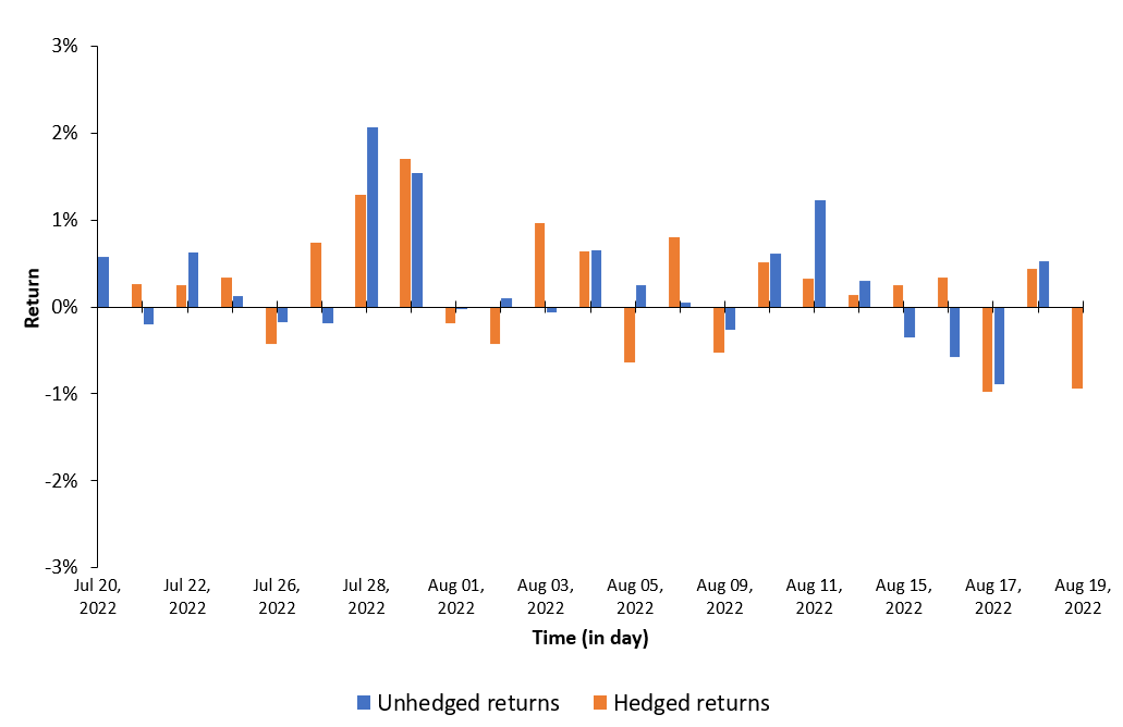
Hedged an unhedged return Source : computation by the author.

Currency overlay is a strategy that is implemented to manage currency exposures by hedging against foreign exchange risk. Currency overlay is typically used by institutional investors like big corporates, asset managers, pension funds, mutual funds, etc. For such investors exchange-rate risk is indeed a concern. Note that institutional investors often outsource the implementation of currency overlays to specialist financial firms (called “overlay managers”) with strong expertise in foreign exchange risk. The asset allocation and the foreign exchange risk management are then separated and done by two different persons (and entities), e.g., the asset manager and the overlay manager. This organization explains the origin of the world “overlay” as the foreign exchange risk management is a distinct layer in the management of the fund.

Overlay managers make use of derivatives like currency forwards, currency swaps, futures and options. The main idea is to offset the currency exposure embedded in the portfolio assets and providing hedged returns from the international securities. The implementation can include hedging all or a proportion of the currency exposure. Currency overlay strategies can be passive or active depending on portfolio-specific objectives, risk-appetite of investors and currency movement viewpoint.

Types of currency overlay strategies

Active currency overlay

Active currency overlay focuses on not just hedging the currency exposure, but also profiting additionally from exchange-rate movements. Investors keeps a part of their portfolio unhedged and take up speculative positions based on their viewpoint regarding the currency trends.

Passive currency overlay

A passive overlay focuses only on hedging the currency exposure to mitigate exchange-rate risk. Passive overlay is implemented through derivative contracts like currency forwards which are used to lock-in a specific exchange-rate for a fixed time-period, thus providing stability to asset values and protection against exchange-rate fluctuations.

Passive overlay is a simple strategy to implement and generally uses standardized contracts, however, it also eliminates the scope of generating any additional profits for the portfolio through exchange-rate fluctuations.

Implementing currency overlays

Base currency and benchmark

Base currency is generally the currency in which the portfolio is dominated or the investor’s domestic currency. A meaningful benchmark selection is also essential to analyze the performance and assess risk of the overlay. World market indices such as those published by MSCI, FTSE, S&P, etc. can be appropriate choices.

Hedge ratio

Establishing a strategic hedge ratio is a fundamental step in implementing a currency overlay strategy. It is the ratio of targeted exposure to be currency hedged by the overlay against the overall portfolio position. Different hedge ratios can have different impact on the portfolio returns and determining the optimal hedge ratio can depend on various factors such as investor risk-appetite and objectives, portfolio assets, benchmark selection, time horizon for hedging etc.

Cost of overlay

The focus of overlays is to hedge the fluctuations in foreign exchange rates by generating cashflows to offset the foreign exchange rate movements through derivatives like currency forwards, currency swaps, futures and options. The use of these derivatives products generates additional costs that impacts the overall performance of the portfolio strategy. These costs must be compared to the benefits of portfolio volatility reduction coming from the overlay implementation.

This cost is also an essential factor in the selection of the hedge ratio.

Note that passive overlays are generally cheaper than active overlays in terms of implementation costs.

Useful resources

Academic articles

Black, F. (1989) Optimising Currency Risk and Reward in International Equity Portfolios. Financial Analysts Journal, 45, 16-22.

Business material

Pensions and Lifetime Savings Association Currency overlay: why and how? video.

About the author

The article was written in September 2022 by Jayati WALIA (ESSEC Business School, Grande Ecole Program – Master in Management, 2019-2022).

My experience as a credit analyst at Amundi Asset Management

August 14, 2022 by Jayati WALIA

My experience as a credit analyst at Amundi Asset Management

In this article, Jayati WALIA (ESSEC Business School, Grande Ecole Program – Master in Management, 2019-2022) shares her apprenticeship experience as an assistant credit analyst in Amundi which is a leading European asset management firm.

About Amundi

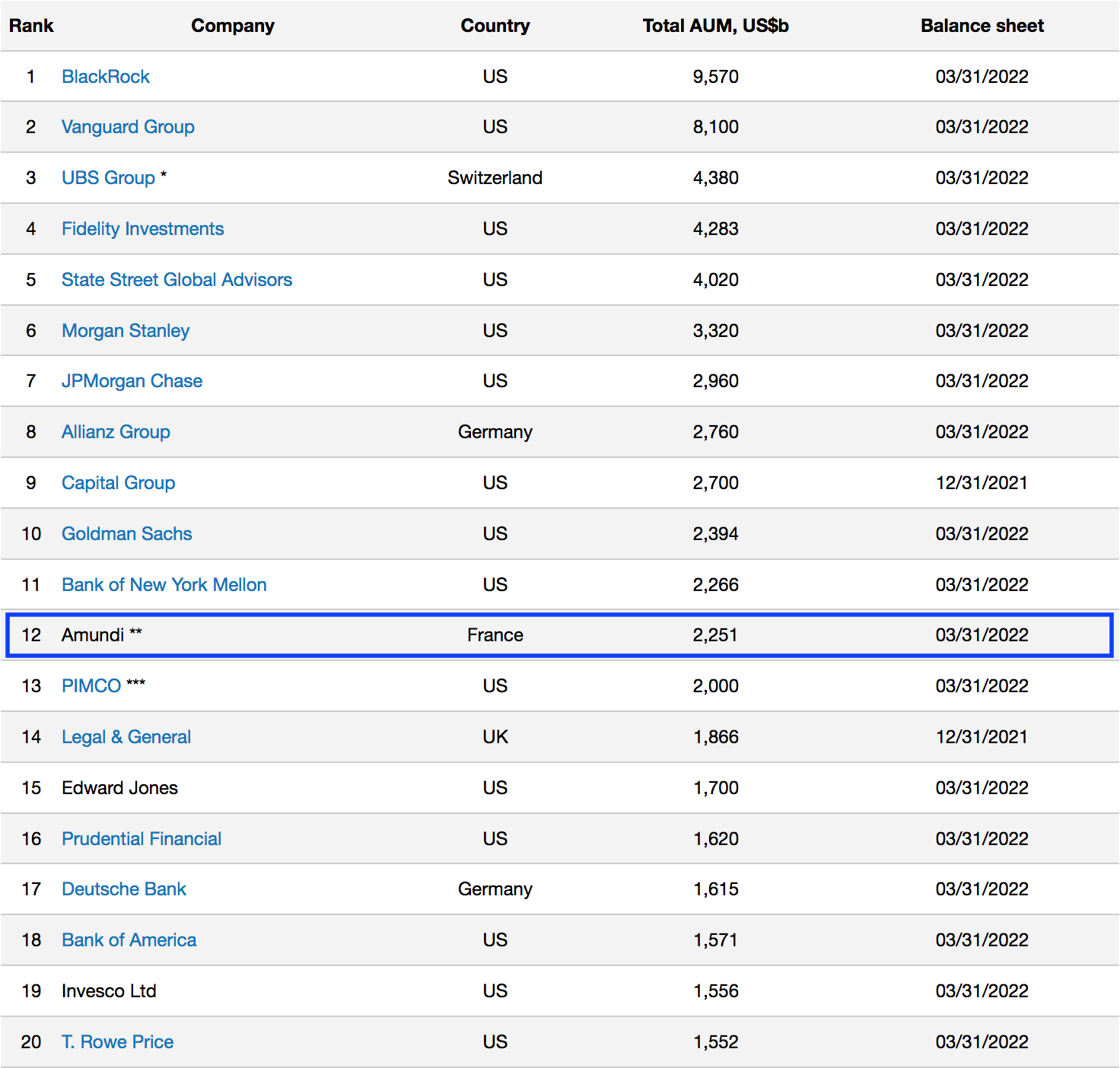
Amundi is a French asset management firm with currently over €2 trillion asset under management (AUM). It ranks among the top 15 asset managers in the world (see Table 1 below). Amundi is a public company quoted on Euronext with the highest market capitalization in Europe among asset management firms (€10.92 billion as of May 20, 2022). Amundi was founded in 2010 following a merger between Crédit Agricole Asset management and Société Générale Asset management.

Table 1. Rank of asset management firms by asset under management (AUM).
Top asset management firms rankings Source: www.advratings.com

Amundi has over 100 million clients (retail, institutional and corporate) and it offers a range of savings and investment solutions, services, advice, and technology in active and passive management, in both traditional and real assets.

Amundi logo Source: Amundi

My apprenticeship

My team at Amundi, Fixed Income Solutions, works in coordination with all the teams of the firm’s global bond management platform. The team’s work revolves majorly around product development on Amundi’s Fixed Income offerings including technological work, generating new investment ideas, and bringing them to clients both institutional and distributors. My position in the team is Assistant Credit Analyst.

Missions

My work primarily involves setting up tools and procedures linked to various investment solutions and portfolios handled by team. The tools are developed through algorithms in programming languages (mainly Python) and their functionalities range from analysis of market signals for investment, pricing of securities, risk monitoring and reporting. I worked on fixed-income portfolio construction and optimization algorithms implementing modern portfolio theory.

My daily responsibilities include report production related to daily fund activity such as monitoring fund balance and calculation of regulatory financial ratios to check for alignment against specific risk constraints. Additionally, I also participate in market research for new investment ideas through analysis of various fixed-income securities and derivatives.

Required skills and knowledge

The work and missions involved in my role require technical knowledge especially programming skills in Python, quantitative modelling and an understanding of financial markets, products and concepts of valuation, various types of risks and financial data analysis. Other behavioral skills such as project management, autonomy and interpersonal communication are also essential.

Three key financial concepts

The following are three key concepts that are used regularly in my work at Amundi:

Credit ratings

Credit ratings are extensively used in fixed income. They reflect the creditworthiness of a borrower entity such as a company or a government, which has issued financial debt instruments like loans and bonds.

Credit risk assessment for companies and governments is generally performed by rating agencies (such as S&P, Moody’s and Fitch) which analyze the internal and external, qualitative and quantitative attributes that drive the economic future of the entity.
Bonds can be grouped into the following categories based on their credit rating:

Investment grade bonds: These bonds are rated Baa3 (by Moody’s) or BBB- (by S&P and Fitch) or higher and have a low rate of default.
Speculative grade bonds: These bonds are rated Ba1 (by Moody’s) or BB+ (by S&P and Fitch) or lower and have a higher rate of default. They are thus riskier than investment grade bonds and issued at a higher yield. Speculative grade bonds are also referred to “high yield” and “junk bonds”.

Often, some bonds are designated “NR” (“not rated”) or “WR” (“withdrawn rating”) if no rating is available for them due to various reasons, such as lack of credible information.

Credit spreads

Credit spread essentially refers to the difference between the yields of a debt instrument (such as corporate bonds) and a benchmark (government or sovereign bond) with similar maturities but contrasting credit ratings. It is measured in basis points and is indictive of the premium of a risky investment over a risk-free one.

Credit spreads can tighten or widen over time depending on economic and market conditions. For instance, times of financial stress cause an increase in credit risk which leads to spread widening. Similarly, when markets rally, and credit risk is low, spreads tighten. Thus, credit spreads are an indicator of current macro-economic and market conditions.

Credit spreads are used by market participants for investment analysis and bond valuations.

Duration and convexity

Bond prices and interest rates share an inverse relationship, i.e., if interest rates go up, bond prices move down and similarly if interest rates go down, bond prices move up. Duration measures this price sensitivity of bonds with respect to interest rates and helps analyze interest-rate risk for bonds. Bonds with higher duration are more sensitive to interest rate changes and hence more volatile. Duration for a zero-coupon bond is equal to its time to maturity.

While duration is linear measure of bond price-interest rates relationship, in real life, the curve of bond prices against interest rates is convex i.e., the duration of the bonds also changes with change in interest-rates. Convexity measures this duration sensitivity of bonds with respect to interest rates.

Useful resources

Amundi

About the author

The article was written in August 2022 by Jayati WALIA (ESSEC Business School, Grande Ecole Program – Master in Management, 2019-2022).

Moving averages

August 7, 2022 by Jayati WALIA

Moving averages

In this article, Jayati WALIA (ESSEC Business School, Grande Ecole Program – Master in Management, 2019-2022) explains the concept of moving averages and its implementation in financial markets as an indicator in technical analysis of stock price movements.

What is a moving average?

A moving average is a technique to analyze a time-series of data points by taking subsets of data and computing their averages. The subsets of data can explicitly be of a fixed size like simple moving averages or implicitly take into account all past points like exponential moving averages. These averages computed on rolling windows constitute a new time series. The aim of this exercise is essentially to filter noise and smoothen out the data in order to identify an overall trend in the data.

In financial markets, moving averages are one of the most popular indicators used in technical analysis. A moving average is used to interpret the current trend of a stock price (or any asset). It basically shows the price fluctuations in a stock as a single curve and is calculated using previous prices. Hence, a moving average is a lagging indicator.

Moving averages can be computed for different time periods such as 10 days, 20 days or 200 days. The greater the length of the time period (the lag in the trend), the greater the degree of smoothness in the moving average, however, the lower the price sensitivity of the moving average.

To measure the direction and strength of a trend, moving averages involve price averaging to establish a baseline. For instance, if the price moves above the average, the indicated trend is bullish and if it moves below the average, the trend is bearish. Moving average crossovers are also used commonly in trading strategies to identify trends. It then involves two moving averages: one computed on a short-term period and another one computed over a long-term period. When a shorter period moving average crosses above a longer period moving average, the trend is identified as bullish and indicates a buy signal. When a shorter period moving average crosses below a longer period moving average, the trend is identified as bearish and indicates a sell signal.

Moving averages are also used in development of other indicators such as Bollinger’s bands and Moving Average Convergence Divergence (MACD).

Types of moving averages

The moving average indicator can be of many types. Two basic types of moving averages and their interpretation are explained below: simple moving average and exponential-weighted moving average.

Simple moving average

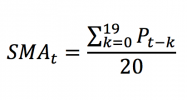
Simple moving average (SMA) is the easiest type of moving average to compute. An n-period SMA is simply calculated by taking the sum of the closing prices of an asset for the past ‘n’ time-periods divided by ‘n’.

The formula to compute the SMA at time t is given by:

Simple moving average formula

Where P_i represents the asset price at time i (i indicating any time between the interval [t-n, t]).

If the current asset price is greater than the SMA value, the viewpoint for trend is established as bullish and similarly, if the current asset price is less than the SMA value, the viewpoint for trend is established as bearish.

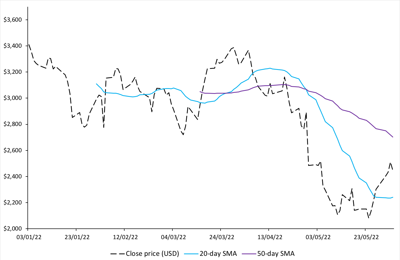
Figure 1 below illustrates the 20-day and 50-day SMA for Amazon stock price.

Figure 1. 20-day and 50-day simple moving averages for Amazon stock price.
20-day and 50-day SMA for Amazon stock price Source: Computation by author.

We can observe from the above figure that when the price is going down, the SMA also is going downwards (as expected from the formula). It can also be seen that the movement of the SMA curve lags the change in price movements. The greater is the chosen time-period for SMA, the greater is the lag observed. Thus, while a 50-day SMA maybe smoother compared to a 20-day SMA, the lag observed will also be greater.

Exponential-weighted moving average

Exponential-weighted moving average (EWMA), also known as exponential moving average (EMA) is an improvisation of moving average over the SMA. It assigns weights to moving averages such that the recent data points are assigned greater weight factors than older data points. Thus, EWMA is more sensitive to recent price changes and the line is smoother than that of SMA.

The formula to compute the value of the EWMA at time t is given by:

Exponential-weighted moving average formula

Where P_t represents the stock price at time t, and α is a smoothing (or weighting) factor.

The series is initialized as: EWMA₀ = P₀.

The smoothing factor, α, is a constant value which lies between 0 and 1. The higher the value of α, the greater the weight assigned to the recent data, and the less smooth the EWMA curve.

How to set alpha for an exponential-weighted moving average?

α can be varied by a trader using EWMA based on how heavily he or she wants the recent data to be weighted. If a single EWMA is being considered, an optimal value for alpha can be chosen by minimizing the mean-squared errors (MSE).

A rule of thumb sometimes by traders is specified as:
Alpha for EWMA

For instance, for a short-term EWMA with the lookback period, n = 20, and alpha is equal to 2/21 = 0.095. For a long-term EWMA with n = 50, and alpha is equal to 0.039. Note that n is not related to a meaningful number of days like for the SMA.

When α=2/(n+1), the weights of an SMA and EWMA have the same center of mass.

A more sophisticated method is to relate alpha to the ‘half-life’ concept, meaning how long it takes for the weight to become half of the weight of the most recent data.

If the formula of EWMA is expanded for k days, we get the following:

EWMA formula expanded

For α=2/(n+1), the idea is that for a sufficiently large value of n, the sum of weights assigned to last n days is around 86%.

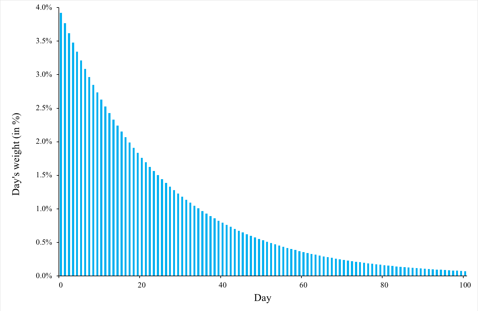
Figure 2 below illustrates the weights of each day for a EWMA with α equal to 3.92% (corresponding to n equal to 50 with the rule of thumb used by traders). It can be observed that the weights are decreasing in an exponential fashion and lower values are assigned as weights to the least recent days. The sum of the weights assigned to the first 10 days is 35.60 %, the first 50 days 86.47%, and the first 100 days 98.24%.

Figure 2. Weights of each day for an EWMA
EWMA day weights
Source: Computation by author.

Crossovers

EWMA is typically used in crossovers, which is a common strategy used by traders wherein two or more moving averages can help determine a more long-term trend. Basically, if a short-term EWMA crosses above a long-term EWMA, the crossover indicates an uptrend and similarly, if a short-term EWMA crosses below a long-term EWMA, the crossover indicates a downtrend. Traders can utilize it to establish their position in the stock.

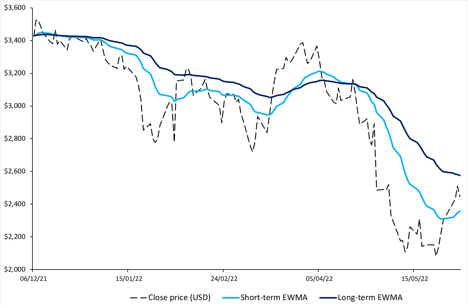
Figure 3. below illustrates short-term and long-term EWMA curves for Amazon stock prices.

Figure 3. Short-term and long-term EWMA for Amazon stock price.
img_SimTrade_EWMA_Amazon_stock
Source: Computation by author.

We can observe in the figure above that the short-term EWMA follows the price movements in Amazon stock more closely than the long-term EWMA does. We can also see that a crossover of the two EWMA curves is followed by a change in trend. For instance, in April 2022, the short-term EWMA crosses below the long-term EWMA and there is an evident downtrend observed post the crossover.

You can also download below the Excel file for computation of SMA and EWMA for Amazon stock price and visualize the above graphs.

Useful resources

Hunter, J. S. (1986). The exponentially weighted moving average. Journal of Quality Technology, 18:203–210.

Wikipedia Moving averages

National Institute of Standards and Technology (NIST) US Department of Commerce Single Exponential Smoothing

About the author

The article was written in August 2022 by Jayati WALIA (ESSEC Business School, Grande Ecole Program – Master in Management, 2019-2022).

Implied Volatility

May 15, 2022 by Jayati WALIA

In this article, Jayati WALIA (ESSEC Business School, Grande Ecole Program – Master in Management, 2019-2022) explains how implied volatility is computed from option market prices and a option pricing model.

Introduction

Volatility is a measure of fluctuations observed in an asset’s returns over a period of time. The standard deviation of historical asset returns is one of the measures of volatility. In option pricing models like the Black-Scholes-Merton model, volatility corresponds to the volatility of the underlying asset’s return. It is a key component of the model because it is not directly observed in the market and cannot be directly computed. Moreover, volatility has a strong impact on the option value.

Mathematically, in a reverse way, implied volatility is the volatility of the underlying asset which gives the theoretical value of an option (as computed by Black-Scholes-Merton model) equal to the market price of that option.

Implied volatility is a forward-looking measure because it is a representation of expected price movements in an underlying asset in the future.

Computation methods for implied volatility

The Black-Scholes-Merton (BSM) model provides an analytical formula for the price of both a call option and a put option.

The value for a call option at time t is given by:

Call option value

The value for a put option at time t is given by:

Put option value

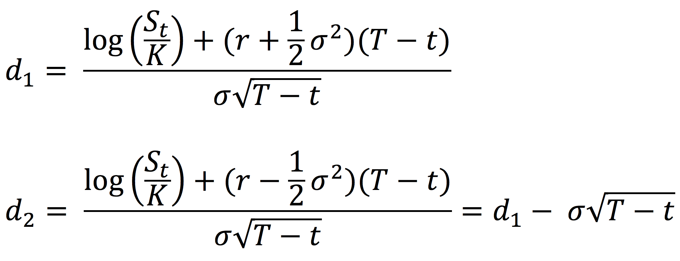
where the parameters d₁ and d₂ are given by:,

call option d1 d2

with the following notations:

S_t : Price of the underlying asset at time t
t: Current date
T: Expiry date of the option
K: Strike price of the option
r: Risk-free interest rate
σ: Volatility of the underlying asset
N(.): Cumulative distribution function for a normal (Gaussian) distribution. It is the probability that a random variable is less or equal to its input (i.e. d₁ and d₂) for a normal distribution. Thus, 0 ≤ N(.) ≤ 1

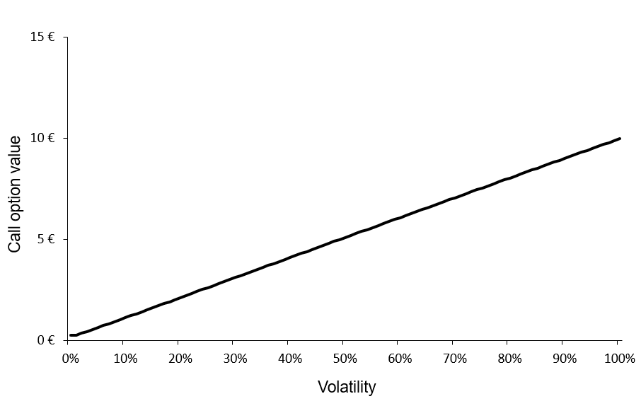
From the BSM model, both for a call option and a put option, the option price is an increasing function of the volatility of the underlying asset: an increase in volatility will cause an increase in the option price.

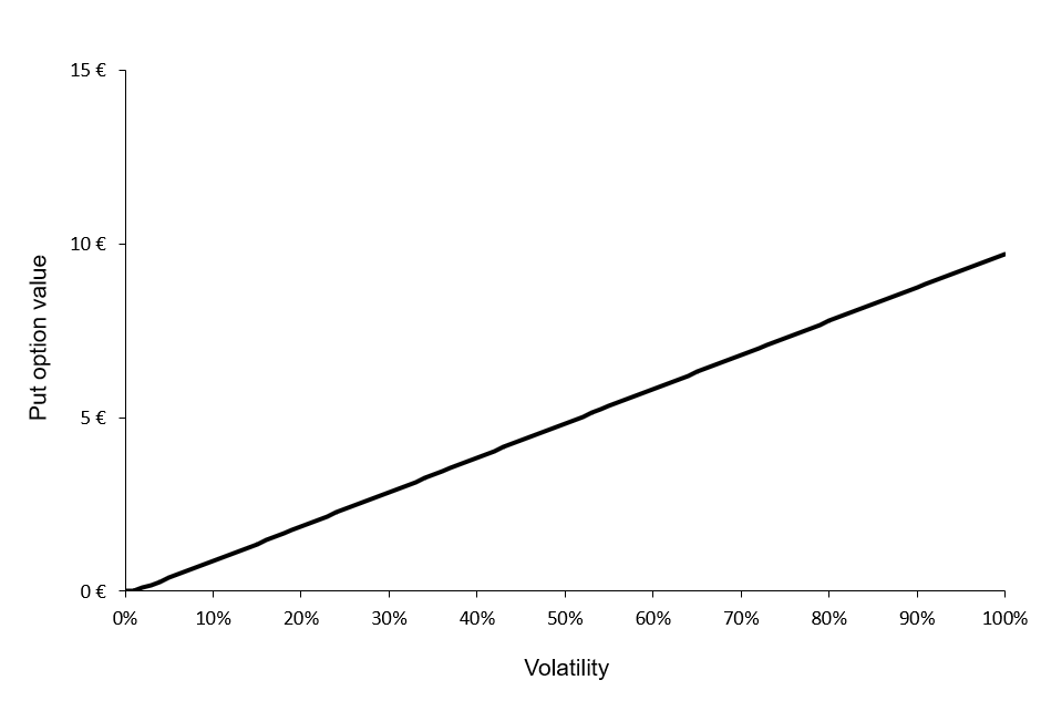
Figures 1 and 2 below illustrate the relationship between the value of a call option and a put option and the level of volatility of the underlying asset according to the BSM model.

Figure 1. Call option value as a function of volatility.

Source: computation by the author (BSM model)

Figure 2. Put option value as a function of volatility.

Source: computation by the author (BSM model)

You can download below the Excel file for the computation of the value of a call option and a put option for different levels of volatility of the underlying asset according to the BSM model.

We can observe that the call and put option values are a monotonically increasing function of the volatility of the underlying asset. Then, for a given level of volatility, there is a unique value for the call option and a unique value for the put option. This implies that this function can be reversed; for a given value for the call option, there is a unique level of volatility, and similarly, for a given value for the put option, there is a unique level of volatility.

The BSM formula can be reverse-engineered to compute the implied volatility i.e., if we have the market price of the option, the market price of the underlying asset, the market risk-free rate, and the characteristics of the option (the expiration date and strike price), we can obtain the implied volatility of the underlying asset by inverting the BSM formula.

Example

Consider a call option with a strike price of 50 € and a time to maturity of 0.25 years. The market risk-free interest rate is 2% and the current price of the underlying asset is 50 €. Thus, the call option is ‘at-the-money’. If the market price of the call option is equal to 2 €, then the associated level of volatility (implied volatility) is equal to 18.83%.

You can download below the Excel file below to compute the implied volatility given the market price of a call option. The computation uses the Excel solver.

Volatility smile

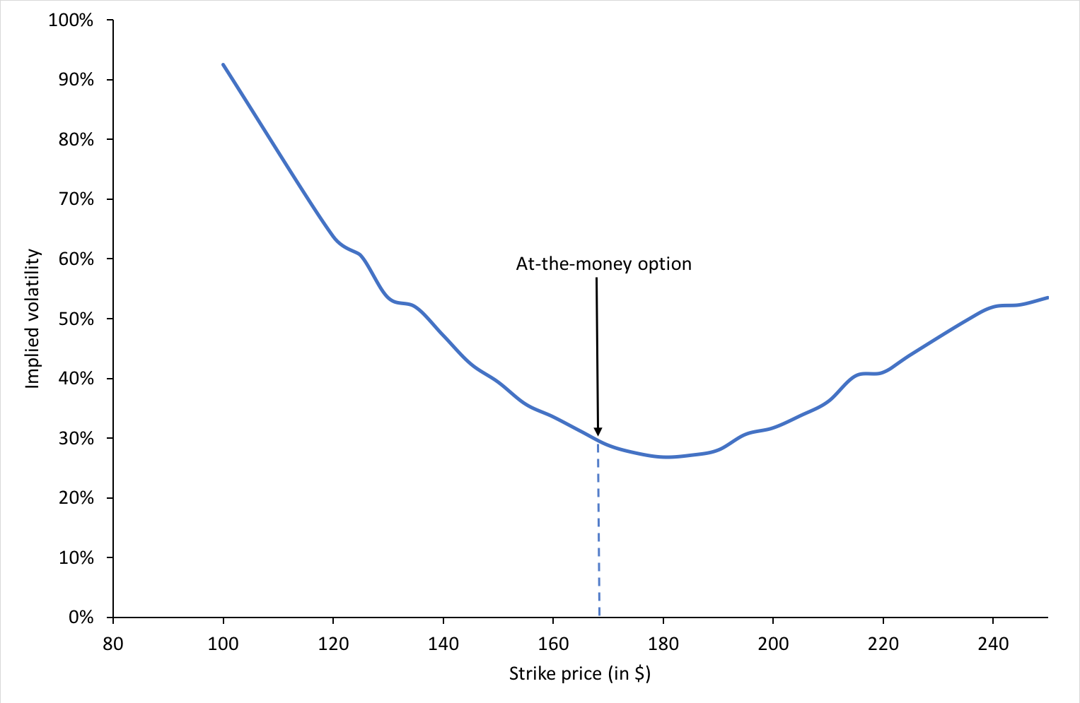
Volatility smile is the name given to the plot of implied volatility against different strikes for options with the same time to maturity. According to the BSM model, it is a horizontal straight line as the model assumes that the volatility is constant (it does not depend on the option strike). However, in practice, we do not observe a horizontal straight line. The curve may be in the shape of the alphabet ‘U’ or a ‘smile’ which is the usual term used to refer to the observed function of implied volatility.

Figure 3 below depicts the volatility smile for call options on the Apple stock on May 13, 2022.

Figure 3. Volatility smile for call options on Apple stock.
Apple volatility smile
Source: Computation by author.

We can also observe that the for a specific time to maturity, the implied volatility is minimum when the option is at-the-money.

Volatility surface

An essential assumption of the BSM model is that the returns of the underlying asset follow geometric Brownian motion (corresponding to log-normal distribution for the price at a given point in time) and the volatility of the underlying asset price remains constant over time until the expiration date. Thus theoretically, for a constant time to maturity, the plot of implied volatility and strike price would be a horizontal straight line corresponding to a constant value for volatility.

Volatility surface is obtained when values for implied volatilities are calculated for options with different strike prices and times to maturity.

CBOE Volatility Index

The Chicago Board Options Exchange publishes the renowned Volatility Index (also known as VIX) which is an index based on the implied volatility of 30-day option contracts on the S&P 500 index. It is also called the ‘fear gauge’ and it is a representation of the market outlook for volatility for the next 30 days.

Useful resources

Academic articles

Black F. and M. Scholes (1973) “The Pricing of Options and Corporate Liabilities” The Journal of Political Economy, 81, 637-654.

Dupire B. (1994). “Pricing with a Smile” Risk Magazine 7, 18-20.

Merton R.C. (1973) “Theory of Rational Option Pricing” Bell Journal of Economics, 4, 141–183.

Business

CBOE Volatility Index (VIX)

CBOE VIX tradable products

About the author

The article was written in May 2022 by Jayati WALIA (ESSEC Business School, Grande Ecole Program – Master in Management, 2019-2022).

Returns

April 20, 2022 by Jayati WALIA

In this article, Jayati WALIA (ESSEC Business School, Grande Ecole Program – Master in Management, 2019-2022) explains how returns of financial assets are computed and their interpretation in the world of finance.

Introduction

The main focus of any investment in financial markets is to make maximum profits within a coherent risk level. Returns in finance is a metric that inherently refers to the change in the value of any investment. Positive values of returns are interpreted as gains whereas negative values are interpreted as losses.

Returns are generally computed over standardized frequencies such as daily, monthly, yearly, etc. They can also be computed for specific time periods such as the holding period for ease of comparison and analysis.

Computation of returns

Consider an asset for a time period [t -1, t] with an initial price P_t-1 at time t-1 and final price P_t at time t (one period, two dates). Different forms of defining returns for the asset over period [t -1, t] are discussed below.

Arithmetic (percentage) returns

This is the simplest way for computation of returns.

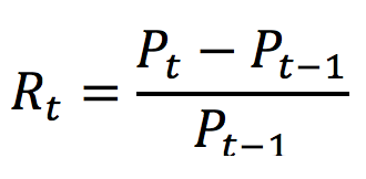
The return over the period [t -1, t], denoted by R_t, is expressed as:

Arithmetic returns

Logarithmic returns

Logarithmic returns (or log returns) are also used commonly to express investment returns. The log return over the period [t-1, t], denoted by R_t is expressed as:

Logarithmic returns

Log returns provide the property of time-additivity to the returns which essentially means that the log returns over a given period can be simply added together to compute the total return over subperiods. This feature is particularly useful in statistical analysis and reduction of algorithmic complexity.

Logarithmic returns additivity

Log returns are also known as continuously compounded returns because the rate of log returns is equivalent to the continuously compounding interest rate for the asset at price P₀ and time period t.

img_SimTrade_compounded_returns

Link between arithmetic and logarithmic returns

The arithmetic return (R^ari) and the logarithmic return (R^log) are linked by the following formula:

Relation between arithmetic and logarithmic returns

Components of total returns

The total return on an investment is essentially composed of two components: the yield and the capital gain (or loss). The yield refers to the periodic income or cash-flows that may be received on the investment. For example, for an investment in stocks, the yield corresponds to the revenues of dividends while for bonds, it corresponds to interest payments.

On the other hand, capital gain (or loss) refers to the appreciation (or depreciation) in the price of the investment. Thus, the capital gain (or loss) for any asset is essentially the price change in the asset.

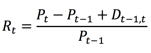
Total returns for a stock over the period [t -1, t], denoted by R_t, can hence be expressed as:

Total returns

Where
   P_t: Stock price at time t
   P_t-1: Stock price at time t-1
   D_t-1,t: Dividend obtained over the period [t -1, t]

Price changes and returns

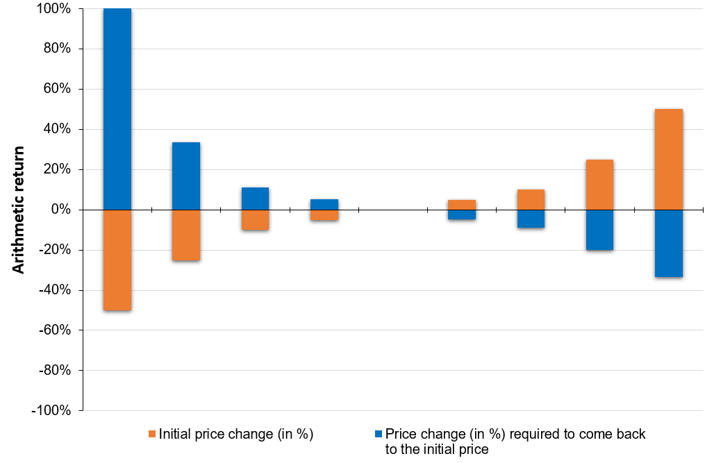
Consider a stock with an initial price of 100€ at time t=0. Suppose the stock price drops to 50€ at time t=1. Thus, there is a change of -50% (minus sign representing the decrease in price) in the initial stock price.

Now for the stock price to reach back to its initial price (100€ in this case) at time t=2 from its price of 50€ at time t=1, it will require an increase of (100€-50€)/50€ = 100%. With arithmetic returns, the increase (+100%) has to be higher than the decrease (-50%).

Similarly, for a price drop of -25% in the initial stock price of 100€, we would require an increase of 33% in the next time period to reach back the initial stock price. Figure 1 illustrates this asymmetry between positive and negative arithmetic returns.

Figure 1. Evolution of price change as a measure of arithmetic returns.
img_SimTrade_price_change_evolution
Source: computation by the author.

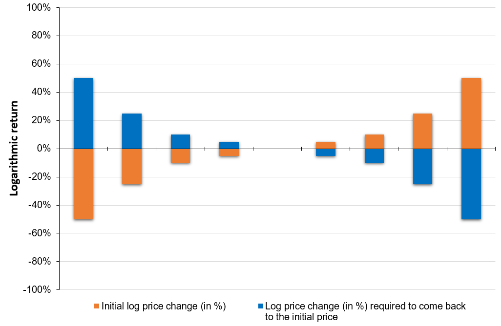
If the return is defined as a logarithmic return, there is a symmetry between positive and negative logarithmic returns as illustrated in Figure 2.

Figure 2. Evolution of price change as a measure of logarithmic returns.
img_SimTrade_price_change_evolution
Source: computation by the author.

You can also download below the Excel file for computation of arithmetic returns and visualise the above price change evolution.

Internal rate of return (IRR)

Internal rate of return (IRR) is the rate at which a project undertaken by the firm break’s even. It is a financial metric used by financial analysts to compute the profitability from an investment and is calculated by equating the initial investment and the discounted value of the future cashflows i.e., making the net present value (NPV) equal to zero. The IRR is the sprecail value of the discount rate which makes the NPV equal to zero.

The IRR for a project can be computed as follows:

IRR formula

Where,
CF_t : Cashflow for time period t

The higher the IRR from a project, the more desirable it is to pursue with the project.

Ex ante and ex post returns

Ex ante and ex post are Latin expressions. Ex ante refers to “before an event” while ex post refers to “after the event”. In context of financial returns, the ex ante return corresponds to prediction or estimation of an asset’s potential future return and can be based on a financial model like the Capital Asset Pricing Model (CAPM). On the other hand, the ex post return corresponds to the actual return generated by an asset historically, and hence are lagging or backward-looking in nature. Ex post returns can be used to forecast ex ante returns for the upcoming period and together, both are used to make sound investment decisions.

About the author

The article was written in April 2022 by Jayati WALIA (ESSEC Business School, Grande Ecole Program – Master in Management, 2019-2022).

The Monte Carlo simulation method for VaR calculation

January 30, 2024March 24, 2022 by Jayati WALIA

In this article, Jayati WALIA (ESSEC Business School, Grande Ecole – Master in Management, 2019-2022) explains the Monte Carlo simulation method for VaR calculation.

Introduction

Monte Carlo simulations are a broad class of computational algorithms that rely majorly on repeated random sampling to obtain numerical results. The underlying concept is to model the multiple possible outcomes of an uncertain event. It is a technique used to understand the impact of risk and uncertainty in prediction and forecasting models.

The Monte Carlo simulation method was invented by John von Neumann (Hungarian-American mathematician and computer scientist) and Stanislaw Ulam (Polish mathematician) during World War II to improve decision making under uncertain conditions. It is named after the popular gambling destination Monte Carlo, located in Monaco and home to many famous casinos. This is because the random outcomes in the Monte Carlo modeling technique can be compared to games like roulette, dice and slot machines. In his autobiography, ‘Adventures of a Mathematician’, Ulam mentions that the method was named in honor of his uncle, who was a gambler.

Calculating VaR using Monte Carlo simulations

The basic concept behind the Monte Carlo approach is to repeatedly run a large number of simulations of a random process for a variable of interest (such as asset returns in finance) covering a wide range of possible scenarios. These variables are drawn from pre-specified probability distributions that are assumed to be known, including the analytical function and its parameters. Thus, Monte Carlo simulations inherently try to recreate the distribution of the return of a position, from which VaR can be computed.

Consider the CAC40 index as our asset of interest for which we will compute the VaR using Monte Carlo simulations.

The first step in the simulation is choosing a stochastic model for the behavior of our random variable (the return on the CAC 40 index in our case).
A common model is the normal distribution; however, in this case, we can easily compute the VaR from the normal distribution itself. The Monte Carlo simulation approach is more relevant when the stochastic model is more complex or when the asset is more complex, leading to difficulties to compute the VaR. For example, if we assume that returns follow a GARCH process, the (unconditional) VaR has to be computed with the Monte Carlo simulation methods. Similarly, if we consider complex financial products like options, the VaR has to be computed with the Monte Carlo simulation methods.

In this post, we compare the Monte Carlo simulation method with the historical method and the variance-covariance method. Thus, we simulate returns for the CAC40 index using the GARCH (1,1) model.
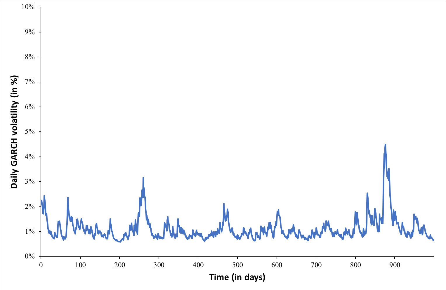
Figure 1 and 2 illustrate the GARCH simulated daily returns and volatility for the CAC40 index.

Figure 1. Simulated GARCH daily returns for the CAC40 index.
img_SimTrade_CAC40_GARCH_ret
Source: computation by the author.

Figure 2. Simulated GARCH daily volatility for the CAC40 index.
img_SimTrade_CAC40_GARCH_vol
Source: computation by the author.

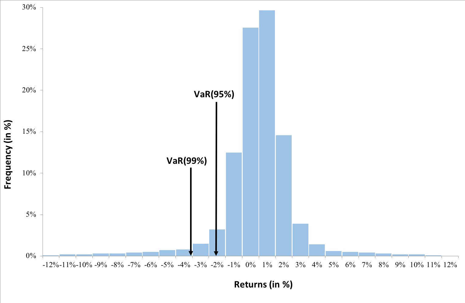
Next, we sort the distribution of simulated returns in ascending order (basically in order of worst to best returns observed over the period). We can now interpret the VaR for the CAC40 index in one-day time horizon based on a selected confidence level (probability).

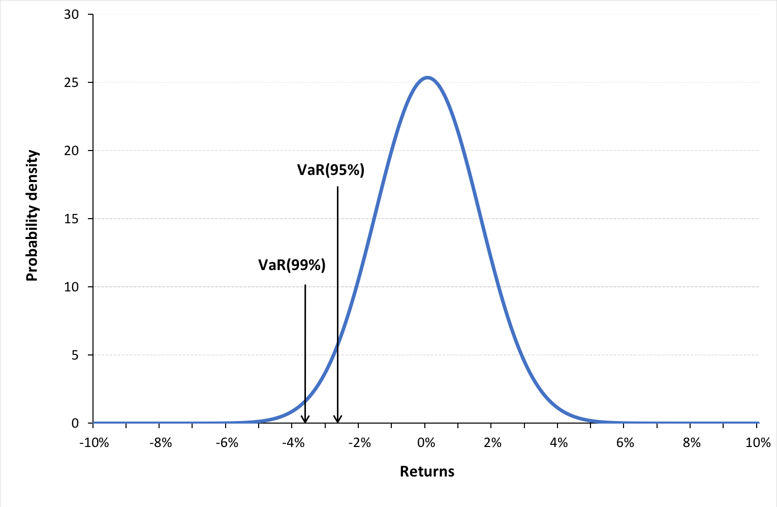
For instance, if we select a confidence level of 99%, then our VaR estimate corresponds to the 1st percentile of the probability distribution of daily returns (the bottom 1% of returns). In other words, there are 99% chances that we will not obtain a loss greater than our VaR estimate (for the 99% confidence level). Similarly, VaR for a 95% confidence level corresponds to bottom 5% of the returns.

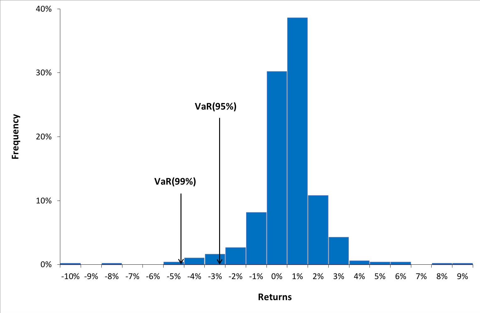
Figure 3 below represents the unconditional probability distribution of returns for the CAC40 index assuming a GARCH process for the returns.

Figure 3. Probability distribution of returns for the CAC40 index.
img_SimTrade_CAC40_MonteCarloVaR
Source: computation by the author.

From the above graph, we can interpret VaR for 99% confidence level as -3% i.e., there is a 99% probability that daily returns we obtain in future are greater than -3%. Similarly, VaR for 95% confidence level as -1.72% i.e., there is a 95% probability that daily returns we obtain in future are greater than -1.72%.

You can download below the Excel file for computation of VaR for CAC40 stock using Monte Carlo method involving GARCH(1,1) model for simulation of returns.

Advantages and limitations of Monte Carlo method for VaR

The Monte Carlo method is a very powerful approach to VAR due its flexibility. It can potentially account for a wide range of scenarios. The simulations also account for nonlinear exposures and complex pricing patterns. In principle, the simulations can be extended to longer time horizons, which is essential for risk measurement and to model more complex models of expected returns.

This approach, however, involves investments in intellectual and systems development. It also requires more computing power than simpler methods since the more is the number of simulations generated, the wider is the range of potential scenarios or outcomes modelled and hence, greater would be the potential accuracy of VaR estimate. In practical applications, VaR measures using Monte Carlo simulation often takes hours to run. Time requirements, however, are being reduced significantly by advances in computer software and faster valuation methods.

Useful resources

Jorion P. (2007) Value at Risk, Third Edition, Chapter 12 – Monte Carlo Methods, 321-326.

About the author

The article was written in March 2022 by Jayati WALIA (ESSEC Business School, Grande Ecole Program – Master in Management, 2019-2022).

Monte Carlo simulation method

March 17, 2022 by Jayati WALIA

In this article, Jayati WALIA (ESSEC Business School, Grande Ecole – Master in Management, 2019-2022) explains the Monte Carlo simulation method and its applications in finance.

Introduction

The Monte Carlo method was invented by John von Neumann (Hungarian-American mathematician and computer scientist) and Stanislaw Ulam (Polish mathematician) during World War II to improve decision making under uncertain conditions. It is named after the popular gambling destination Monte Carlo, located in Monaco and home to many famous casinos. This is because the random outcomes in the Monte Carlo modeling technique can be compared to games like roulette, dice and slot machines. In his autobiography, ‘Adventures of a Mathematician’, Ulam mentions that the method was named in honor of his uncle, who was a gambler.

How Monte Carlo simulation works

The main idea is to repeatedly run a large number of simulations of a random process for a variable of interest (such as an asset price in finance) covering a wide range of possible situations. The outcomes of this variables are drawn from a pre-specified probability distribution that is assumed to be known, including the analytical function and its parameters. Thus, Monte Carlo simulations inherently try to recreate the entire distribution of asset prices.

Example: Apple stock

Consider the Apple stock as our asset of interest for which we will generate stock prices according to the Monte Carlo simulation method.

The first step in the simulation is choosing a stochastic model for the behavior of our random variable (the Apple stock price in our case). A commonly used model is the geometric Brownian motion (GBM) model. The model assumes that future asset price changes are uncorrelated over time and the probability distribution function of the future price is a log-normal distribution. The movements in price in GBM process can be expressed as:

img_SimTrade_GBM_process

with dS being the change in asset price in continuous time dt. dW is the Wiener process (W_t+1 – W_t is a random variable from the normal distribution N(0, 1)). σ represents the price volatility considering the unexpected changes that can result from external effects (σ is assumed to be constant over time). μdt together represents the deterministic return within the time interval with μ representing the growth rate of the asset price or the ‘drift’.

Integrating dS/S over a finite interval, we get :

img_SimTrade_simulated_asset_price

Where ε is a random number generated from a normal distribution N(0,1).

This equation thus gives us the evolution of the asset price from a simulated model from day t-1 to day t.

We can now generate a simulation path for 100 days using the above formula.

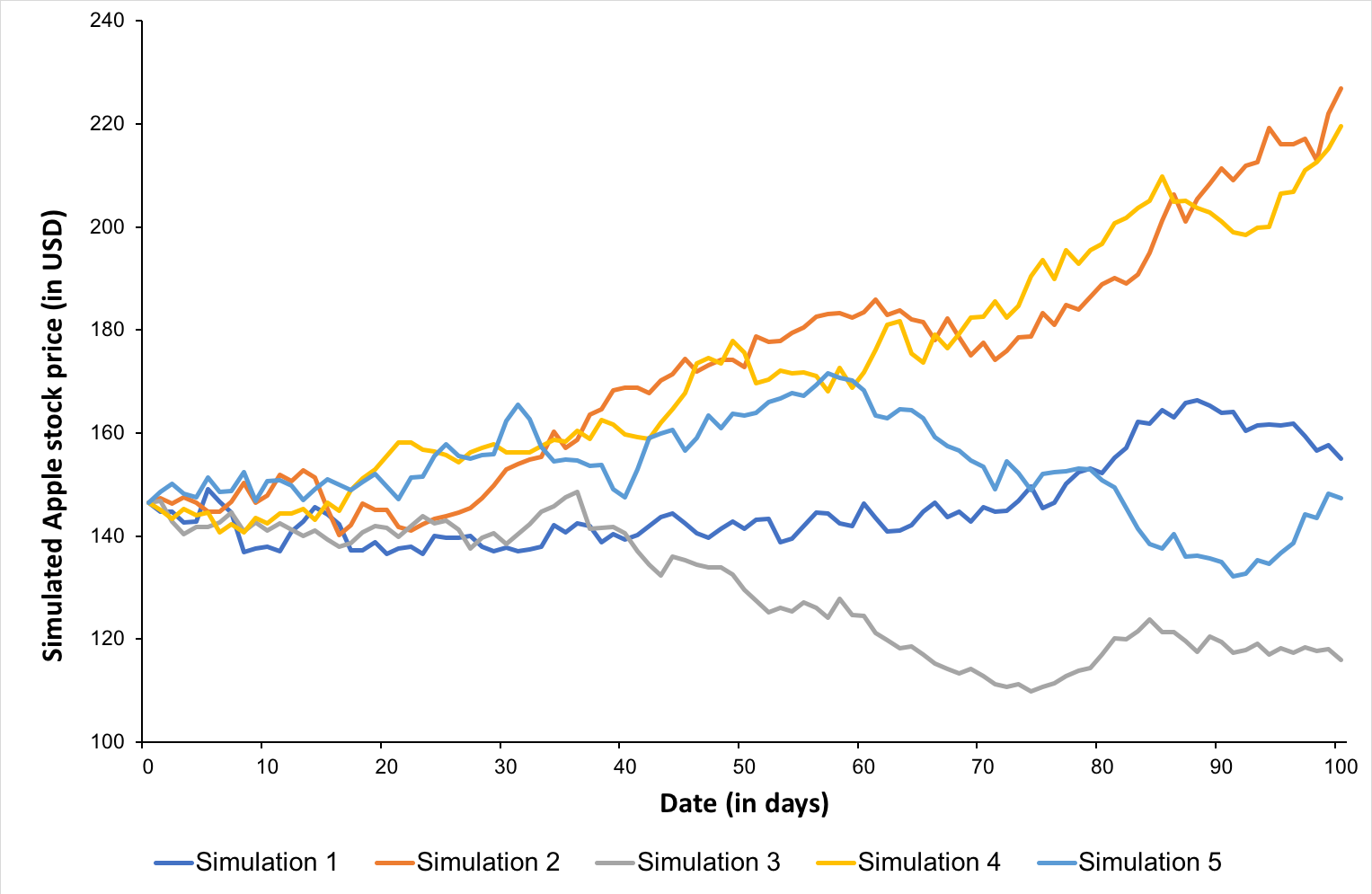
The figure below shows five simulations for the price of the Apple stock over 100 days with Δt = 1 day. The initial price for Apple stock (i.e, price at t=0) is $146.52.

Figure 1. Simulated Apple stock prices according to the Monte Carlo simulation method.
img_SimTrade_Apple_MonteCarloSim
Source: computation by author.

Thus, we can observe that the prices obtained by just these five simulations range from $100 to over $220.

You can download below the Excel file for generating Monte Carlo Simulations for Apple stock.

Applications in finance

The Monte Carlo simulation method is widely used in finance for valuation and risk analysis purposes.

One popular application is option pricing. For option contracts with complicated features (such as Asian options) or those with a combination of assets as their underlying, Monte Carlo simulations help generate multiple potential payoff scenarios for the option which are averaged out to determine the option price at the issuance date.

The Monte Carlo method is also used to assess potential risks by generating simulations of market variables affecting portfolios such as asset returns, interest rates, macroeconomic factors, etc. over different time periods. These simulations are then assessed as required for risk modelling and to compute risk metrics such as the value at Risk (VaR) of a position.

Other applications include personal finance planning and corporate project finance where simulations are generated to construct stochastic financial models for sensitivity analysis and net present value (NPV) projections.

Useful resources

Hull, J.(2008) Risk Management and Financial Institutions, Fifth Edition, Chapter 7 – Valuation and Scenario Analysis.

About the author

The article was written in March 2022 by Jayati WALIA (ESSEC Business School, Grande Ecole Program – Master in Management, 2019-2022).

Black-Scholes-Merton option pricing model

February 4, 2024March 3, 2022 by Jayati WALIA

In this article, Jayati WALIA (ESSEC Business School, Grande Ecole Program – Master in Management, 2019-2022) explains the Black-Scholes-Merton model to price options.

The Black-Scholes-Merton model (or the BSM model) is the world’s most popular option pricing model. Developed in the beginning of the 1970s, this model introduced to the world, a mathematical way of pricing options. Its success was essentially a starting point for new forms of financial derivatives in the knowledge that they could be priced accurately using the ideas and analyses pioneered by Black, Scholes and Merton and it set the foundation for the flourishing of modern quantitative finance. Myron Scholes and Robert Merton were awarded the Nobel Prize for their work on option pricing in 1997. Unfortunately, Fischer Black had died several years earlier but would certainly have been included in the prize had he been alive, and he was also listed as a contributor by Scholes and Merton.

Today, the Black-Scholes-Merton formula is widely used by traders in investment banks to price and hedge option contracts. Options are used by investors to hedge their portfolios to manage their risks.

Assumptions of the BSM Model

As any model, the BSM model relies on a set of assumptions:

The model considers European options, which we can only be exercised at their expiration date.
The price of the underlying asset follows a geometric Brownian motion (corresponding to log-normal distribution for the price at a given point in time).
The risk-free rate remains constant over time until the expiration date.
The volatility of the underlying asset price remains constant over time until the expiration date.
There are no dividend payments on the underlying asset.
There are no transaction costs on the underlying asset.
There are no arbitrage opportunities.

The BSM equation

The value of an option is a function of the price of the underlying stock and its statistical behavior over the life of the option.

A commonly used model is Geometric Brownian Motion (GBM). GBM assumes that future asset price differences are uncorrelated over time and the probability distribution function of the future prices is a log-normal distribution (or equivalently the probability distribution function of the future returns is a normal distribution). The price movements in a GBM process can be expressed as:

GBM equation

with dS being the change in the underlying asset price in continuous time dt and dX the random variable from the normal distribution (N(0, 1) or Wiener process). σ is the volatility of the underlying asset price (it is assumed to be constant). μdt represents the deterministic return within the time interval with μ representing the growth rate of asset price or the ‘drift’.

Therefore, option price is determined by these parameters that describe the process followed by the asset price over a period of time. The Black-Scholes-Merton equation governs the price evolution of European stock options in financial markets. It is a linear parabolic partial differential equation (PDE) and is expressed as:

BSM model equation

Where V is the value of the option (as a function of two variables: the price of the underlying asset S and time t), r is the risk-free interest rate (think of it as the interest rate which you would receive from a government debt or similar debt securities) and σ is the volatility of the log returns of the underlying security (say stocks).

The key idea behind the equation is to hedge the option and limit exposure to market risk posed by the asset. This is achieved by a strategy known as ‘delta hedging’ and it involves replicating the option through an equivalent portfolio with positions in the underlying asset and a risk-free asset in the right way so as to eliminate risk.

Thus, from the BSM equation we can derive the BSM formulae that describe the price of call and put options over their life time.

The BSM formulae

Note that the type of option we are valuing (call or put), the strike price and the maturity date do not appear in the above BSM equation. These elements only appear in the ‘final condition’ i.e., the option value at maturity, called the payoff function.

For a call option, the payoff C is given by:

C_T = max⁡(S_T – K; 0)

For a put option, the payoff is given by:

P_T = max⁡(K – S_T; 0)

The BSM formula is a solution to the BSM equation, given the boundary conditions (given by the payoff equations above). It calculates the price at time t for both a call and a put option.

The value for a call option at time t is given by:

Call option value equation

The value for a put option at time t is given by:

Put option value equation

where

With the notations:
S_t: Price of the underlying asset at time t
t: Current date
T: Expiry date of the option
K: Strike price of the option
r: Risk-free interest rate
σ: Volatility (the standard deviation of the return on the underlying asset)
N(.): Cumulative distribution function for a normal (Gaussian) distribution. It is the probability that a random variable is less or equal to its input (i.e. d₁ and d₂) for a normal distribution. Thus, 0 ≤ N(.) ≤ 1

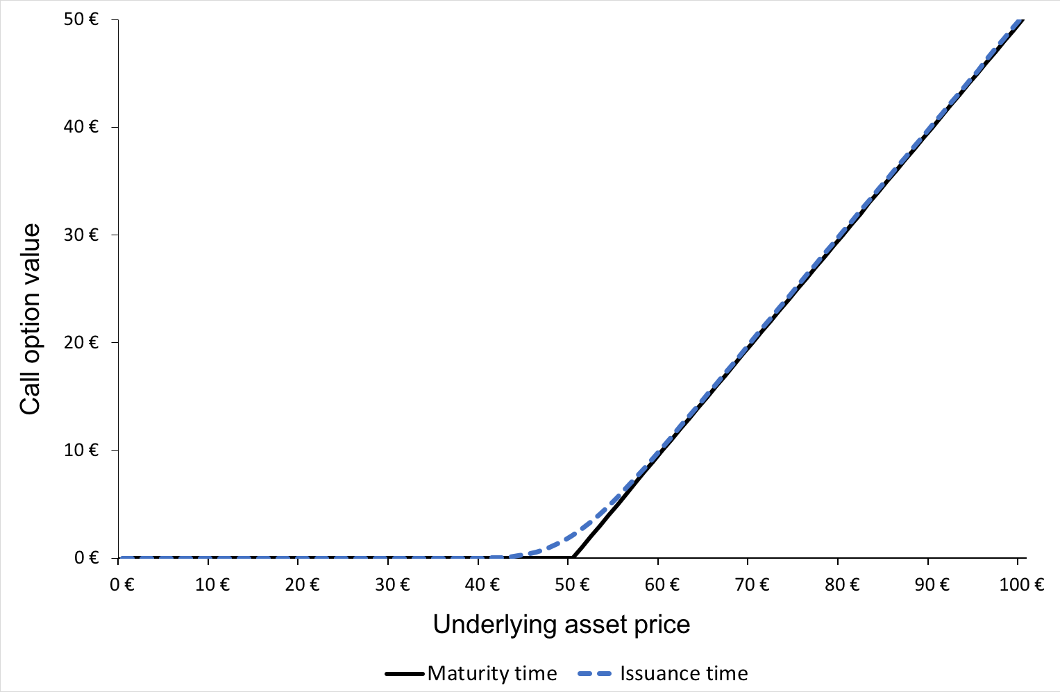
Figure 1 gives the graphical representation of the value of a call option at time t as a function of the price of the underlying asset at time t as given by the BSM formula. The strike price for the call option is 50€ with a maturity of 0.25 years and volatility of 50% in the underlying.

Figure 1. Call option value

Source: computation by author.

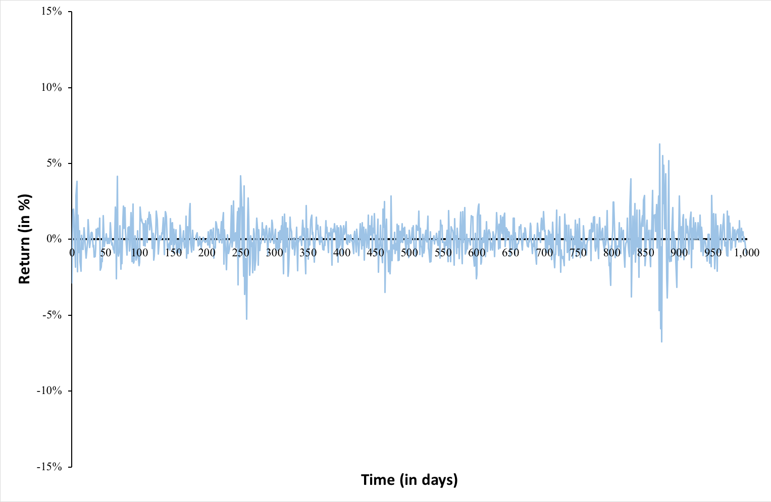
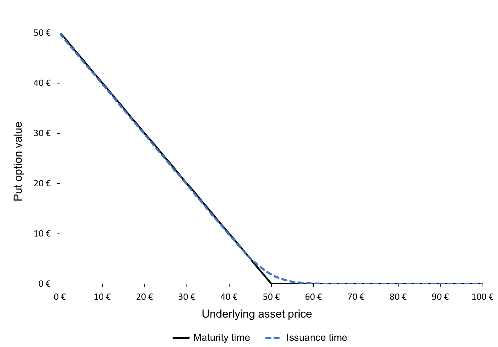
Figure 2 gives the graphical representation of the value of a put option at time t as a function of the price of the underlying asset at time t as given by the BSM formula. The strike price for the put option is 50€ with a maturity of 0.25 years and volatility of 50% in the underlying.

Figure 2. Put option value
Source: computation by author.

You can download below the Excel file for option pricing with the BSM Model.

Some Criticisms and Limitations

American options

The Black-Scholes-Merton model was initially developed for European options. This is a limitation of the equation for American options which can be exercised at any time before the expiry date. The BSM model would then not accurately determine the option value (an important case when the underlying asset pays a discrete dividend).

Stocks paying dividends

Also, in reality, most stocks pay dividends, and no dividends was an assumption in the initial BSM model, which analysts now eliminated by accommodating the dividend yield in the formula if required.

Constant volatility

Another limitation is the use of constant volatility. Volatility is the measure of risk based on the standard deviation of the return on the underlying asset. In reality the value of an asset will change randomly, not with a specific constant pattern regarding the way it can change.

Finally, the assumption of no transaction cost neglects the liquidity risk in the market since transaction costs are clearly incurred in the real world and there exists a bid-offer spread on most underlying assets. For the most heavily traded stocks, this cost may be low but for others it may lead to an inaccuracy.

Useful resources

Black F. and M. Scholes (1973) The Pricing of Options and Corporate Liabilities The Journal of Political Economy 81, 637-654.

Merton R.C. (1973) Theory of Rational Option Pricing Bell Journal of Economics 4, 141–183.

About the author

The article was written in March 2022 by Jayati WALIA (ESSEC Business School, Grande Ecole Program – Master in Management, 2019-2022).

Stress Testing used by Financial Institutions

January 16, 2022 by Jayati WALIA

Stress Testing used by Financial Institutions

In this article, Jayati WALIA (ESSEC Business School, Grande Ecole Program – Master in Management, 2019-2022) introduces the concept of Stress testing used by financial institutions to estimate the impact of extraordinary market conditions characterized by a high level of volatility like stock market crashes.

Introduction

Asset price movements in financial markets are based on several local or global factors which can include economic developments, risk aversion, asset-specific financial information amongst others. These movements may lead to adverse situations which can cause unpredicted losses to financial institutions. Since the financial crisis of 2008, the need for resilience of financial institutions against market shocks has been exemplified, and regulators around the world have implemented strict measures to ensure financial stability and stress testing has become an imperative part of those measures.

Stress testing techniques were applied in the 1990s by most large international banks. In 1996, the need for stress testing by financial institutions was highlighted by the Basel Committee on Banking Supervision (BCBS) in its regulation recommendations (Basel Capital Accord). Following the 2008 financial crisis, focus on stress testing to ensure adequate capital requirements was further enhanced under the Dodd-Frank Wall Street reform Act (2010) in the United States.

Financial institutions use stress testing as a tool to assess the susceptibility of their portfolios to potential adverse market conditions and protect the capital thus ensuring stability. Institutions create extreme scenarios based on historical, hypothetical, or simulated macro-economic and financial information to measure the potential losses on their investments. These scenarios can incorporate single market variable (such as asset prices or interest rates) or a group of risk factors (such as asset correlations and volatilities).

Thus, stress tests are done using statistical models to simulate returns based on portfolio behavior under exceptional circumstances that help in gauging the asset quality and different risks including market risk, credit risk and liquidity risk. By using the results of the stress tests, the institutions evaluate the quality of their processes and implement further controls or measures required to strengthen them. They can also be prepared to use different hedging strategies to mitigate the potential losses in case of an adverse event.

Types of Stress testing

Stress testing can be based on different sets of information incorporated in the tests. These sets of information can be of two types: historical stress testing and hypothetical stress testing.

Historical stress testing

In this approach, market risk factors are analyzed using historical information to run the stress tests which can include incorporating information from previous crisis episodes in order to measure potential losses the portfolio may incur in case a similar situation reoccurs. For example, the downfall in S&P500 (approximately 30% during February 2020-March 2020) due to the Covid pandemic could be used to gauge future downsides if any such event occurs again. A drawback of this approach is that historical returns alone may not provide sufficient information about the likelihood of abnormal but plausible market events.

The extreme value theory can be used for calculation of VaR especially for stress testing. considers the distribution of extreme returns instead of all returns i.e., extreme price movements observed during usual periods (which correspond to the normal functioning of markets) and during highly volatile periods (which correspond to financial crises). Thus, these extreme values cover almost all market conditions ranging from the usual environments to periods of financial crises which are the focus of stress testing.

Hypothetical stress testing

In this method, hypothetical scenarios are constructed in order to measure the vulnerability of portfolios to different risk factors. Simulation techniques are implemented to anticipate scenarios that may incur extreme losses for the portfolios. For example, institutions may run a stress test to determine the impact of a decline of 3% in the GDP (Gross Domestic Product) of a country on their fixed income portfolio based in that country. However, a drawback of this approach is estimating the likelihood of the generated hypothetical scenario since there is no evidence to back the possibility of it ever happening.

EBA Regulations

In order to ensure the disciplined functioning and stability of the financial system in the EU, the European Banking Authority (EBA) facilitates the EU-wide stress tests in cooperation with European Central Bank (ECB), the European Systemic Risk Board (ESRB), the European Commission (EC) and the Competent Authorities (CAs) from all relevant national jurisdictions. These stress tests are conducted every 2 years and include the largest banks supervised directly by the ECB. The scenarios, key assumptions and guidelines implemented in the stress tests are jointly developed by EBA, ESRB, ECB and the European Commission and the individual and aggregated results are published by the EBA.

The purpose of this EU-wide stress testing is to assess how well banks are able to cope with potentially adverse economic and financial shocks. The stress test results help to identify banks’ vulnerabilities and address them through informed supervisory decisions.

Useful resources

Wikipedia: Stress testing

EBA Guidelines: EU-wide stress testing

Longin F. (2000) From VaR to stress testing : the extreme value approach” Journal of Banking and Finance N°24, pp 1097-1130.

▶ Walia J. Quantitative Risk Management

▶ Walia J. Value at Risk

▶ Walia J. The historical method for VaR calculation

▶ Walia J. The variance-covariance method for VaR calculation

About the author

Article written in January 2022 by Jayati Walia (ESSEC Business School, Master in Management, 2019-2022).

The historical method for VaR calculation

January 30, 2024December 17, 2021 by Jayati WALIA

In this article, Jayati WALIA (ESSEC Business School, Grande Ecole Program – Master in Management, 2019-2022) presents the historical method for VaR calculation.

Introduction

A key factor that forms the backbone for risk management is the measure of those potential losses that an institution is exposed to any investment. Various risk measures are used for this purpose and Value at Risk (VaR) is the most commonly used risk measure to quantify the level of risk and implement risk management.

VaR is typically defined as the maximum loss which should not be exceeded during a specific time period with a given probability level (or ‘confidence level’). VaR is used extensively to determine the level of risk exposure of an investment, portfolio or firm and calculate the extent of potential losses. Thus, VaR attempts to measure the risk of unexpected changes in prices (or return rates) within a given period. Mathematically, the VaR corresponds to the quantile of the distribution of returns.

The two key elements of VaR are a fixed period of time (say one or ten days) over which risk is assessed and a confidence level which is essentially the probability of the occurrence of loss-causing event (say 95% or 99%). There are various methods used to compute the VaR. In this post, we discuss in detail the historical method which is a popular way of estimating VaR.

Calculating VaR using the historical method

Historical VaR is a non-parametric method of VaR calculation. This methodology is based on the approach that the pattern of historical returns is indicative of the pattern of future returns.

The first step is to collect data on movements in market variables (such as equity prices, interest rates, commodity prices, etc.) over a long time period. Consider the daily price movements for CAC40 index within the past 2 years (512 trading days). We thus have 512 scenarios or cases that will act as our guide for future performance of the index i.e., the past 512 days will be representative of what will happen tomorrow.

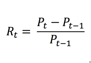
For each day, we calculate the percentage change in price for the CAC40 index that defines our probability distribution for daily gains or losses. We can express the daily rate of returns for the index as:
img_historicalVaR_returns_formula

Where R_t represents the (arithmetic) return over the period [t-1, t] and P_t the price at time t (the closing price for daily data). Note that the logarithmic return is sometimes used (see my post on Returns).

Next, we sort the distribution of historical returns in ascending order (basically in order of worst to best returns observed over the period). We can now interpret the VaR for the CAC40 index in one-day time horizon based on a selected confidence level (probability).

Since the historical VaR is estimated directly from data without estimating or assuming any other parameters, hence it is a non-parametric method.

For instance, if we select a confidence level of 99%, then our VaR estimate corresponds to the 1st percentile of the probability distribution of daily returns (the top 1% of worst returns). In other words, there are 99% chances that we will not obtain a loss greater than our VaR estimate (for the 99% confidence level). Similarly, VaR for a 95% confidence level corresponds to top 5% of the worst returns.

Figure 1. Probability distribution of returns for the CAC40 index.
Historical method VaR
Source: computation by the author (data source: Bloomberg).

You can download below the Excel file for the VaR calculation with the historical method. The historical distribution is estimated with historical data from the CAC 40 index.

From the above graph, we can interpret VaR for 90% confidence level as -3.99% i.e., there is a 90% probability that daily returns we obtain in future are greater than -3.99%. Similarly, VaR for 99% confidence level as -5.60% i.e., there is a 99% probability that daily returns we obtain in future are greater than -5.60%.

Advantages and limitations of the historical method

The historical method is a simple and fast method to calculate VaR. For a portfolio, it eliminates the need to estimate the variance-covariance matrix and simplifies the computations especially in cases of portfolios with a large number of assets. This method is also intuitive. VaR corresponds to a large loss sustained over an historical period that is known. Hence users can go back in time and explain the circumstances behind the VaR measure.

On the other hand, the historical method has a few of drawbacks. The assumption is that the past represents the immediate future is highly unlikely in the real world. Also, if the horizon window omits important events (like stock market booms and crashes), the distribution will not be well represented. Its calculation is only as strong as the number of correct data points measured that fully represent changing market dynamics even capturing crisis events that may have occurred such as the Covid-19 crisis in 2020 or the financial crisis in 2008. In fact, even if the data does capture all possible historical dynamics, it may not be sufficient because market will never entirely replicate past movements. Finally, the method assumes that the distribution is stationary. In practice, there may be significant and predictable time variation in risk.

Useful resources

Jorion, P. (2007) Value at Risk , Third Edition, Chapter 10 – VaR Methods, 276-279.

Longin F. (2000) From VaR to stress testing : the extreme value approach Journal of Banking and Finance, 24, 1097-1130.

About the author

The article was written in December 2021 by Jayati WALIA (ESSEC Business School, Grande Ecole Program – Master in Management, 2019-2022).

The variance-covariance method for VaR calculation

January 30, 2024December 17, 2021 by Jayati WALIA

In this article, Jayati WALIA (ESSEC Business School, Grande Ecole – Master in Management, 2019-2022) presents the variance-covariance method for VaR calculation.

Introduction

The two key elements of VaR are a fixed period of time (say one or ten days) over which risk is assessed and a confidence level which is essentially the probability of the occurrence of loss-causing event (say 95% or 99%). There are various methods used to compute the VaR. In this post, we discuss in detail the variance-covariance method for computing value at risk which is a parametric method of VaR calculation.

Assumptions

The variance-covariance method uses the variances and covariances of assets for VaR calculation and is hence a parametric method as it depends on the parameters of the probability distribution of price changes or returns.

The variance-covariance method assumes that asset returns are normally distributed around the mean of the bell-shaped probability distribution. Assets may have tendency to move up and down together or against each other. This method assumes that the standard deviation of asset returns and the correlations between asset returns are constant over time.

VaR for single asset

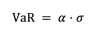
VaR calculation for a single asset is straightforward. From the distribution of returns calculated from daily price series, the standard deviation (σ) under a certain time horizon is estimated. The daily VaR is simply a function of the standard deviation and the desired confidence level and can be expressed as:

img_VaR_single_asset

Where the parameter ɑ links the quantile of the normal distribution and the standard deviation: ɑ = 2.33 for p = 99% and ɑ = 1.645 for p = 90%.

In practice, the variance (and then the standard deviation) is estimated from historical data.
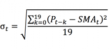
img_VaR_asset_variance

Where R_t is the return on period [t-1, t] and R the average return.

Figure 1. Normal distribution for VaR for the CAC40 index
Normal distribution VaR for the CAC40 index
Source: computation by the author (data source: Bloomberg).

You can download below the Excel file for the VaR calculation with the variance-covariance method. The two parameters of the normal distribution (the mean and standard deviation) are estimated with historical data from the CAC 40 index.

VaR for a portfolio of assets

Consider a portfolio P with N assets. The first step is to compute the variance-covariance matrix. The variance of returns for asset X can be expressed as:

Variance

To measure how assets vary with each other, we calculate the covariance. The covariance between returns of two assets X and Y can be expressed as:

Covariance

Where X_t and Y_t are returns for asset X and Y on period [t-1, t].

Next, we compute the correlation coefficients as:

img_correlation_coefficient

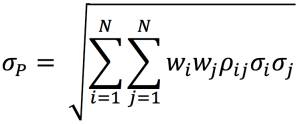
We calculation the standard deviation of portfolio P with the following formula:

img_VaR_std_dev_portfolio

img_VaR_std_dev_portfolio_2

Where w_i corresponds to portfolio weights of asset i.

Now we can estimate the VaR of our portfolio as:

img_portfolio_VaR

Where the parameter ɑ links the quantile of the normal distribution and the standard deviation: ɑ = 2.33 for p = 99% and ɑ = 1.65 for p = 95%.

Advantages and limitations of the variance-covariance method

Investors can estimate the probable loss value of their portfolios for different holding time periods and confidence levels. The variance–covariance approach helps us measure portfolio risk if returns are assumed to be distributed normally. However, the assumptions of return normality and constant covariances and correlations between assets in the portfolio may not hold true in real life.

Useful resources

Jorion P. (2007) Value at Risk, Third Edition, Chapter 10 – VaR Methods, 274-276.

About the author

The article was written in December 2021 by Jayati WALIA (ESSEC Business School, Grande Ecole Program – Master in Management, 2019-2022).

Standard deviation

December 9, 2021 by Jayati WALIA

Standard deviation

In this article, Jayati WALIA (ESSEC Business School, Grande Ecole Program – Master in Management, 2019-2022) presents an overview of standard deviation and its use in financial markets.

Mathematical formulae

To identify the center or average of any data set, measures of central tendency such as mean, median, mode and so on are used. These measures can be inherently used to represent any typical value in the particular data set. Considering a variable X, the arithmetic mean of a data set with N observations, X₁, X₂ … X_N, is computed as:

img_arithmetic_mean

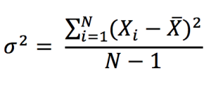
In the data set analysis, we also consider the dispersion or variability of data values around the central tendency or the mean. The variance of a data set is a measure of dispersion of data set values from the (estimated) mean and can be expressed as:

variance

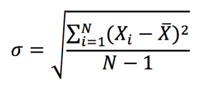
A problem with variance, however, is the difficulty of interpreting it due to its squared unit of measurement. This issue is resolved by using the standard deviation, which has the same measurement unit as the observations of the data set (such as percentage, dollar, etc.). The standard deviation is computed as the square root of variance:

standard deviation

A low value standard deviation indicates that the data set values tend to be closer to the mean of the set and thus lower dispersion, while a high standard deviation indicates that the values are spread out over a wider range indication higher dispersion.

Measure of volatility

For financial investments, the X variable in the above formulas would correspond to the return on the investment computed on a given period of time. We usually consider the trade-off between risk and reward. In this context, the reward corresponds to the expected return measured by the mean, and the risk corresponds to the standard deviation of returns.

In financial markets, the standard deviation of asset returns is used as a statistical measure of the risk associated with price fluctuations of any particular security or asset (such as stocks, bonds, etc.) or the risk of a portfolio of assets (such as mutual funds, index mutual funds or ETFs, etc.).

Investors always consider a mathematical basis to make investment decisions known as mean-variance optimization which enables them to make a meaningful comparison between the expected return and risk associated with any security. In other words, investors expect higher future returns on an investment on average if that investment holds a relatively higher level of risk or uncertainty. Standard deviation thus provides a quantified estimate of the risk or volatility of future returns.

In the context of financial securities, the higher the standard deviation, the greater is the dispersion between each return and the mean, which indicates a wider price range and hence greater volatility. Similarly, the lower the standard deviation, the lesser is the dispersion between each return and the mean, which indicates a narrower price range and hence lower volatility for the security.

Example: Apple Stock

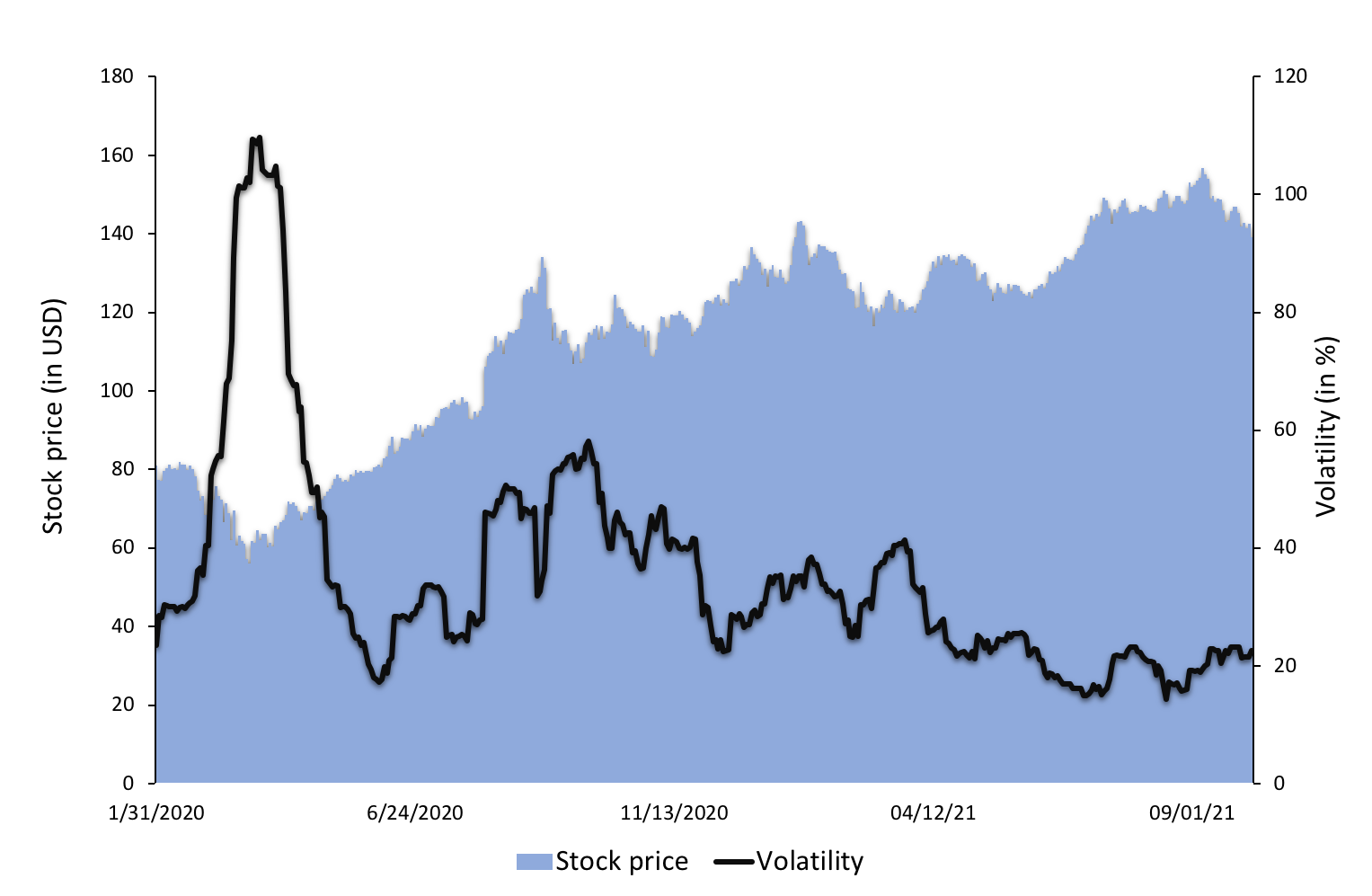
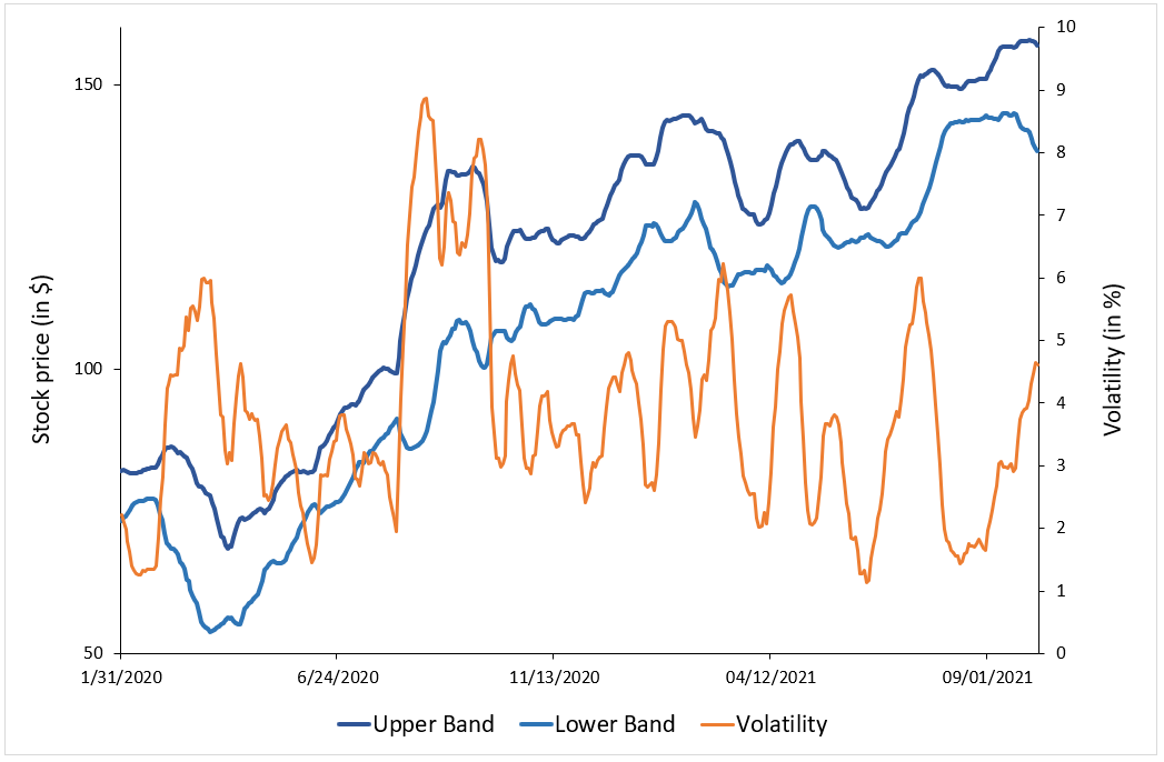
To illustrate the concept of volatility in financial markets, we use a data set of Apple stock prices. At each date, we compute the volatility as the standard deviation of daily stock returns over a rolling window corresponding to the past calendar month (about 22 trading days). This daily volatility is then annualized and expressed as a percentage.

Figure 1. Stock price and volatility of Apple stock.

price and volatility for Apple stock
Source: computation by the author (data source: Bloomberg).

You can download below the Excel file for the calculation of the volatility of stock returns. The data used are for Apple for the period 2020-2021.

Useful resources

Wikipedia Standard Deviation

About the author

The article was written in November 2021 by Jayati WALIA (ESSEC Business School, Grande Ecole Program – Master in Management, 2019-2022).

Logistic Regression

December 9, 2021 by Jayati WALIA

In this article, Jayati WALIA (ESSEC Business School, Grande Ecole – Master in Management, 2019-2022) presents an overview of logistic regression and its application in finance.

Introduction

Logistic regression is a predictive analysis regression method that is used in classification to determine whether an output that is categorical, belongs to a particular class or category. Mathematically, this means that the dependent variable in regression is dichotomous or binary i.e., it can take the values 0 or 1. Logistic regression is used to describe data and explain the relationship between one dependent binary variable and one or more nominal, ordinal, interval or ratio-level independent variables.

For instance, consider a weather forecasting situation. If we wish to predict the likelihood of whether it will rain or not on a particular day, linear regression is not going to be of use in this scenario because our outcome or value of dependent variable is unbounded. On the other hand, a binary logistic regression model will provide with a classified outcome (1: it will rain; 0: it will not rain).

Logistic regression analysis is valuable for predicting the likelihood of an event. It helps determine the probabilities between any two classes. In essence, logistic regression helps solve probability and classification problems.

Logistic Function

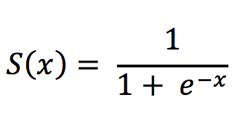
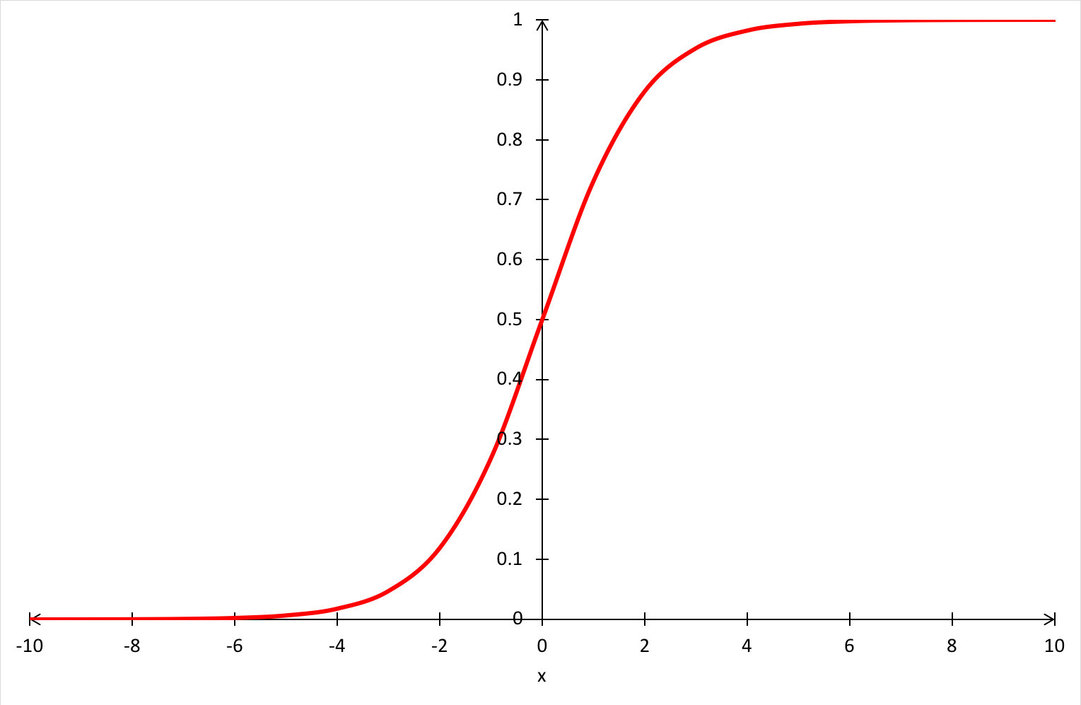
Logistic regression model uses the sigmoid function to map the output of a linear equation between 0 and 1. The sigmoid function is an S-shaped curve and can be expressed as:

sigmoid function

Figure 1. Sigmoid function curve.

img_sigmoid_function_curve

Source: computation by the author.

For logistic regression, we initially model the relationship between the dependent and independent variables as a linear equation as follows:

linear equation for logistic regression

wherein Y is the dependent variable (i.e., the variable we want to predict) and X is the explanatory variables (i.e., the variables we use to predict the dependent variable). β₀, β₁, β₂… β_N are regression coefficients that are generally estimated using the maximum likelihood estimation method.

This equation is mapped to the sigmoid function to squeeze the value of the outcome (Y) from a large scale to within the range 0 – 1. We get our logistic regression equation as:

logistic regression equation

The dependent variable Y is assumed to follow a Bernoulli distribution with parameter p defined as p = Probability(Y = 1). Thus, the main use-case of a logistic model is that with given observations of the variables (X₁,X₂ …, X_N) we estimate the probability p that the outcome Y is equal to 1.

Note that the logistic regression model is sensitive to outliers and the number of explanatory variables should be less than the total observations to avoid overfitting. The logistic regression model is generally combined with artificial neural networks to make it more suitable to assess complex relationships. In practice, it is performed using programming languages like Python and R which possess powerful libraries (packages) to evaluate the models.

Applications

Logistic regression is a relatively simple and efficient method for binary classification problems. It is a classification model that achieves very good performance with linearly separable classes or categories and is extensively employed in various industries such as medicine, gaming, hospitality, retail, etc.

In finance, the logistic regression model is commonly used to model the credit risk of individuals and small and medium enterprises. For companies, this model is used to predict their bankruptcy probability. Such a method is called credit scoring. To construct a logistic regression model for credit scoring of corporate firms, the independent variables are usually financial ratios computed with the information contained in financial statements: EBIT margin, return on equity (RoE), debt to equity (D/E), liquidity ratio, EBIT/Total Assets, etc. Further predictive statistical metrics like p-value and correlation test for multicollinearity can be used to narrow down to the variables with most contribution to the model.

Useful resources

Wikipedia Maximum Likelihood Estimation

Towards Data Science Logistic Regression

About the author

The article was written in November 2021 by Jayati WALIA (ESSEC Business School, Grande Ecole Program – Master in Management, 2019-2022).

Bollinger Bands

November 18, 2021 by Jayati WALIA

Bollinger Bands

In this article, Jayati WALIA (ESSEC Business School, Grande Ecole Program – Master in Management, 2019-2022) presents the popular Bollinger bands used in technical analysis.

This post is organized as follows: we introduce the concept of Bollinger bands and provide an illustration with Apple stock prices. We delve into the interpretation of Bollinger bands as port and resistance price levels used to define buy and sell trading signals. We then present the techniques to compute the Bollinger bands and finally discuss their limitations.

Introduction

In the 1980s, John Bollinger, a long-time market technical analyst, developed a technical analysis tool for trading in securities. At that time, it was presumed that volatility was a static quantity, a property of a security, and if it changed at all, it would happen in a long-term period. After some experimentation, Bollinger figured that volatility was indeed a very dynamic quantity and a moving average computed on a time period (typically 20 days) with bands drawn above and below at intervals could be determined by a multiple of standard deviation.

Unlike a percentage calculation from a simple moving average, Bollinger bands simply add and subtract a standard deviation (or a multiple of the standard deviation, usually two). The tool thus represents the volatility in the prices of the security which is measured by the standard deviation of the prices of the security. The bands are used to understand the overbought or oversold levels for a security and to follow the price trends. The indicator/tool comprises of three main bands, an upper band, a lower band, and a middle band.

The middle band is a simple moving average (SMA), which is usually computed over a rolling period of 20 trading days (about a calendar month). The upper and the lower bands are positioned two standard deviations away from the SMA. The change in the distance of the upper and lower bands from the SMA determine the price strength (which is the strength of price trend of stock relative to overall market trend) and the lower and the upper levels for the stock prices. Bollinger bands can be applied to all financial securities traded in the market including equities, forex, commodities, futures, etc. They are used in multiple time frames (daily, weekly and monthly) and can be even applied to very short-term periods such as hours.

Figure 1 represents the evolution of the price of Apple stocks with the Bollinger bands for the period January 2020 – September 2021.

Figure 1. Bollinger bands on Apple stock.
Bollinger bands Apple stock
Source: computation by the author (data source: Bloomberg).

Figure 2 illustrates for the price of Apple stocks the link between the Bollinger bands and volatility measured by the standard deviation of prices. The lower the volatility, the narrower the bands.

Figure 2. Bollinger’s bands and volatility
Bollinger bands and volatility Apple stock
Source: computation by the author (data source: Bloomberg).

How to interpret Bollinger bands

Traders use the Bollinger bands to determine the strength of the price trend of a stock. The upper and lower bands measure the degree of volatility in prices over time. The width between the bands widens as the volatility in the stock prices increases and indicates a strong trend in the price movement. Conversely, the width between the bands narrows as the volatility decreases, indicating that the price of the security is range-bound. When this width is extremely narrow and contracting, it indicates that there can be a potential breakout in the price movement soon and is referred to as “Bollinger squeeze”. If the price crosses the upper band, it may indicate that the movement will be in an uptrend, and If the price crosses the lower band, it may indicate that the movement will be in a downtrend.

If the price hits the upper band, it indicates an overbought level in the security, and when the price hits the lower band, it indicates an oversold level. When the price crosses the upper band, traders consider it to a positive signal to buy the stock as the price trend is in an upward direction and shows great strength. Similarly, when the price crosses the lower band, traders consider it to a positive signal to sell the stock as the price trend is in a downward direction and shows great strength.

In other words, Bollinger bands act as dynamic resistance and support levels for the price of the security. Thus, once prices touch either of the upper or lower band levels, they tend to return back to the middle of the band. This phenomenon is referred to as the “Bollinger bounce” and many traders rely extensively on this strategy when the market is ranging and there is no clear trend that they can identify.

Calculation

The three bands of the Bollinger bands are calculated using the following formula:

Middle Band

The middle band is the simple moving average (SMA) over a 20-day rolling period. To calculate the SMA, we compute the average of the closing prices of the stock over the past 20 days.

SMA 20 days

To compute the upper and lower bands, we need first to compute the standard deviation of prices.

img_std_dev_bollinger_bands

Upper band

The upper band is calculated by adding the SMA and the standard deviation times two:

Bollinger upper band

Lower band

The lower band is calculated by subtracting the standard deviation times two from the SMA:

Bollinger lower band

Limitations of Bollinger bands

Bollinger bands are considered to be lagging indicators since they represent the simple moving average which is based on the historical stock prices. This means that the indicator is not very useful in predicting the future price patterns as the indicator signals a price trend when it has already started to happen.

To benefit from the Bollinger bands, traders often combine this indicator with other technical tools like the Relative Strength Index (RSI), Stochastic indicators and Moving Averages Convergence-Divergence (MACD).

▶ Jayati WALIA Trend Analysis and Trading Signals

▶ Jayati WALIA Moving averages

▶ Jayati WALIA Standard deviation

Useful resources

Bollinger bands

Fidelity: Technical Indicators: Bollinger Bands

About the author

The article was written in November 2021 by Jayati WALIA (ESSEC Business School, Grande Ecole Program – Master in Management, 2019-2022).

Trend Analysis and Trading Signals

November 18, 2021 by Jayati WALIA

Trend Analysis and Trading Signals

In this article, Jayati WALIA (ESSEC Business School, Grande Ecole Program – Master in Management, 2019-2022) presents an overview of trend analysis and trading signals in stock price movements.

This post is organized as follows: we introduce the concept of trends used in technical analysis and its link with support and resistance price levels used to define buy and sell trading signals. Then, we present the different types of trends and discuss the time frame for their analysis. Trends based on straight lines, moving averages and the Fibonacci method are presented in detail with examples using Moderna, Intel, Adobe and Apple stock prices.

Introduction

Trend Analysis is one of the most important areas of technical analysis and is key to determining the overall direction of movement of any financial security. The analysis of trends in asset prices is used to find support and resistance price levels and in fine generate buy and sell trading signals when these support and resistance price levels are broken.

Support and resistance

The support and resistance are specific points on the price chart of any security which can be used to identify trade entry and exit points. The support refers to the price level at which price generally bounces upwards and buying trend is strongest. Likewise, the resistance price is a price level at which selling power is strongest and the price of the security struggles to break above the resistance. The support and resistance levels can act as potential entry and exit points for any trade since it is at these levels that the price can either “break-out” of the current trend or continue moving in the same direction. The support and resistance can be determined by using prices or Japanese candlesticks.

Ways to define trends

The two main ways to define trends in financial markets are straight lines and moving averages. Straight lines simply give static support and resistance levels that do not change over time. Moving averages give dynamic support and resistance levels that are continuously adjusted over time. Another popular method to define trends is the Fibonacci method.

Trends based on straight lines

Overview

Trend lines are indicators to identify the trends in the price chart of a security within a time frame (say one week or one month). Trend analysis using trend lines takes specific price levels or zones that correspond to support and resistance. An uptrend is based on the principle of higher highs and higher lows; similarly, a downtrend is based of lower highs and lower lows.

These price levels are the major zones where the market seems to respond by making a strong advance or decline. If the stock prices are in an uptrend, it shows an increasing demand for the stock and if the stock prices are in downtrend, it shows an increasing supply for the stock.

Trend lines can be built by connecting two or more prices (peaks or troughs) in either direction of a stock price movement on a time frame determined by the trader (1 hour, 1 day, 1 week, etc.) over a period (3 months, 6 months, 12 months, etc.). For a trend line to be valid, a minimum of two highs or lows should be used. The more times price movement touches a trend line, the more accurate is the trend indicated by the line.

Different types of trends using straight lines

The use of market trends in technical analysis in financial markets is based on the concept that past movements in the prices of the stock provides an overview of the future movement. Note that such an approach is in contradiction with the Market Efficiency Hypothesis (EMH) developed by Fama (1970), which states that the best prediction of the price of tomorrow is the price of today (past prices being useless).

The prices of any financial asset in the market follows three major trends: up, down and sideways trends.

Up trend

When the stock prices follow an uptrend, it means the prices are reaching higher highs and higher lows on a pre-determined time frame (decided by the trader). The higher high of a stock price is the highest it reaches in each time frame and the lower lows is the lowest it reaches in that time frame. The constant rise and fall in the stock prices show that the market sentiments are bullish about the stock and the trader tries to buy the stock when it is at its lowest in the uptrend.

The following figure shows an upward channel trend in Moderna stock prices using Japanese
candlesticks. As observed in the graph, both the upper and lower trend lines connect minimum two peaks and troughs respectively. As the price crosses the upper trend line (resistance level), it enters an uptrend (or a bullish trend) indicating a buy signal.

Figure 1. Uptrend in Moderna stock.

Uptrend in Moderna stock

Source: computation by the author (data source: Bloomberg).

Down trend

A downtrend comprises of lower highs and lower lows in the prices of the stock. The stock prices follow a downward sloping trend, which shows a bearish sentiment in the stock. The traders resist to enter in a long position when the stock prices are in down trend.

The following figure shows Intel stock prices in a downtrend (or bearish trend) represented by upper and lower straight trends lines. When the price crosses the lower trend line (support level), it will enter into a downtrend indicating a sell signal.

Figure 2. Downtrend in Intel stock.

Downtrend in Intel stock

Source: computation by the author (data source: Bloomberg).

Sideways trend

In such a trend, the stock prices move in a sideways direction and the highs and lows of the stock price are constant for a period of time. Such price movements make it difficult for the trader to predict the future price movements of the stock. The trader trading in this stock tries to anticipate potential breakouts above the resistance level or below the support level. He or she enters in a long position when the price of the stock breaks the upper resistance level. Also, he or she can benefit from the sideways movement by entering in a long position when the stock prices retrace from the support level, to enjoy the stream of profits till the price reaches the resistance level.

Figure 3. Sideways trend in Adobe stock.

Sideways trend in Adobe stock

Source: computation by the author (data source: Bloomberg).

Trends based on moving averages

Overview

A moving average is an indicator to interpret the current trend of a stock price. A moving average basically shows the price fluctuations in a stock as a single curve and is calculated using previous price, hence it is a lagging indicator.

To measure the direction and strength of a trend, moving averages strategy involves price averaging to establish a baseline. For instance, if price moves above the average, the indicated trend is bullish and if it moves below the average, the trend is bearish. Moving averages are also used in development of other indicators such as Bollinger’s bands and Moving Average Convergence Divergence (also known as MACD).

The moving average indicator can be of many types, but the simple moving average (SMA) and exponential-weighted moving average (EWMA) are most commonly used. An n-period SMA can be calculated simple by taking the sum of the closing prices of a stock for the past ‘n’ time-periods divided by ‘n’.

Crossovers of moving averages is a common strategy used by traders wherein two or more moving averages can help determine a more long-term trend. Basically, if a short-term MA crosses above a long-term MA, the crossover indicates a downtrend and vice-versa indicates an uptrend. Traders can utilize it establish their position in the stock.

Example: Apple stock

Consider below the APPLE stock price chart using Japanese candlesticks. The lines in blue and yellow indicate 20-day (or 20-period) SMA and 50-day SMA respectively. We can observe that while the 2 lines are indicative of the movement of stock price fluctuations, the 20-day SMA is closer to the actual price movement and responds more quickly to price change.

We can also observe a crossover in the moving averages wherein the 20-day MA is crossing below the 50-day MA indicating a down trend in price movement.

Figure 4. Moving averages on Apple stock.

Moving averages in Apple stock

Source: computation by the author (data source: Bloomberg).

Fibonacci Levels

Fibonacci levels are a commonly used trading indicator in technical analysis that provides support and resistance levels for price trends. These levels can be used to determine more accurate entry and exit points by measuring or predicting the retracements before the continuation of a trend.

Fibonacci retracement levels are counted on numbers of the Fibonacci sequence (0, 1, 1, 2, 3, 5, 8, 13, 21, 34, 55 and so on). Each number (say 13) amounts to approximately 61.8% of the following number (13/21=0.618), 38.2% of the number after (13/34=0.382), and 23.6% of the number after (13/55=0.236).

Fibonacci analysis can be applied when there is an evident trend in prices. Whenever a security moves either upwards or downwards sharply, it tends to retrace back a little before its next move. For example, consider a stock that moved from $50 to $70, it is likely to retrace back to, say, $60 before moving to $90. Fibonacci levels can be used to identify these retracement levels and provide opportunities for the traders to enter new positions in the trend direction.

Example: Moderna stock

Consider below the Moderna stock price chart using Japanese candlesticks. We can see an evident uptrend (indicated by the straight trendlines in blue). The Fibonacci retracement levels have been plotted and we can notice that the ‘61.8% Fibonacci level’ intersects the rising trend line. Thus, it can serve as a potential support level. Further, it can also be observed that the price bounces from the 61.8% level before rising up again and it would have been a good entry point for a trader to take up a long position in the stock.

Figure 5. Fibonacci levels on Moderna stock.

Fibonacci levels in Moderna stock

Source: computation by the author (data source: Bloomberg).

Time frame

Trends also can vary among different time frames. For example, an overall uptrend on the weekly time frame can include a downtrend on the daily time frame, while the hourly is going up. Multiple time frame analysis can thus help traders understand the bigger picture. Some trends are seasonal while others are part of bigger cycles.

The trend analysis can be done on different time horizons (including short term, intermediate term, and long term) to identify the price trends for different trading styles.

Useful resources

Academic articles

Fama E.F. (1970) Efficient Capital Markets: A Review of Theory and Empirical Work, The Journal of Finance 25(2): 383-417.

About the author

The article was written in November 2021 by Jayati WALIA (ESSEC Business School, Grande Ecole Program – Master in Management, 2019-2022).

Credit risk

November 18, 2021 by Jayati WALIA

Credit risk

In this article, Jayati WALIA ESSEC Business School, Grande Ecole Program – Master in Management, 2019-2022) presents credit risk.

Introduction

Credit risk is the risk of not receiving promised repayments due to the counterparty (a corporate or individual borrower) failing to meet its obligations and is typically used in context of bonds and traditional loans. The counterparty risk, on the other hand, refers to the probability of potential default on a due obligation in derivatives transactions and also affects the credit rating of the issuer or the client. The default risk can arise from non-payments on any loans offered to the institution’s clients or partners.

With bank failures in Germany and the United States in 1974 led to the setup of the Basel Committee by central bank governors of the G10 countries with the aim of improving the quality of banking supervision globally and thus devising a credible framework for measuring and mitigating credit risks. Banks and financial institutions especially need to manage the credit risk that is inherent in their portfolios as well as the risk in individual transactions. Banks also need to consider the relationships between credit risk and other risks. The effective management of credit risk is a critical component of a comprehensive approach to risk management and essential to the long-term success of any banking organisation.

Credit risk for banks

For most banks, debts (on the assets side of their balance sheet – banking book) are the largest and most obvious source of credit risk. However, sources of credit risk (counterparty risk) also exist through other the activities of a trading (on the assets side of their balance sheet – trading book), and both on and off the balance sheet. Banks increasingly face credit risk (counterparty risk) in various financial instruments other than loans, including interbank transactions, trade financing, bonds, foreign exchange transactions, forward and futures contracts, swaps, options, and in the extension of commitments and guarantees, and the settlement of transactions.

Risk management

Exposure to credit risk makes it essential for banks to have a keen awareness of the need to identify, measure, monitor and control credit risk as well as determine that they hold adequate capital against these risks and are adequately compensated in case of a credit event.

Financial regulation

The Basel Committee on Banking Supervision has developed influential policy recommendations concerning international banking and financial regulations in order to exercise judicious corporate governance and risk management (especially credit and operational risks), known as the Basel Accords. The key function of Basel accords is to set banks’ capital requirements and ensure they hold enough cash reserves to meet their respective financial obligations and henceforth survive in any financial and/or economic distress. Common risk parameters such as exposure at default, probability of default, etc. are calculated in accordance with specifications listed under the Basel accords and quantify the exposure of banks to credit risk enabling efficient risk management.

Credit risk modelling: overview

Credit risk modelling is done by banks and financial institutions in order to calculate the chances of default and the net financial losses that may be incurred in case of occurrence of default event. The three main components used in credit risk modelling as per advanced IRB (Interest ratings based) approach under Basel norms aimed at describing the exposure of the bank to its credit risk are described below. These risk measures are converted into risk weights and regulatory capital requirements by means of risk weight formulas specified by the Basel Committee.

Probability of default (PD)

The probability of default (PD) is the probability that a borrower may default on its debt over a period of one year. There are two main approaches to estimate PD. The first is the ‘Judgemental Method’ that takes into account the 5Cs of credit (character, capacity, capital, collateral and conditions). The other is the ‘Statistical Method’ that is based on statistical models which are automated and usually a more accurate and unbiased method of determining the PD.

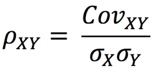
Exposure at Default (EAD)

The exposure at default (EAD) is the predicted expected amount outstanding in case the borrower defaults and essentially is dependent upon the amount to which the bank was exposed to the borrower at the time of default. It changes periodically as the borrower repays his payments to the lender.

Loss given default (LGD)

The loss given default LGD refers to the amount expected to lose by the lender as a proportion of the EAD. Thus, LGD is generally expressed as a percentage.

LGD = (EAD – PV(recovery) – PV(cost))/EAD

With:
PV(recovery) = Present value of recovery discounted till time of default
PV(cost) = Present value of cost of lender discounted till time of default

For instance, a borrower takes a $50,000 auto loan from a bank for purchasing a vehicle. At the time of default, loan has an outstanding balance of $40,000. EAD would thus be $40,000.

Now, the bank takes over the vehicle and sells it for $35,000 for recovery of loan. LGD will be calculated as ($40,000 – $35,000)/$40,000 which is equal to 12.5%. Note that we have assumed the present value of cost here as 0.

Expected Loss

The expected loss is case of default is thus calculated to be PD*EAD*LGD and banks use this methodology in order to better estimate their credit risk and be prepared for any losses to be incurred thus implementing risk management.

Credit Rating

Credit rating describe the creditworthiness of a borrower entity such as a company or a government, which has issued financial debt instruments like loans and bonds. It also applies to individuals who borrow money from their banks to finance the purchase of a scar or residence. It is a means to quantify the credit risk associated with the entity and essentially signifies the likelihood of default.

Credit risk assessment for companies and governments is generally performed by a credit rating agencies which analyses the internal and external, qualitative and quantitative attributes that drive the economic future of the entity. Some examples of such attributes include audited financial statements, annual reports, analyst reports, published news articles, overall industry analysis and future trends, etc.

A credit agency is deemed to provide an independent and impartial opinion of the credit risk and consequent ratings they issue for any entity. Rating agencies S&P Global, Moody’s and Fitch Ratings currently dominate 85% of the global ratings market (as of 2021).

About the author

The article was written in November 2021 by Jayati WALIA (ESSEC Business School, Grande Ecole Program – Master in Management, 2019-2022).

Programming Languages for Quants

October 11, 2021 by Jayati WALIA

Programming Languages for Quants

In this article, Jayati WALIA (ESSEC Business School, Grande Ecole Program – Master in Management, 2019-2022) presents an overview of popular programming languages used in quantitative finance.

Introduction

Finance as an industry has always been very responsive to new technologies. The past decades have witnessed the inclusion of innovative technologies, platforms, mathematical models and sophisticated algorithms solve to finance problems. With tremendous data and money involved and low risk-tolerance, finance is becoming more and more technological and data science, blockchain and artificial intelligence are taking over major decision-making strategies by the power of high processing computer algorithms that enable us to analyze enormous data and run model simulations within nanoseconds with high precision.

This is exactly why programming is a skill which is increasingly in demand. Programming is needed to analyze financial data, compute financial prices (like options or structured products), estimate financial risk measures (like VaR) and test investment strategies, etc. Now we will see an overview of popular programming languages used in modelling and solving problems in the quantitative finance domain.

Python

Python is general purpose dynamic high level programming language (HLL). It’s effortless readability and straightforward syntax allows not just the concept to be expressed in relatively fewer lines of code but also makes it’s learning curve less steep.

Python possesses some excellent libraries for mathematical applications like statistics and quantitative functions such as numpy, scipy and scikit-learn along with the plethora of accessible open source libraries that add to its overall appeal. It supports multiple programming approaches such as object-oriented, functional, and procedural styles.

Python is most popular for data science, machine learning and AI applications. With data science becoming crucial in the financial services industry, it has consequently created an immense demand for Python, making it a programming language of top choice.

C++

The finance world has been dominated by C++ for valid reasons. C++ is one of the essential programming languages in the fintech industry owing to its execution speed. Developers can leverage C++ when they need to programme with advanced computations with low latency in order to process multiple functions fasters such as in High Frequency Trading (HFT) systems. This language offers code reusability (which is crucial in multiple complex quantitative finance projects) to programmers with a diverse library comprising of various tools to execute.

Java

Java is known for its reliability, security and logical architecture with its object-oriented programming to solve complicated problems in the finance domain. Java is heavily used in the sell-side operations of finance involving projects with complex infrastructures and exceptionally robust security demands to run on native as well as cross-platform tools. This language can help manage enormous sets of real-time data with the impeccable security in bookkeeping activity. Financial institutions, particularly investment banks, use Java and C# extensively for their entire trading architecture, including front-end trading interfaces, live data feeds and at times derivatives’ pricing.

R

R is an open source scripting language mostly used for statistical computing, data analytics and visualization along with scientific research and data science. R the most popular language among mathematical data miners, researchers, and statisticians. R runs and compiles on multiple platforms such as Unix, Windows and MacOS. However, it is not the easiest of languages to learn and uses command line scripting which may be complex to code for some.

Scala

Scala is a widely used programming language in banks with Morgan Stanley, Deutsche Bank, JP Morgan and HSBC are among many. Scala is particularly appropriate for banks’ front office engineering needs requiring functional programming (programs using only pure functions that are functions that always return an immutable result). Scala provides support for both object-oriented and functional programming. It is a powerful language with an elegant syntax.

Haskell and Julia

Haskell is a functional and general-purpose programming language with user-friendly syntax, and a wide collection of real-world libraries for user to develop the quant solving application using this language. The major advantage of Haskell is that it has high performance, is robust and is useful for modelling mathematical problems and programming language research.

Julia, on the other hand, is a dynamic language for technical computing. It is suitable for numerical computing, dynamic modelling, algorithmic trading, and risk analysis. It has a sophisticated compiler, numerical accuracy with precision along with a functional mathematical library. It also has a multiple dispatch functionality which can help define function behavior across various argument combinations. Julia communities also provide a powerful browser-based graphical notebook interface to code.

Useful Resources

Websites

QuantInsti Python for Trading

Bankers by Day Programming languages in FinTech

Julia Computing Julia for Finance

R Examples R Basics

About the author

The article was written in October 2021 by Jayati WALIA (ESSEC Business School, Grande Ecole Program – Master in Management, 2019-2022).

Capital Asset Pricing Model (CAPM)

September 6, 2021 by Jayati WALIA

Capital Asset Pricing Model (CAPM)

In this article, Jayati WALIA (ESSEC Business School, Grande Ecole Program – Master in Management, 2019-2022) presents the Capital Asset Pricing Model (CAPM).

Introduction

The Capital Asset Pricing Model (CAPM) is a widely used metrics for the financial analysis of the performance of stocks. It shows the relationship between the expected return and the systematic risk of investing in an asset. The idea behind the model is that the higher the risk in an investment in securities, the higher the returns an investor should expect on his/her investments.

The Capital Asset Pricing Model was developed by financial economists William Sharpe, John Lintner, Jack Treynor and Jan Mossin independently in the 1960s. The CAPM is essentially built on the concepts of the Modern Portfolio Theory (MPT), especially the mean-variance analysis model by Harry Markowitz (1952).

CAPM is very often used in the finance industry to calculate the cost of equity or expected returns from a security which is essentially the discount rate. It is an important tool to compute the Weighted Average Cost of Capital (WACC). The discount rate is then used to ascertain the Present Value (PV) and Net Present Value (NPV) of any business or financial investment.

CAPM formula

The main result of the CAPM is a simple mathematical formula that links the expected return of an asset to its risk measured by the beta of the asset:

CAPM risk beta relation

Where:

E(r_i) represents the expected return of asset i
r_f the risk-free rate
β_i the measure of the risk of asset i
E(r_m) the expected return of the market
E(r_m)- r_f the market risk premium.

The risk premium for asset i is equal to β_i(E(r_m)- r_f), that is the beta of asset i, β_i, multiplied by the risk premium for the market, E(r_m)- r_f.

The formula shows that investors demand a return higher than the risk-free rate for taking higher risk. The equity risk premium is the component that reflects the excess return investors require on their investment.

Let us discuss the components of the Capital Asset Pricing Model individually:

Expected return of the asset: E(r_i)

The expected return of the asset is essentially the minimum return that the investor should demand when investing his/her money in the asset. It can also be considered as the discount rate the investor can utilize to ascertain the value of the asset.

Risk-free interest rate: r_f

The risk-free interest rate is usually taken as the yield on debt issued by the government (the 3-month Treasury bills and the 10-year Treasury bonds in the US) as they are the safest investments. As government bonds have very rare chances of default, their interest rates are considered risk-free.

Beta: β

The beta is a measure of the systematic or the non-diversifiable risk of an asset. This essentially means the sensitivity of an asset price compared to the overall market. The market beta is equal to 1. A beta greater than 1 for an asset signifies that the asset is riskier compared to the overall market, and a beta of less than 1 signifies that the asset is less risky compared to the overall market.

The beta is calculated by using the equation:

CAPM beta formula

Where:

Cov(r_i, r_m) represents the covariance of the return of asset i with the return of the market
σ²(r_m) the variance of the return of the market.

The beta of an asset is defined as the ratio of the covariance between the asset return and the market return, and the variance of the market return.

The covariance is a measure of correlation between two random variables. In practice, the covariance is calculated using historical data for the asset return and the market return.

The variance is a measure of the dispersion of returns. The standard deviation, equal to the square root of the variance, is a measure of the volatility in the market returns over time.

Expected market return

The expected market return is usually computed using historical data of the market. The market is usually represented by a stock index to which the stock belongs to.

For example, for calculating the expected return on APPLE stock, we usually consider the S&P 500 index. Historically, the expected return for the S&P 500 index is around 9%.

Assumptions in Capital Asset Pricing Model

The CAPM considers the following assumptions which forms the basis for the model:

Investors are risk averse and rational – In the CAPM, all investors are assumed to be risk averse. They diversify their portfolio which neutralizes the non-systematic or the diversifiable risk. So, in the end only the systematic or the market risk is considered to calculate the expected returns on the security.
Efficient markets – The markets are assumed to be efficient, thus all investors have equal access to the same information. Also, all the assets are considered to be liquid, and an individual investor cannot influence the future prices of an asset.
No transaction costs – The CAPM assumes that there are no transaction costs, taxes, and restrictions on borrowing or lending activities.
Risk premium – The CAPM model assumes that investors require higher premium for more risk they take (risk aversion).

Example

As an example, lest us consider an investor who wants to calculate the expected return on an investment in APPLE stock. Let’s see how the CAPM can be used in this case.

The risk-free interest rate is taken to be the current yield on 10-year US Treasury bonds. Let us assume that its value is 3%.

The S&P 500 index has an expected return of 9%.

The beta on APPLE stock is 1.25.

The expected return on APPLE stock is equal to 3% + 1.25*(9% – 3%) = 10.50%

Useful resources

Acadedmic articles

Lintner, J. (1965) The Valuation of Risk Assets and the Selection of Risky Investments in Stock Portfolios and Capital Budgets The Review of Economics and Statistics 47(1) 13-37.

Markowitz, H. (1952) Portfolio Selection The Journal of Finance 7(1) 77-91.

Mossin, J. (1966) Equilibrium in a Capital Asset Market Econometrica 34(4) 768-783.

Merton, R.C. (1973) An Intertemporal Capital Asset Pricing Model Econometrica 41(5) 867-887.

Sharpe, W.F. (1964) Capital Asset Prices: A Theory of Market Equilibrium Under Conditions of Risk The Journal of Finance 19(3) 425-442.

Business sources

Mullins, D.W. Jr (1982) Does the Capital Asset Pricing Model Work? Harvard Business Review.

About the author

The article was written in September 2021 by Jayati WALIA (ESSEC Business School, Grande Ecole Program – Master in Management, 2019-2022).

Quantitative risk management

September 6, 2021 by Jayati WALIA

Quantitative risk management

In this article, Jayati WALIA (ESSEC Business School, Grande Ecole Program – Master in Management, 2019-2022) presents Quantitative risk management.

Introduction

Risk refers to the degree of uncertainty in the future value of an investment or the potential losses that may occur. Risk management forms an integral part of any financial institution to safeguard the investments against different risks. The key question that forms the backbone for any risk management strategy is the degree of variability in the profit and loss statement for any investment.

The process of the risk management has three major phases. The first phase is risk identification which mainly focuses on identifying the risk factors to which the institution is exposed. This is followed by risk measurement that can be based on different types of metrics, from monitoring of open positions to using statistical models and Value-at-Risk. Finally, in the third phase risk management is performed by setting risk limits based on the determined risk appetite, back testing (testing the quality of the models on the historical data) and stress testing (assessing the impact of severe but still plausible adverse scenarios).

Different types of risks

There are several types of risks inherent in any investment. They can be categorized in the following ways:

Market risk

An institution can invest in a broad list of financial products including stocks, bonds, currencies, commodities, derivatives, and interest rate swaps. Market risk essentially refers to the risk arising from the fluctuation in the market prices of these assets that an institution trades or invests in. The changes in prices of these underlying assets due to market volatility can cause financial losses and hence, to analyze and hedge against this risk, institutions must constantly monitor the performance of the assets. After measuring the risk, they must also implement necessary measures to mitigate these risks to protect the institution’s capital. Several types of market risks include interest rate risk, equity risk, currency risk, credit spread risk etc.

Credit risk

The risk of not receiving promised repayments due to the counterparty failing to meet its obligations is essentially credit risk. The counterparty risk can arise from changes in the credit rating of the issuer or the client or a default on a due obligation. The default risk can arise from non-payments on any loans offered to the institution’s clients or partners. After the financial crisis of 2008-09, the importance of measuring and mitigating credit risks has increased many folds since the crisis was mainly caused by defaults on payments on sub-prime mortgages.

Operational risk

The risk of financial losses resulting from failed or faulty internal processes, people (human error or fraud) or system, or from external events like fraud, natural calamities, terrorism etc. refers to operational risk. Operational risks are generally difficult to measure and may cause potentially high impacts that cannot be anticipated.

Liquidity risk

The liquidity risk comprises to 2 types namely, market liquidity risk and funding liquidity risk. In market liquidity risk can arise from lack of marketability of an underlying asset i.e., the assets are comparatively illiquid or difficult to sell given a low market demand. Funding liquidity risk on the other hand refers to the ease with which institutions can raise funding and thus institutions must ensure that they can raise and retain debt capital to meet the margin or collateral calls on their leveraged positions.

Strategic risk

Strategic risks can arise from a poor strategic business decisions and include legal risk, reputational risk and systematic and model risks.

Basel Committee on Banking Supervision

The Basel Committee on Banking Supervision (BCBS) was formed in 1974 by central bankers from the G10 countries. The committee is headquartered in the office of the Bank for International Settlements (BIS) in Basel, Switzerland. BCBS is the primary global standard setter for the prudential regulation of banks and provides a forum for regular cooperation on banking supervisory matters. Its 45 members comprise central banks and bank supervisors from 28 jurisdictions. Member countries include Australia, Belgium, Canada, Brazil, China, France, Hong Kong, Italy, Germany, India, Korea, the United States, the United Kingdom, Luxembourg, Japan, Russia, Switzerland, Netherlands, Singapore, South Africa among many others.

Over the years, BCBS has developed influential policy recommendations concerning international banking and financial regulations in order to exercise judicious corporate governance and risk management (especially market, credit and operational risks), known as the Basel Accords. The key function of Basel accords is to manage banks’ capital requirements and ensure they hold enough cash reserves to meet their respective financial obligations and henceforth survive in any financial and/or economic distress.

Over the years, the following versions of the Basel accords have been released in order to enhance international banking regulatory frameworks and improve the sector’s ability to manage with financial distress, improve risk management and promote transparency:

Basel I

The first of the Basel accords, Basel I (also known as Basel Capital Accord) was developed in 1988 and implemented in the G10 countries by 1992. The regulations intended to improve the stability of the financial institutions by setting minimum capital reserve requirements for international banks and provided a framework for managing of credit risk through the risk-weighting of different assets which was also used for assessing banks’ credit worthiness.
However, there were many limitations to this accord, one of which being that Basel I only focused on credit risk ignoring other risk types like market risk, operational risk, strategic risk, macroeconomic conditions etc. that were not covered by the regulations. Also, the requirements posed by the accord were nearly the same for all banks, no matter what the bank’s risk level and activity type.

Basel II

Basel II regulations were developed in 2004 as an extension of Basel I, with a more comprehensive risk management framework and thereby including standardized measures for managing credit, operational and market risks. Basel II strengthened corporate supervisory mechanisms and market transparency by developing disclosure requirements for international regulations inducing market discipline.

Basel III

After the 2008 Financial Crisis, it was perceived by the BCBS that the Basel regulations still needed to be strengthened in areas like more efficient coverage of banks’ risk exposures and quality and measure of the regulatory capital corresponding to banks’ risks.
Basel III intends to correct the miscalculations of risk that were believed to have contributed to the crisis by requiring banks to hold higher percentages of their assets in more liquid instruments and get funding through more equity than debt. Basel III thus tries to strengthen resilience and reduce the risk of system-wide financial shocks and prevent future economic credit events. The Basel III regulations were introduced in 2009 and the implementation deadline was initially set for 2015 however, due to conflicting negotiations it has been repeatedly postponed and currently set to January 1, 2022.

Risk Measures

Efficient risk measurement based on relevant risk measures is a fundamental pillar of the risk management. The following are common measures used by institutions to facilitate quantitative risk management:

Value at risk (VaR)

VaR is the most extensively used risk measure and essentially refers to the maximum loss that should not be exceeded during a specific period of time with a given probability. VaR is mainly used to calculate minimum capital requirements for institutions that are needed to fulfill their financial obligations, decide limits for asset management and allocation, calculate insurance premiums based on risk and set margin for derivatives transactions.
To estimate market risk, we model the statistical distribution of the changes in the market position. Usual models used for the task include normal distribution, the historical distribution and the distributions based on Monte Carlo simulations.

Expected Shortfall

The Expected Shortfall (ES) (also known as Conditional VaR (CVaR), Average Value at risk (AVaR), Expected Tail Loss (ETL) or Beyond the VaR (BVaR)) is a statistic measure used to quantify the market risk of a portfolio. This measure represents the expected loss when it is greater than the value of the VaR calculated with a specific probability level (also known as confidence level).

Credit Risk Measures

Probability of Default (PD) is the probability that a borrower may default on his debt over a period of 1 year. Exposure at Default (EAD) is the expected amount outstanding in case the borrower defaults and Loss given Default (LGD) refers to the amount expected to lose by the lender as a proportion of the EAD. Thus the expected loss in case of default is calculated as PD*EAD*LGD.

Useful resources

Articles

Longin F. (1996) The asymptotic distribution of extreme stock market returns Journal of Business, 63, 383-408.

Longin F. (2000) From VaR to stress testing : the extreme value approach Journal of Banking and Finance, 24, 1097-1130.

Longin F. and B. Solnik (2001) Extreme correlation of international equity markets Journal of Finance, 56, 651-678.

Books

Embrechts P., C. Klüppelberg and T Mikosch (1997) Modelling Extremal Events for Insurance and Finance.

Embrechts P., R. Frey, McNeil A. J. (2022) Quantitative Risk Management, Princeton University Press.

Gumbel, E. J. (1958) Statistics of extremes. New York: Columbia University Press.

Longin F. (2016) Extreme events in finance: a handbook of extreme value theory and its applications Wiley Editions.
Corporate Finance Institute Basel Accords

Other materials

Extreme Events in Finance

QRM Tutorial

About the author

The article was written in September 2021 by Jayati WALIA (ESSEC Business School, Grande Ecole Program – Master in Management, 2019-2022).

Brownian Motion in Finance

January 30, 2024September 6, 2021 by Jayati WALIA

Brownian Motion in Finance

In this article, Jayati WALIA (ESSEC Business School, Grande Ecole Program – Master in Management, 2019-2022) explains the Brownian motion and its applications in finance to model asset prices like stocks traded in financial markets.

Introduction

Stock price movements form a random pattern. The prices fluctuate everyday resulting from market forces like supply and demand, company valuation and earnings, and economic factors like inflation, liquidity, demographics of country and investors, political developments, etc. Market participants try to anticipate stock prices using all these factors and contribute to make price movements random by their trading activities as the financial and economics worlds are constantly changing.

What is a Brownian Motion?

The Brownian motion was first introduced by botanist Robert Brown who observed the random movement of pollen particles due to water molecules under a microscope. It was in the 1900s that the French mathematician Louis Bachelier applied the concept of Brownian motion to asset price behavior for the first time, and this led to Brownian motion becoming one of the most important fundamental of modern quantitative finance. In Bachelier’s theory, price fluctuations observed over a small time period are independent of the current price along with historical behavior of price movements. Combining his assumptions with the Central Limit Theorem, he also deduces that the random behavior of prices can be said to be represented by a normal distribution (Gaussian distribution).

This led to the development of the Random Walk Hypothesis or Random Walk Theory, as it is known today in modern finance. A random walk is a statistical phenomenon wherein stock prices move randomly.

When the time step of a random walk is made infinitesimally small, the random walk becomes a Brownian motion.

Standard Brownian Motion

In context of financial stochastic processes, the Brownian motion is also described as the Wiener Process that is a continuous stochastic process with normally distributed increments. Using the Wiener process notation, an asset price model in continuous time can be expressed as:

brownian motion equation

with dS being the change in asset price in continuous time dt. dX is the random variable from the normal distribution (N(0, 1) or Wiener process). σ is assumed to be constant and represents the price volatility considering the unexpected changes that can result from external effects. μdt together represents the deterministic return within the time interval with μ representing the growth rate of asset price or the ‘drift’.

When the market is modeled with a standard Brownian Motion, the probability distribution function of the future price is a normal distribution.

Geometric Brownian Motion

weiner notation

When the market is modeled with a geometric Brownian Motion, the probability distribution function of the future price is a log-normal distribution.

Properties of a Brownian Motion

Continuity: Brownian motion is the continuous time-limit of the discrete time random walk. It thus, has no discontinuities and is non-differential everywhere.
Finite: The time increments are scaled with the square root of the times steps such that the Brownian motion is finite and non-zero always.
Normality: Brownian motion is normally distributed with zero mean and non-zero standard deviation.
Martingale and Markov Property: Martingale property states that the conditional expectation of the future value of a stochastic process depends on the current value, given information about previous events. The Markov property instead focusses on the ‘no memory’ theory that the expected future value of a stochastic process does not depend on any past values except the current value. Brownian motion follows both these properties.

Simulating Random Walks for Stock Prices

In quantitative finance, a random walk can be simulated programmatically through coding languages. This is essential because these simulations can be used to represent potential future prices of assets and securities and work out problems like derivatives pricing and portfolio risk evaluation.

A very popular mathematical technique of doing this is through the Monte Carlo simulations. In option pricing, the Monte Carlo simulation method is used to generate multiple random walks depicting the price movements of the underlying, each with an associated simulated payoff for the option. These payoffs are discounted back to the present value and the average of these discounted values is set as the option price. Similarly, it can be used for pricing other derivatives, but the Monte Carlo simulation method is more commonly used in portfolio and risk management.

For instance, consider Microsoft stock that has a current price of $258.65 with a growth trend of 55.2% and a volatility of 35.92%.

A plot of daily returns represented as a random normal distribution is:

Normal Distribution

The above figure represents the simulated price path according to the Geometric Brownian motion for the Microsoft stock price. Similarly, a plot of 10 such simulations would be like this:

Microsoft GBM Simulations

Thus, we can see that with just 10 simulations, the prices range from $100 to over $600. We can increase the number of simulations to expand the data set for analysis and use the results for derivatives pricing and many other financial applications.

Brownian motion and the efficient market hypothesis

If the market is efficient in the weak sense (as introduced by Fama (1970)), the current price incorporates all information contained in past prices and the best forecast of the future price is the current price. This is the case when the market price is modelled by a Brownian motion.

▶ Jayati WALIA Black-Scholes-Merton option pricing model

▶ Jayati WALIA Plain Vanilla Options

▶ Jayati WALIA Derivatives Market

Useful Resources

Academic articles

Fama E. (1970) Efficient Capital Markets: A Review of Theory and Empirical Work, Journal of Finance, 25, 383-417.

Fama E. (1991) Efficient Capital Markets: II Journal of Finance, 46, 1575-617.

Books

Malkiel B.G. (2020) A Random Walk Down Wall Street: The Time-tested Strategy for Successful Investing, WW Norton & Co.

Code

Python code for graphs and simulations

Brownian Motion

What is the random walk theory?

About the author

The article was written in August 2021 by Jayati WALIA (ESSEC Business School, Grande Ecole Program – Master in Management, 2019-2022).

Overview

Types of currency overlay strategies

Active currency overlay

Passive currency overlay

Implementing currency overlays

Base currency and benchmark

Hedge ratio

Cost of overlay

Related posts on the SimTrade blog

Useful resources

Academic articles

Business material

About the author

My experience as a credit analyst at Amundi Asset Management

About Amundi

My apprenticeship

Missions

Required skills and knowledge

Three key financial concepts

Credit ratings

Credit spreads

Duration and convexity

Related posts on the SimTrade blog

Useful resources

About the author

Moving averages

What is a moving average?

Types of moving averages

Simple moving average

Exponential-weighted moving average

How to set alpha for an exponential-weighted moving average?

Crossovers

Related posts on the SimTrade blog

Useful resources

About the author

Introduction

Computation methods for implied volatility

Example

Volatility smile

Volatility surface

CBOE Volatility Index

Related posts on the SimTrade blog

Useful resources

Academic articles

Business

About the author

Introduction

Computation of returns

Arithmetic (percentage) returns

Logarithmic returns

Link between arithmetic and logarithmic returns

Components of total returns

Price changes and returns

Internal rate of return (IRR)

Ex ante and ex post returns

Related posts on the SimTrade blog

About the author

Introduction

Calculating VaR using Monte Carlo simulations

Advantages and limitations of Monte Carlo method for VaR

Related posts on the SimTrade blog

Useful resources

About the author

Introduction

How Monte Carlo simulation works

Example: Apple stock

Applications in finance

Related posts on the SimTrade blog

Useful resources

About the author

Assumptions of the BSM Model

The BSM equation

The BSM formulae

Some Criticisms and Limitations

American options

Stocks paying dividends

Constant volatility

Related posts on the SimTrade blog

Useful resources

About the author