Systematic risk and specific risk

November 30, 2021 by Youssef LOURAOUI

In this article, Youssef LOURAOUI (Bayes Business School, MSc. Energy, Trade & Finance, 2021-2022) presents the systematic risk and specific risk of financial assets, two fundamental concepts in asset pricing models and investment management theories more generally.

This article is structured as follows: we introduce the concept of systematic and specific risk. We then explain the mathematical foundation of this concept. We finish with an insight that sheds light on the relationship between diversification and risk reduction.

Portfolio Theory and Risk

Markowitz (1952) and Sharpe (1964) developed a framework on risk based on their significant work in portfolio theory and capital market theory. All rational profit-maximizing investors seek to possess a diversified portfolio of risky assets, and they borrow or lend to get to a risk level that is compatible with their risk preferences under a set of assumptions. They demonstrated that the key risk measure for an individual asset is its covariance with the market portfolio under these circumstances (the beta).

The fraction of an individual asset’s total variance attributable to the variability of the total market portfolio is referred to as systematic risk, which is assessed by the asset’s covariance with the market portfolio. In the article systematic risk, we develop the economic sources of systematic risk: interest rate risk, inflation risk, exchange rate risk, geopolitical risk, and natural risk.

Additionally, due to the asset’s unique characteristics, an individual asset exhibits variance that is unrelated to the market portfolio (the asset’s non-market variance). Specific risk is the term for non-market variance, and it is often seen as minor because it can be eliminated in a large diversified portfolio. In the article specific risk, we develop the economic sources of specific risk: business risk and financial risk.

Mathematical foundations

Following the Capital Asset Pricing Model (CAPM), the return on asset i, denoted by R_i can be decomposed as

img_SimTrade_return_decomposition

Where:

R_i the return of asset i
E(R_i) the expected return of asset i
β_i the measure of the risk of asset i
R_M the return of the market
E(R_M) the expected return of the market
R_M – E(R_M) the market factor
ε_i the specific part of the return of asset i

The three components of the decomposition are the expected return, the market factor and an idiosyncratic component related to asset only. As the expected return is known over the period, there are only two sources of risk: systematic risk (related to the market factor) and specific risk (related to the idiosyncratic component).

The beta of the asset with the market is computed as:

Beta

Where:

σ_i,m : the covariance of the asset return with the market return
σ_m² : the variance of market return

Total risk can be deconstructed into two main blocks:

Total risk formula

The total risk of the asset measured by the variance of asset returns can be computed as:

Decomposition of total risk

Where:

β_i² * σ_m² = systematic risk
σ_εi² = specific risk

In this decomposition of the total variance, the first component corresponds to the systematic risk and the second component to the specific risk.

Effect of diversification on portfolio risk

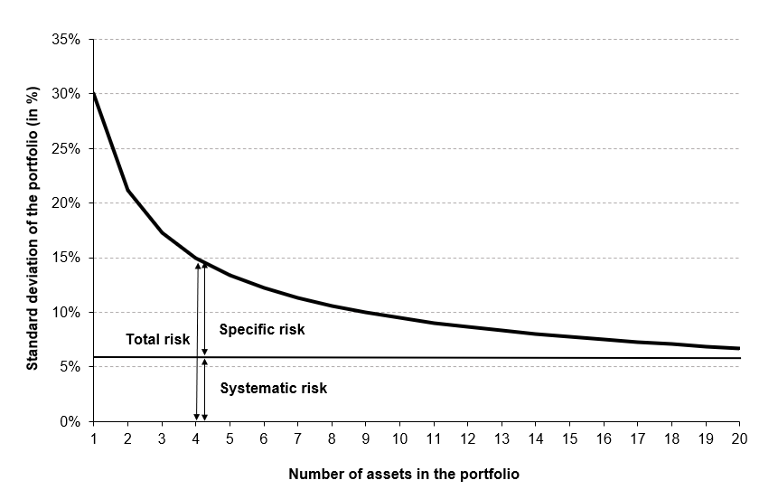
Diversification’s objective is to reduce the portfolio’s standard deviation. This assumes an imperfect correlation between securities. Ideally, as investors add securities, the portfolio’s average covariance decreases. How many securities must be included to create a portfolio that is completely diversified? To determine the answer, investors must observe what happens as the portfolio’s sample size increases by adding securities with some positive correlation. Figure 1 illustrates the effect of diversification on portfolio risk, more precisely on total risk and its two components (systematic risk and specific risk).

Figure 1. Effect of diversification on portfolio risk

Source: Computations from the author.

The critical point is that by adding stocks that are not perfectly correlated with those already held, investors can reduce the portfolio’s overall standard deviation, which will eventually equal that of the market portfolio. At that point, investors eliminated all specific risk but retained market or systematic risk. There is no way to completely eliminate the volatility and uncertainty associated with macroeconomic factors that affect all risky assets. Additionally, investors can reduce systematic risk by diversifying globally rather than just within the United States, as some systematic risk factors in the United States market (for example, US monetary policy) are not perfectly correlated with systematic risk variables in other countries such as Germany and Japan. As a result, global diversification eventually reduces risk to a global systematic risk level.

You can download below two Excel files which illustrate the effect of diversification on portfolio risk.

The first Excel file deals with the case of independent assets with the same profile (risk and expected return).

Figure 2 depicts the risk reduction of total risk in as we increase the number of assets in the portfolio. We manage to reduce half of the overall portfolio volatility by adding five assets to the portfolio. However, the decrease becomes more and more marginal as we add more assets.

Figure 2. Risk reduction of the portfolio. img_SimTrade_systematic_specific_risk_1 Source: Computations from the author.

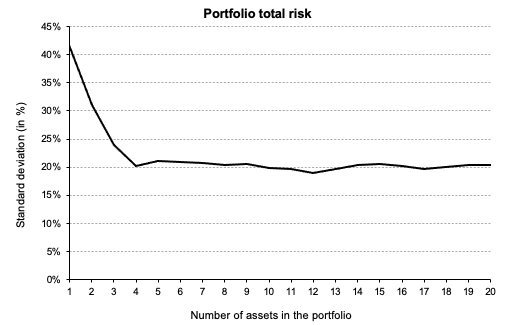
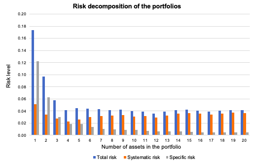
Figure 3 depicts the overall risk reduction of a portfolio. The benefit of diversification are more evident when we add the first 5 assets in the portfolio. As depicted in Figure 2, the diversification starts to fade at a certain point as we keep adding more assets in the portfolio. It can be seen in this figure how the specific risk is considerably reduced as we add more assets because of the effect of diversification. Systematic risk (market risk) is more constant and doesn’t change drastically as we diversify the portfolio. Overall, we can clearly see that diversification helps decrease the total risk of a portfolio considerably.

Figure 3. Risk decomposition of the portfolio. img_SimTrade_systematic_specific_risk_2 Source: Computations from the author.

The second Excel file deals with the case of dependent assets with the different characteristics (expected return, volatility, and market beta).

Academic research

A series of studies examined the average standard deviation for a variety of portfolios of randomly chosen stocks with varying sample sizes. Evans and Archer (1968) and Tole (1982) calculated the standard deviation for portfolios up to a maximum of twenty stocks. The results indicated that the majority of the benefits of diversification were obtained relatively quickly, with approximately 90% of the maximum benefit of diversification being obtained from portfolios of 12 to 18 stocks. Figure 1 illustrates this effect graphically.

This finding has been modified in two subsequent studies. Statman (1987) examined the trade-off between diversification benefits and the additional transaction costs associated with portfolio expansion. He concluded that a portfolio that is sufficiently diversified should contain at least 30–40 stocks. Campbell, Lettau, Malkiel, and Xu (2001) demonstrated that as the idiosyncratic component of an individual stock’s total risk (specific risk) has increased in recent years, it now requires a portfolio to contain more stocks to achieve the same level of diversification. For example, they demonstrated that the level of diversification possible in the 1960s with only 20 stocks would require approximately 50 stocks by the late 1990s (Reilly and Brown, 2012).

Figure 4. Effect of diversification on portfolio risk Source: Computation from the author.

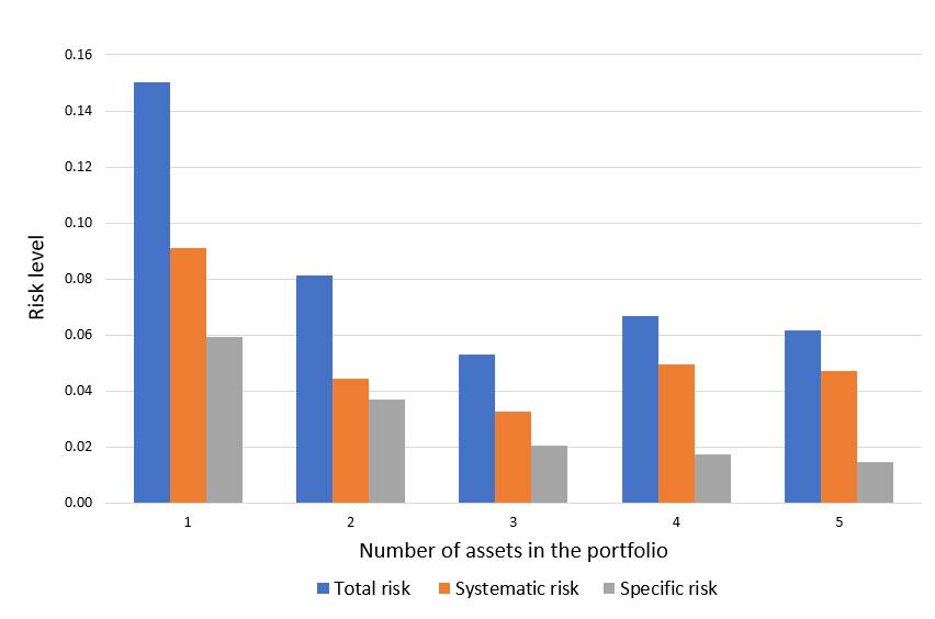
You can download below the Excel file which illustrates the effect of diversification on portfolio risk with real assets (Apple, Microsoft, Amazon, etc.). The effect of diversification on the total risk of the portfolio is already significant with the addition of few stocks.

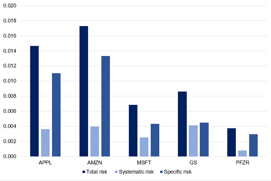
We can appreciate the decomposition of total risk in the below figure with real asset. We can appreciate how asset with low beta had the lowest systematic out of the sample analyzed (i.e. Pfizer). For the whole sample, specific risk is a major concern which makes the major component of risk of each stock. This can be mitigated by holding a well-diversified portfolio that can mitigate this component of risk. Figure 5 depicts the decomposition of total risk for assets (Apple, Microsoft, Amazon, Goldman Sachs and Pfizer).

Figure 5. Decomposition of total risk Source: Computation from the author.

You can download below the Excel file which deconstructs the risk of assets (Apple, Microsoft, Amazon, Goldman Sachs, and Pfizer).

Why should I be interested in this post?

If you’re an investor, understanding the source of risk is essential in order to build balanced portfolios that can withstand market corrections and downturns.

If you are a business school or university undergraduate or graduate student, this content will help you in broadening your knowledge of finance.

Useful resources

Academic research

Campbell, J.Y., Lettau, M., Malkiel, B.G. and Xu, Y. 2001. Have Individual Stocks Become More Volatile? An Empirical Exploration of Idiosyncratic Risk. The Journal of Finance, 56: 1-43.

Evans, J.L., Archer, S.H. 1968. Diversification and the Reduction of Dispersion: An Empirical Analysis. The Journal of Finance, 23(5): 761–767.

Markowitz, H. 1952. Portfolio Selection. The Journal of Finance, 7(1): 77-91.

Mossin, J. 1966. Equilibrium in a Capital Asset Market. Econometrica, 34(4): 768-783.

Reilly, R.K., Brown C.K. 2012. Investment Analysis & Portfolio Management, Tenth Edition. 239-245.

Sharpe, W.F. 1963. A Simplified Model for Portfolio Analysis. Management Science, 9(2): 277-293.

Sharpe, W.F. 1964. Capital Asset Prices: A Theory of Market Equilibrium under Conditions of Risk. The Journal of Finance, 19(3): 425-442.

Statman, M. 1987. How Many Stocks Make a Diversified Portfolio?. The Journal of Financial and Quantitative Analysis, 22(3), 353–363.

Tole T.M. 1982. You can’t diversify without diversifying. The Journal of Portfolio Management. Jan 1982, 8 (2) 5-11.

About the author

The article was written in November 2021 by Youssef LOURAOUI (Bayes Business School, MSc. Energy, Trade & Finance, 2021-2022).

Portfolio

November 26, 2021 by Youssef LOURAOUI

In this article, Youssef LOURAOUI (Bayes Business School, MSc. Energy, Trade & Finance, 2021-2022) elaborates on the concept of portfolio, which is a basic element in asset management.

This article is structured as follows: we introduce the concept of portfolio. We give the basic modelling to define and characterize a portfolio. We then expose the different types of portfolios that investors can rely on to meet their financial goals.

Introduction

An investment portfolio is a collection of assets that an investor owns. These assets can be individual assets such as bonds and stocks or baskets of assets such as mutual funds or exchange-traded funds (ETFs). In a nutshell, this refers to any asset that has the potential to increase in value or generate income. When building a portfolio, investors usually consider the expected return and risk. A well-balanced portfolio includes a variety of investments.

Modelling of portfolios

Portfolio weights

At a point of time, a portfolio is fully defined by the weights (w) of the assets of the universe considered (N assets).

Portfolio weights

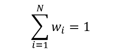
The sum of the portfolio weights adds up to one (or 100%):

Sum of the portfolio weights

The weight of a given asset i can be positive (for a long position in the asset), equal to zero (for a neutral position in the asset) or negative (for a short position in the asset):

Asset weight for a long position

Asset weight for a neutral position

Asset weight for a short position

Short selling is the process of selling a security without owning it. By definition, a short sell occurs when an investor borrows a stock, sells it, and then buys it later back to repay the lender.

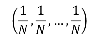
The equally-weighted portfolio is defined as the portfolio with weights that are evenly distributed across the number of assets held:

Equally-weigthed portfolio

Portfolio return: the case of two assets

Over a given period of time, the returns on assets 1 and 2 are equal to r₁ and r₂. In the two-asset portfolio case, the portfolio return r_P is computed as

Return of a 2-asset portfolio

The expected return of the portfolio E(r_P) is computed as

Expected return of a 2-asset portfolio

The standard deviation of the portfolio return, σ(r_P) is computed as

Standard deviation of a 2-asset portfolio return

where:

σ₁ = standard deviation of asset 1
σ₂ = standard deviation of asset 2
σ_1,2 = covariance of assets 1 and 2
ρ_1,2 = correlation of assets 1 and 2

Investing in asset classes with low or no correlation to one another can help you increase portfolio diversification and reduce portfolio volatility. While diversification cannot guarantee a profit or eliminate the risk of investment loss, the ideal scenario is to have a mix of uncorrelated asset classes in order to reduce overall portfolio volatility and generate more consistent long-term returns. Correlation is depicted mathematically as the division of the covariance between the two assets by the individual standard deviation of the asset. Correlation is a more interpretable metric than covariance because it’s measurable within a defined rank. Correlation is measured between -1 and 1, with a high positive correlation showing that the assets move in tandem, while negative correlation depicts securities that have contrary price movements. The holy grail of investing is to invest in securities that offer a low correlation of the portfolio as a whole.

where:

σ_1,2 = covariance of assets 1 and 2
σ₁ = standard deviation of asset 1
σ₂ = standard deviation of asset 2

Correlation is a more interpretable metric than covariance because it’s measurable within a defined rank. Correlation is measured between -1 and 1, with high positive correlation showing that the assets move in tandem, while negative correlation depicts securities that have contrary price movements. The holy grail of investing is to invest in securities that offer a low correlation of the portfolio as a whole.

You can download an Excel file to help you construct a portfolio and compute the expected return and variance of a two-asset portfolio. Just introduce the inputs in the model and the calculations will be performed automatically. You can even draw the efficient frontier to plot the different combinations of portfolios that optimize the risk-return trade-off (to minimize the risk for a given level of expected return or to maximize the expected return for a given level of risk).

Portfolio return: the case of N assets

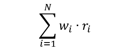
Over a given period of time, the return on asset i is equal to r_i. The portfolio return can be computed as

Portfolio return

The expression of the portfolio return is then used to compute two important portfolio characteristics for investors: the expected performance measured by the average return and the risk measured by the standard deviation of returns.

The expected return of the portfolio is given by

Expected portfolio return

Because relying on multiple assets can get extremely computationally heavy, we can refer to the matrix form for more straightforward use. We basically compute the vector of weight with the vector of returns (NB: we have to pay attention to the dimension and to the properties of matrix algebra).

w = weight vector
r = returns vector

The standard deviation of returns of the portfolio is given by the following equivalent formulas:

Standard deviation of portfolio return

w_i = weight of asset i
w_j = weight of asset j
σ_i = standard deviation of asset i
σ_j = standard deviation of asset j
ρ_i,j = correlation of asset i,j

Standard deviation of portfolio return

where:

w_i² = squared weight of asset I
σ_i² = variance of asset i
w_i = weight of asset i
w_j = weight of asset j
σ_i = standard deviation of asset i
σ_j = standard deviation of asset j
ρ_i,j = correlation of asset i,j

We can use the matrix form for a more straightforward application due to the computational burden associated with relying on multiple assets. Essentially, we multiply the vector of weights with the variance-covariance matrix and the transposed weight vector (NB: we must pay attention to the dimension and to the properties of matrix algebra).

w = weight vector
∑ = variance-covariance matrix
w’ = transpose of weight vector

You can get an Excel file that will help you build a portfolio and calculate the expected return and variance of a three-asset portfolio. Simply enter the data into the model, and the calculations will be carried out automatically. You can even use the efficient frontier to plot the various portfolio combinations that best balance risk and reward (to minimize the risk for a given level of expected return or to maximize the expected return for a given level of risk).

Basic principles on portfolio construction

Diversify

Diversification, a core principle of Markowitz’s portfolio selection theory, is a risk-reduction strategy that entails allocating assets among a variety of financial instruments, sectors, and other asset classes (Markowitz, 1952). In more straightforward terms, it refers to the concept “don’t put all your eggs in one basket.” If the basket is dropped, all eggs are shattered; if many baskets are used, the likelihood of all eggs being destroyed is significantly decreased. Diversification may be accomplished by investments in a variety of companies, asset types (e.g., bonds, real estate, etc.), and/or commodities such as gold or oil.

Diversification seeks to enhance returns while minimizing risk by investing in a variety of assets that will react differently to the same event(s). Portfolio diversification methods should include not just diverse stocks inside and outside of the same industry, but also diverse asset classes, such as bonds and commodities. When there is an imperfect connection between assets (lower than one), the diversification effect occurs. It is a critical and successful risk mitigation method since risk mitigation may be accomplished without jeopardizing profits. As a result, any prudent investor who is cautious (or ‘risk averse’) will diversify to a certain extent.

Portfolio Asset Allocation

The term “asset allocation” refers to the proportion of stocks, bonds, and cash in a portfolio. Depending on your investing strategy, you’ll determine the percentage of each asset type in your portfolio to achieve your objectives. As markets fluctuate over time, your asset allocation is likely to go out of balance. For instance, if Tesla’s stock price increases, the percentage of your portfolio allocated to stocks will almost certainly increase as well.

Portfolio Rebalancing

Rebalancing is a term that refers to the act of purchasing and selling assets in order to restore your portfolio’s asset allocation to its original state and avoid disrupting your plan.

Reduce investment costs as much as possible

Commission fees and management costs are significant expenses for investors. This is especially important if you frequently purchase and sell stocks. Consider using a discount brokerage business to make your investment. Clients are charged much lesser fees by these firms. Also, when investing for the long run, it is advisable to avoid making judgments based on short-term market fluctuations. To put it another way, don’t sell your stocks just because they’ve taken a minor downturn in the near term.

Invest on a regular basis

It is critical to invest on a regular basis in order to strengthen your portfolio. This will not only build wealth over time, but it will also develop the habit of investing discipline.

Buying in the future

It’s possible that you have no idea how a new stock will perform when you buy it. To be on the safe side, avoid putting your entire position to a single investment. Start with a little investment in the stock. If the stock’s performance fulfils your expectations, you can gradually increase your investments until you’ve covered your entire position.

Types of portfolio

We detail below the different types of portfolios usually proposed by financial institutions that investors can rely on to meet their financial goals.

Aggressive Portfolio

As the name implies, an aggressive portfolio is one of the most frequent types of portfolio that takes a higher risk in the pursuit of higher returns. Stocks in an aggressive portfolio have a high beta, which means they present more price fluctuations compared to the market. It is critical to manage risk carefully in this type of portfolio. Keeping losses to a minimal and taking profits are crucial to success. It is suitable for a high-risk appetite investor.

Defensive Portfolio

A defensive portfolio is one that consists of stocks with a low beta. The stocks in this portfolio are largely immune to market swings. The goal of this type of portfolio is to reduce the risk of losing the principal. Fixed-income securities typically make up a major component of a defensive portfolio. It is suitable for a low-risk appetite investor.

Income Portfolio

Another typical portfolio type is one that focuses on investments that generate income from dividends (for stocks), interests (for bonds) or rents (for real estate). An income portfolio invests in companies that return a portion of their profits to shareholders, generating positive cash flow. It is critical to remember that the performance of stocks in an income portfolio is influenced by the current economic condition.

Speculative Portfolio

Among all portfolio types, a speculative portfolio has the biggest risk. Speculative investments could be made of different assets that possess inherently higher risks. Stocks from technology and health-care companies that are developing a breakthrough product, junk bonds, distressed investments among others might potentially be included in a speculative portfolio. When establishing a speculative portfolio, investors must exercise caution due to the high risk involved.

Hybrid Portfolio

A hybrid portfolio is one that includes passive investments and offers a lot of flexibility. The cornerstone of a hybrid portfolio is typically made up of blue-chip stocks and high-grade corporate or government bonds. A hybrid portfolio provides diversity across many asset classes while also providing stability by combining stocks and bonds in a predetermined proportion.

Socially Responsible Portfolio

A socially responsible portfolio is based on environmental, social, and governance (ESG) criteria. It allows investors to make money while also doing good for society. Socially responsible or ESG portfolios can be structured for any level of risk or investment aim and can be built for growth or asset preservation. The important thing is that they prefer stocks and bonds that aim to reduce or eliminate environmental impact or promote diversity and equality.

Why should I be interested in this post?

Portfolio management’s objective is to optimize the returns on the entire portfolio, not just on one or two stocks. By monitoring and maintaining your investment portfolio, you can accumulate a sizable capital to fulfil a variety of financial objectives, including retirement planning. This article helps to understand the grounding fundamentals behind portfolio construction and investing.

Useful resources

Academic research

Mangram, M.E., 2013. A simplified perspective of the Markowitz Portfolio Theory. Global Journal of Business Research, 7(1): 59-70.

Markowitz, H., 1952. Portfolio Selection. The Journal of Finance, 7(1): 77-91.

Business analysis

Edelweiss, 2021.What is a portfolio?

Forbes, 2021.Investing basics: What is a portfolio?

JP Morgan Asset Management, 2021.Glossary of investment terms: Portfolio

About the author

The article was written in November 2021 by Youssef LOURAOUI (Bayes Business School, MSc. Energy, Trade & Finance, 2021-2022).

Black-Litterman Model

November 21, 2021 by Youssef LOURAOUI

In this article, Youssef LOURAOUI (Bayes Business School, MSc. Energy, Trade & Finance, 2021-2022) presents the Black-Litterman model, used to determine optimal asset allocation in a portfolio. The Black-Litterman model takes the Markowitz model one step further: it incorporates an investor’s own views in determining asset allocations.

This article is structured as follows: we introduce the Black-Litterman model. We then present the mathematical foundations of the model to understand how the method is derived. We finish with an example to illustrate how we can implement a Black-Litterman asset allocation in practice.

Introduction

The Black-Litterman asset allocation model, developed by Fischer Black and Robert Litterman in the early 1990’s, is a complex method for dealing with unintuitive, highly concentrated, input-sensitive portfolios produced by the Markowitz model. The most likely reason why more portfolio managers do not employ the Markowitz paradigm, in which return is maximized for a given level of risk, is input sensitivity, which is a well-documented problem with mean-variance optimization.

The Black-Litterman model employs a Bayesian technique to integrate an investor’s subjective views on expected returns for one or more assets with the market equilibrium expected returns (prior distribution) of expected returns to get a new, mixed estimate of expected returns. The new vector of expected returns (the posterior distribution) is a complex, weighted average of the investor’s views and the market equilibrium.

The purpose of the Black-Litterman model is to develop stable, mean-variance efficient portfolios based on an investor’s unique insights that overcome the problem of input sensitivity. According to Lee (2000), the Black-Litterman Model “essentially mitigates” the problem of estimating error maximization (Michaud, 1989) by dispersing errors throughout the vector of expected returns.

The vector of expected returns is the most crucial input in mean-variance optimization; yet, Best and Grauer (1991) demonstrate that this input can be very sensitive in the final result. Black and Litterman (1992) and He and Litterman (1999) investigate various potential projections of expected returns in their search for a fair starting point: historical returns, equal “mean” returns for all assets, and risk-adjusted equal mean returns. They demonstrate that these alternate forecasts result in extreme portfolios, which have significant long and short positions concentrated in a small number of assets.

Mathematical foundation of Black-Litterman model

It is important to introduce the Black-Litterman formula and provide a brief description of each of its elements. In the formula below, the integer k is used to represent the number of views and the integer n to express the number of assets in the investment set (NB: the superscript ’ indicates the transpose and -1 indicates the inverse).

Where:

E[R] = New (posterior) vector of combined expected return (n x 1 column vector)
τ = Scalar
Σ = Covariance matrix of returns (n x n matrix)
P = Identifies the assets involved in the views (k x n matrix or 1 x n row vector in the special case of 1 view)
Ω = Diagonal covariance matrix of error terms in expressed views representing the level of confidence in each view (k x k matrix)
П = Vector of implied equilibrium expected returns (n x 1 column vector)
Q = Vector of views (k x 1 column vector)

Traditionally, personal views are used for prior distribution. Then observed data is used to generate a posterior distribution. The Black-Litterman Model assumes implied returns as the prior distribution and personal views alter it. The basic procedure to find the Black-Litterman model is: 1) Find implied returns 2) Formulate investor views 3) Determine what the expected returns are 4) Find the asset allocation for the optimal portfolio.

Black-Litterman asset allocation in practice

An investment manager’s views for the expected return of some of the assets in a portfolio are frequently different from the the Implied Equilibrium Return Vector (Π), which represents the market-neutral starting point for the Black-Litterman model. representing the uncertainty in each view. Such views can be represented in absolute or relative terms using the Black-Litterman Model. Below are three examples of views stated in the Black and Litterman model (1990).

View 1: Merck (MRK) will generate an absolute return of 10% (Confidence of View = 50%).
View 2: Johnson & Johnson (JNJ) will outperform Procter & Gamble (PG) by 3% (Confidence of View = 65%).
View 3: GE (GE) will beat GM (gm), Wal-Mart (WMT), and Exxon (XOM) by 1.5 percent (Confidence of View = 30%).

An absolute view is exemplified by View 1. It instructs the Black-Litterman model to set Merck’s return at 10%.

Views 2 and 3 are relative views. Relative views are more accurate representations of how investment managers feel about certain assets. According to View 2, Johnson & Johnson’s return will be on average 3 percentage points higher than Procter & Gamble’s. To determine if this will have a good or negative impact on Johnson & Johnson in comparison to Procter & Gamble, their respective Implied Equilibrium returns must be evaluated. In general (and in the absence of constraints and other views), the model will tilt the portfolio towards the outperforming asset if the view exceeds the difference between the two Implied Equilibrium returns, as shown in View 2.

View 3 shows that the number of outperforming assets does not have to equal the number of failing assets, and that the labels “outperforming” and “underperforming” are relative terms. Views that include several assets with a variety of Implied Equilibrium returns are less intuitive, generalizing more challenges. In the absence of constraints and other views, the view’s assets are divided into two mini-portfolios: a long and a short portfolio. The relative weighting of each nominally outperforming asset is proportional to that asset’s market capitalization divided by the sum of the market capitalization of the other nominally outperforming assets of that particular view. Similarly, the relative weighting of each nominally underperforming asset is proportional to that asset’s market capitalization divided by the sum of the market capitalizations of the other nominally underperforming assets. The difference between the net long and net short positions is zero. The real outperforming asset(s) from the expressed view may not be the mini-portfolio that receives the good view. In general, the model will overweight the “outperforming” assets if the view is greater than the weighted average Implied Equilibrium return differential.

Why should I be interested in this post?

Modern Portfolio Theory (MPT) is at the heart of modern finance and its core foundations are structuring the modern investing panorama. MPT has established itself as the foundation for modern financial theory and practice. MPT’s premise is that beating the market is difficult, and those that do it by diversifying their portfolios appropriately and accepting higher-than-average investment risks.

MPT has been around for almost sixty years, and its popularity is unlikely to wane anytime soon. Its theoretical contributions have laid the groundwork for more theoretical research in the field of portfolio theory. Markowitz’s portfolio theory, however, is vulnerable to and dependent on continuing ‘probabilistic’ development and expansion. This article shed light on an enhancement of the initial Markowitz work by going a step further: to incorporate the views of the investors in the asset allocation process.

Useful resources

Academic research

Best, M.J., and Grauer, R.R. 1991. On the Sensitivity of Mean-Variance-Efficient Portfolios to Changes in Asset Means: Some Analytical and Computational Results.The Review of Financial Studies, 315-342.

Black, F. and Litterman, R. 1990. Asset Allocation: Combining Investors Views with Market Equilibrium. Goldman Sachs Fixed Income Research working paper

Black, F. and Litterman, R. 1991. Global Asset Allocation with Equities, Bonds, and Currencies. Goldman Sachs Fixed Income Research working paper

Black, F. and Litterman, R. 1992. Global Portfolio Optimization.Financial Analysts Journal, 28-43.

He, G. and Litterman, R. 1999. The Intuition Behind Black-Litterman Model Portfolios. Goldman Sachs Investment Management Research, working paper.

Idzorek, T.M. 2002. A step-by-step guide to Black-Litterman model. Incorporating user-specified confidence levels. Working Paper, 2-11.

Lee, W., 2000, Advanced theory and methodology of tactical asset allocation. Fabozzi and Associates Publications.

Markowitz, H., 1952. Portfolio Selection. The Journal of Finance, 7(1): 77-91.

Michaud, R.O. 1989. The Markowitz Optimization Enigma: Is Optimized Optimal?. Financial Analysts Journal, 31-42.

Mossin, J. 1966. Equilibrium in a Capital Asset Market. Econometrica, 34(4): 768-783.

Sharpe, W.F. 1963. A Simplified Model for Portfolio Analysis. Management Science, 9(2): 277-293.

Sharpe, W.F. 1964. Capital Asset Prices: A Theory of Market Equilibrium under Conditions of Risk. The Journal of Finance, 19(3): 425-442.

About the author

The article was written in November 2021 by Youssef LOURAOUI > (Bayes Business School, MSc. Energy, Trade & Finance, 2021-2022).

Passive Investing

November 21, 2021 by Youssef LOURAOUI

In this article, Youssef LOURAOUI (Bayes Business School, MSc. Energy, Trade & Finance, 2021-2022) elaborates on the concept of passive investing.

This article will offer a concise summary of the academic literature on passive investment. After that, we’ll discuss the fundamental principles of passive investment. The article will finish by establishing a link between passive strategies and the Efficient Market Hypothesis.

Review of academic literature on passive investing

We can retrace the foundations of passive investing to the theory of portfolio construction developed by Harry Markowitz. For his theoretical implications, Markowitz’s work is widely regarded as a pioneer in financial economics and corporate finance. For his contributions to these disciplines, which he developed in his thesis “Portfolio Selection” published in The Journal of Finance in 1952, Markowitz received the Nobel Prize in economics in 1990. His ground-breaking work set the foundation for what is now known as ‘Modern Portfolio Theory’ (MPT).

William Sharpe (1964), John Lintner (1965), and Jan Mossin (1966) separately developed the Capital Asset Pricing Model (CAPM). The CAPM was a huge evolutionary step forward in capital market equilibrium theory because it enabled investors to appropriately value assets in terms of their risk. The asset management industry intended to capture the market portfolio return in the late 1970s, defined as a hypothetical collection of investments that contains every kind of asset available in the investment universe, with each asset weighted in proportion to its overall market participation. A market portfolio’s expected return is the same as the market’s overall expected return. But as financial research evolved and some substantial contributions were made, new factor characteristics emerged to capture some additional performance.

Core principles of passive investing

Positive outlook: The core element of passive investing is that investors can expect the stock market to rise over the long run. A portfolio that mimics the market will appreciate in lockstep with it.

Low cost: A passive strategy has low transaction costs (commissions and market impact) due to its steady approach and absence of frequent trading. While management fees required by funds are unavoidable, most exchange traded funds (ETFs) – the vehicle of choice for passive investors – charge much below 1%.

Diversification: Passive strategies automatically provide investors with a cost-effective method of diversification. This is because index funds diversify their risk by investing in a diverse range of securities from their target benchmarks.

Reduced risk: Diversification almost usually results in lower risk. Investors can also diversify their holdings more within sectors and asset classes by investing in more specialized index funds.

Passive investing and Efficient Market Hypothesis

The Efficient Market Hypothesis (EMH) asserts that markets are efficient, meaning that all information is incorporated into market prices (Fama, 1970). The passive investing strategy is built on the concept of “buy-and-hold,” or keeping an investment position for a lengthy period without worrying about market timing. This latter technique is frequently implemented through the purchase of exchange-traded funds (ETF) that aim to closely match a given benchmark to produce a performance that is comparable to the underlying index or benchmark. The index might be broad-based, such as the S&P500 index in the US equity market for instance, or more specialized, such as an index that monitors a specific sector or geographical zone.

A study from Bloomberg on index funds suggests that passive investments lead 11.6 trillion $ in the US domestic equity-fund market. Passive investing accounts for approximately 54% of the market, owing largely to the growth of funds tracking the S&P 500, the total US stock market, and other broad US indexes. Large-cap stocks in the United States are widely recognized as the world’s most efficient equity market, contributing to passive investing’s dominance. The $6.2 trillion in passive assets represents less than a sixth of the US stock market, which currently has a market capitalization of approximately $40.4 trillion (Bloomberg, 2021).

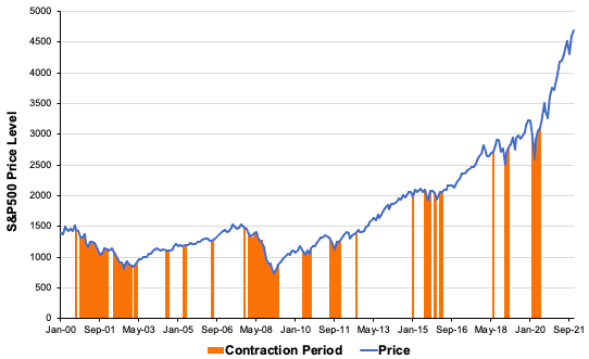
Figure 1 depicts the historical monthly returns of the S&P500 highlighting the contraction periods in orange. It is considered as a key benchmark that is heavily tracked by passive instruments like Exchange Traded Funds and Mutual Funds. In a two-decade timeframe analysis, the S&P managed to offer an annualised 5.56% return on average coupled with a 15.16% volatility.

Figure 1. S&P500 historical returns (Jan 2000 – November 2021).

Source: Computation by the author (data source: Thomson Reuters).

Estimation of the S&P500 return

You can download an Excel file with data for the S&P500 index returns (used as a representation of the market).

Why should I be interested in this post?

If you are a business school or university undergraduate or graduate student, this content will help you in grasping the concept of passive investing, which is in practice key to investors, and which has attracted a lot of attention in academia.

Useful resources

Academic research

Lintner, J. 1965a. The Valuation of Risk Assets and the Selection of Risky Investments in Stock Portfolios and Capital Budgets. The Review of Economics and Statistics, 47(1): 13-37.

Lintner, J. 1965b. Security Prices, Risk and Maximal Gains from Diversification. The Journal of Finance, 20(4): 587-615.

Mangram, M.E., 2013. A simplified perspective of the Markowitz Portfolio Theory. Global Journal of Business Research, 7(1): 59-70.

Markowitz, H., 1952. Portfolio Selection. The Journal of Finance, 7(1): 77-91.

Mossin, J. 1966. Equilibrium in a Capital Asset Market.Econometrica, 34(4): 768-783.

Sharpe, W.F. 1963. A Simplified Model for Portfolio Analysis.Management Science, 9(2): 277-293.

Sharpe, W.F. 1964. Capital Asset Prices: A theory of Market Equilibrium under Conditions of Risk. The Journal of Finance, 19(3): 425-442.

Business analysis

JP Morgan Asset Management, 2021.Glossary of investment terms: Passive Investing

Bloomberg, 2021. Passive likely overtakes active by 2026, earlier if bear market

About the author

The article was written in November 2021 by Youssef LOURAOUI (Bayes Business School, MSc. Energy, Trade & Finance, 2021-2022).

Beta

November 20, 2021 by Youssef LOURAOUI

In this article, Youssef LOURAOUI (Bayes Business School, MSc. Energy, Trade & Finance, 2021-2022) explains the concept of beta, one of the most fundamental concepts in the financial industry, which is heavily used in asset management to assess the risk of assets and portfolios.

This article is structured as follows: we introduce the concept of beta in asset management. Next, we present the mathematical foundations of the concept. We finish with an interpretation of beta values for risk analysis.

Introduction

The (market) beta represents the sensitivity of an individual asset or a portfolio to the fluctuations of the market. This risk measure helps investors to predict the movements of their assets according to the movements of the market overall. It measures the asset risk in comparison with the systematic risk inherent to the market.

In practice, the beta for a portfolio (fund) in respect to the market M represented by a predefined index (the S&P 500 index for example) indicates the fund’s sensitivity to the index. Essentially, the fund’s beta to the index attempts to capture the amount of money made (or lost) when the index increases (or decreases) by a specified amount.

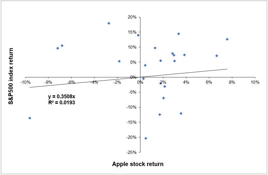
Graphically, the beta represents the slope of the straight line through a regression of data points between the asset return in comparison to the market return for different time periods. It is a traditional risk measure used in the asset management industry. To give a more insightful explanation, a regression analysis has been performed using data for the Apple stock (APPL) and the S&P500 index to see how the stock behaves in relation to the market fluctuations (monthly data for the period July 2018 – June 2020). Figure 1 depicts the regression between Apple stock and the S&P500 index (excess) returns. The estimated beta is between zero and one (beta = 0.3508), which indicates that the stock price fluctuates less than the market index.

Figure 1. Linear regression of the Apple stock return on the S&P500 index return.

Source: Computation by the author (data source: Thomson Reuters).

Mathematical derivation of Beta

Use of beta

William Sharpe, John Lintner, and Jan Mossin separately developed key capital markets theory as a result of Markowitz’s previous works: the Capital Asset Pricing Model (CAPM). The CAPM was a huge evolutionary step forward in capital market equilibrium theory since it enabled investors to appropriately value assets in terms of systematic risk, defined as the market risk which cannot be neutralized by the effect of diversification.

The CAPM expresses the expected return of an asset a function of the risk-free rate, the beta of the asset, and the expected return of the market. The main result of the CAPM is a simple mathematical formula that links the expected return of an asset to these different components. For an asset i, it is given by:

CAPM risk beta relation

Where:

E(r_i) represents the expected return of asset i
r_f the risk-free rate
β_i the measure of the risk of asset i
E(r_m) the expected return of the market
E(r_m)- r_f the market risk premium.

The risk premium for asset i is equal to β_i(E(r_m)- r_f), that is the beta of asset i, β_i, multiplied by the risk premium for the market, E(r_m)- r_f.

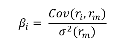
In this model, the beta (β) parameter is a key parameter and is defined as:

CAPM beta formula

Where:

Cov(r_i, r_m) represents the covariance of the return of asset i with the return of the market
σ²(r_m) the variance of the return of the market.

Excel file to compute the beta

You can download below an Excel file with data for Apple stock returns and the S&P500 index returns (used as a representation of the market). This Excel file computes the beta of apple with the S&P500 index.

Interpretation of the beta

Beta helps investors to explain how the asset moves compared to the market. More specifically, we can consider the following cases for beta values:

β = 1 indicates a fluctuation between the asset and its benchmark, thus the asset tends to move at a similar rate than the market fluctuations. A passive ETF replicating an index will present a beta close to 1 with its associated index.
0 < β < 1 indicates that the asset moves at a slower rate than market fluctuations. Defensive stocks, stocks that deliver consistent returns without regarding the market state like P&G or Coca Cola in the US, tend to have a beta with the market lower than 1.
β > 1 indicates a more aggressive effect of amplification between the asset price movements with the market movements. Call options tend to have higher betas than their underlying asset.
β = 0 indicates that the asset or portfolio is uncorrelated to the market. Govies, or sovereign debt bonds, tend to have a beta-neutral exposure to the market.
β < 0 indicates an inverse effect of market fluctuation impact in the asset volatility. In this sense, the asset would behave inversely in terms of volatility compared to the market movements. Put options and Gold typically tend to have negative betas.

Why should I be interested in this post?

If you are a business school or university student, this post will help you to understand the fundamentals of investment.

Useful resources

Academic research

Fama, Eugene F. 1965. The Behavior of Stock Market Prices.Journal of Business 37: January 1965, 34-105.

Fama, Eugene F. 1967. Risk, Return, and General Equilibrium in a Stable Paretian Market. Chicago, IL: University of Chicago.Unpublished manuscript.

Fama, Eugene F. 1968. Risk, Return, and Equilibrium: Some Clarifying Comments. Journal of Finance, (23), 29-40.

Lintner, J. 1965a. The Valuation of Risk Assets and the Selection of Risky Investments in Stock Portfolios and Capital Budgets. The Review of Economics and Statistics 47(1): 13-37.

Lintner, J. 1965b. Security Prices, Risk and Maximal Gains from Diversification. The Journal of Finance 20(4): 587-615.

Mangram, M.E., 2013. A simplified perspective of the Markowitz Portfolio Theory. Global Journal of Business Research, 7(1): 59-70.

Markowitz, H., 1952. Portfolio Selection. The Journal of Finance, 7(1): 77-91.

Mossin, J. 1966. Equilibrium in a Capital Asset Market. Econometrica 34(4): 768-783.

Sharpe, W.F. 1963. A Simplified Model for Portfolio Analysis. Management Science 9(2): 277-293.

Sharpe, W.F. 1964. Capital Asset Prices: A Theory of Market Equilibrium under Conditions of Risk. The Journal of Finance 19(3): 425-442.

Business analysis

JP Morgan Asset Management, 2021. Glossary of investment terms: Beta

Man Institute, 2021. How to calculate the Beta of a portfolio to a factor

Nasdaq, 2021. Beta

About the author

The article was written in November 2021 by Youssef LOURAOUI (Bayes Business School, MSc. Energy, Trade & Finance, 2021-2022).

Alpha

November 20, 2021 by Youssef LOURAOUI

In this article, Youssef LOURAOUI (Bayes Business School, MSc. Energy, Trade & Finance, 2021-2022) elaborates on the concept of alpha, one of the fundamental parameters for portfolio performance measure.

This article is structured as follows: we introduce the concept of alpha in asset management. Next, we present some interesting academic findings on the alpha. We finish by presenting the mathematical foundations of the concept.

Introduction

The alpha (also called Jensen’s alpha) is defined as the additional return delivered by the fund manager on the overall performance of the portfolio compared to the market performance (Jensen, 1968). A key issue in finance (and particularly in portfolio management) has been evaluating the performance of portfolio managers. The term ‘performance’ encompasses at least two independent dimensions (Sharpe, 1967): 1) The portfolio manager’s ability to boost portfolio returns by successful forecasting of future security prices; and 2) The portfolio manager’s ability to minimize (via “efficient” diversification) the amount of “insurable risk” borne by portfolio holders.

The primary hurdle to evaluating a portfolio’s performance in these two categories has been a lack of a solid grasp of the nature and assessment of “risk”. Risk aversion appears to predominate in the capital markets, and as long as investors accurately perceive the “riskiness” of various assets, this indicates that “risky” assets must on average give higher returns than less “risky” assets. Thus, when evaluating portfolios’ performance, the implications of varying degrees of risk on their returns must be considered (Sharpe, 1967).

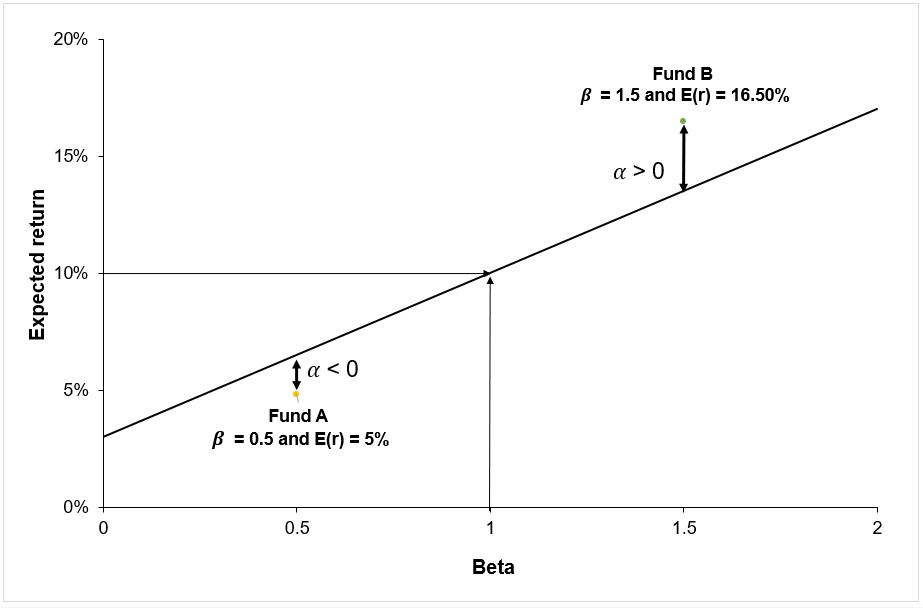
One way of representing the performance is by linking the performance of a portfolio to the security market line (SML). Figure 1 depicts the relation between the portfolio performance in relation to the security market line. As illustrated in Figure 1 below, Fund A has a negative alpha as it is located under the SML, implying a negative performance of the fund manager compared to the market. Fund B has a positive alpha as it is located above the SML, implying a positive performance of the fund manager compared to the market.

Figure 1. Alpha and the Security Market Line

Source: Computation by the author.

You can download below an Excel file with data to compute Jensen’s alpha for fund performance analysis.

Academic Literature

Jensen develops a risk-adjusted measure of portfolio performance that quantifies the contribution of a manager’s forecasting ability to the fund’s returns. In the first empirical study to assess the outperformance of fund managers, Jensen aimed at quantifying the predictive ability of 115 mutual fund managers from 1945 to 1964. He looked at their ability to produce returns above the expected return given the risk level of each portfolio. Not only does the evidence on mutual fund performance indicate that these 115 funds on average were unable to forecast security prices accurately enough to outperform a buy-and-hold strategy, but there is also very little evidence that any individual fund performed significantly better than what we would expect from mutual random chance. Additionally, it is critical to highlight that these conclusions hold even when fund returns are measured net of management expenses (that is assume their bookkeeping, research, and other expenses except brokerage commissions were obtained free). Thus, on average, the funds did not appear to be profitable enough in their trading activity to cover even their brokerage expenses.

Mathematical derivation of Jensen’s alpha

The portfolio performance metric given below is derived directly from the theoretical results of Sharpe (1964), Lintner (1965a), and Treynor (1965) capital asset pricing models. All three models assume that (1) all investors are risk-averse and single-period expected utility maximizers, (2) all investors have identical decision horizons and homogeneous expectations about investment opportunities, (3) all investors can choose between portfolios solely based on expected returns and variance of returns, (4) all transaction costs and taxes are zero, and (5) all assets are infinitely fungible. With the extra assumption of an equilibrium capital market, each of the three models produces the following equation for the expected one-period return defined by (Jensen, 1968):

E(r): the expected return of the fund
r_f: the risk-free rate
E(r_m): the expected return of the market
β(E(r_m) – r_f): the systematic risk of the portfolio
α: the alpha of the portfolio (Jensen’s alpha)

Why should I be interested in this post?

If you are a business school or university student, this post will help you to understand the fundamentals of investment.

Useful resources

Academic research

Fama, Eugene F. 1965. The Behavior of Stock Market Prices.Journal of Business 37, 34-105.

Fama, Eugene F. 1967. Risk, Return, and General Equilibrium in a Stable Paretian Market. Chicago, IL: University of Chicago.Unpublished manuscript.

Fama, Eugene F. 1968. Risk, Return, and Equilibrium: Some Clarifying Comments. Journal of Finance, 23, 29-40.

Lintner, John. 1965a. Security Prices, Risk, and Maximal Gains from Diversification. Journal of Finance, 20, 587-616.

Lintner, John. 1965b. The Valuation of Risk Assets and the Selection of Risky Investments in Stock Portfolios and Capital Budgets.Review of Economics and Statistics 47, 13-37.

Markowitz, H., 1952. Portfolio Selection. The Journal of Finance, 7, 77-91.

Sharpe, William F. 1963. A Simplified Model for Portfolio Analysis. Management Science, 19, 425-442.

Sharpe, William F. 1964. Capital Asset Prices: A Theory of Market Equilibrium under Conditions of Risk. Journal of Finance, 19, 425-442.

Sharpe, William F. 1966. Mutual Fund Performance. Journal of Business39, Part 2: 119-138.

Treynor, Jack L. 1965. How to Rate Management of Investment Funds.Harvard Business Review 18, 63-75.

Business analysis

JP Morgan Asset Management, 2021.Glossary of investment terms: Alpha

About the author

The article was written in November 2021 by Youssef LOURAOUI (Bayes Business School,, MSc. Energy, Trade & Finance, 2021-2022).

Security Market Line (SML)

November 20, 2021 by Youssef LOURAOUI

In this article, Youssef LOURAOUI (Bayes Business School, MSc. Energy, Trade & Finance, 2021-2022) presents the Security Market Line (SML), a key concept in asset pricing derived from the Capital Asset Pricing Model (CAPM).

This article is structured as follows: we first introduce the concept of Security Market Line (SML). We then present the mathematical foundations of the SML. We finish by presenting an investment strategy that can be implemented relying on the SML.

Security Market Line

The SML reflects the risk-return combinations accessible in the capital market at any given time for all risky assets. Investors would choose investments based on their risk appetites; some would only consider low-risk investments, while others would welcome high-risk investments. The SML is derived from the Capital Asset Pricing Model (CAPM), which describes the trade-off between risk and expected return for efficient portfolios.

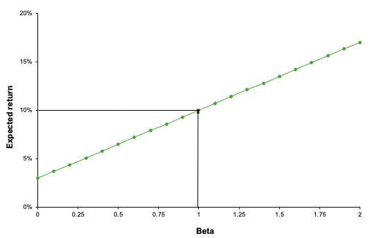
The expected relationship between risk and return is depicted in Figure 1. It demonstrates that as perceived risk increases, investors’ required rates of return increase.

Figure 1. Security Market Line.

Source: Computation by the author.

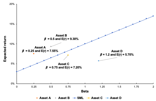
Under the CAPM framework, all investors will choose a position on the capital market line by borrowing or lending at the risk-free rate, since this maximizes the return for a given level of risk. Whereas the CML indicates the rates of return of a specific portfolio, the SML represents the risk and return of the market at a given point in time and indicates the expected returns of individual assets. Also, while the measure of risk in the CML is the standard deviation of returns (total risk), the measure of risk in the SML is the systematic risk, or beta. Figure 2 depicts the SML line combined with four different assets. Asset A and B are above the SML line, which implies that they are overvalued. Asset C and D are below the SML which implies that they are undervalued. From Figure 2, we can implement an investment strategy by going long if the asset or portfolio lies under the SML and going short if the asset or portfolio is greater than the SML.

Figure 2. Security Market Line with a plot of different assets.

Source: Computation by the author.

Mathematical foundation

The SML plots an individual security’s expected rate of return against systematic, undiversifiable risk. The risk associated with an individual risky security is determined by the volatility of the security’s return, not by the market portfolio’s return. Individual risky securities bear a proportional share of the systematic risk. The only risk that an investor should be compensated for is systematic risk, which cannot be neutralized through diversification. This risk is quantified using the beta, which refers to a security’s sensitivity to market fluctuations. The slope of the SML is equal to the market risk premium and reflects the risk-reward trade-off at a particular point in time. We can define the line of the SML as:

Mathematically, we can deconstruct the SML as:

SML_formula

Where

E(R_i) represents the expected return of asset i
R_f is the risk-free interest rate
β_i measures the systematic risk of asset i
E(R_M) represents the expected return of the market
E[R_M – R_f] represents the market risk premium.

Beta and the market factor

William Sharpe (1964), John Lintner (1965), and Jan Mossin (1966) independently developed the Capital Asset Pricing Model (CAPM). The CAPM was a significant evolutionary step forward in capital market equilibrium theory because it allowed investors to value assets correctly in terms of risk. The CAPM makes a distinction between two forms of risk: systematic and specific risk. Systematic risk refers to the risk posed by the market’s basic structure, its participants, and all non-diversifiable elements such as monetary policy, political events, and natural disasters. By contrast, specific risk refers to the risk inherent in a particular asset and so is diversifiable. As a result, the CAPM solely captures systematic risk via the beta measure, with the market’s beta equal to one, lower-risk assets having a beta less than one, and higher-risk assets having a beta larger than one.

In the late 1970s, the portfolio management industry sought to replicate the market portfolio return, but as financial research advanced and significant contributions were made, it enabled the development of additional factor characteristics to capture additional performance. This resulted in the development of what is now known as factor investing.

Estimation of the Security Market Line

You can download an Excel file with data to estimate the Security Market Line.

Why should I be interested in this post?

The security market line is frequently used by portfolio managers and investors to determine the suitability of an investment product for inclusion in a portfolio. The SML is useful for determining whether a security’s expected return is favourable in comparison to its level of risk. The SML is frequently used to compare two similar securities that offer approximately the same rate of return to determine which one has the lowest inherent market risk in relation to the expected rate of return. Additionally, the SML can be used to compare securities of comparable risk to determine which one offers the highest expected return for that level of risk.

If you are a business school or university undergraduate or graduate student, this content will help you in broadening your knowledge of finance.

Useful resources

Academic research

Drake, P. and Fabozzi, F., 2010. The Basics of Finance: An Introduction to Financial Markets, Business Finance, and Portfolio Management. John Wiley and Sons Edition.

Lintner, J. 1965a. The Valuation of Risk Assets and the Selection of Risky Investments in Stock Portfolios and Capital Budgets. The Review of Economics and Statistics 47(1): 13-37.

Lintner, J. 1965b. Security Prices, Risk and Maximal Gains from Diversification. The Journal of Finance, 20(4): 587-615.

Mossin, J. 1966. Equilibrium in a Capital Asset Market. Econometrica, 34(4): 768-783.

Reilly, R. K., Brown C. K., 2012. Investment Analysis & Portfolio Management, Tenth Edition.

Sharpe, W.F. 1963. A Simplified Model for Portfolio Analysis. Management Science, 9(2): 277-293.

Sharpe, W.F. 1964. Capital Asset Prices: A Theory of Market Equilibrium under Conditions of Risk. The Journal of Finance, 19(3): 425-442.

About the author

The article was written in November 2021 by Youssef LOURAOUI (Bayes Business School, MSc. Energy, Trade & Finance, 2021-2022).

Capital Market Line (CML)

January 30, 2024November 20, 2021 by Youssef LOURAOUI

In this article, Youssef LOURAOUI (Bayes Business School, MSc. Energy, Trade & Finance, 2021-2022) presents the Capital Market Line (CML), a key concept in asset pricing derived from the Capital Asset Pricing Model (CAPM).

This article is structured as follows: we first introduce the concept. We then illustrate how to estimate the capital market line (CML). We finish by presenting the mathematical foundations of the CML.

Capital Market Line

An optimal portfolio is a set of assets that maximizes the trade-off between expected return and risk: for a given level of risk, the portfolio with the highest expected return, or for a given level of expected return, the portfolio with the lowest risk.

Let us consider two cases: 1) when investors have access to risky assets only; 2) when investors have access to risky assets and a risk-free asset (earning a constant interest rate, 2% for example below).

Risky assets

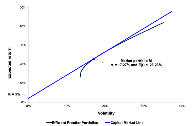
In the case of risky assets only, the efficient frontier (the set of optimal portfolios) is represented below in Figure 1.

Figure 1. Efficient frontier with risky assets only.
img_Simtrade_CML_graph_1
Source: Computation by the author.

Risky assets and a risk-free asset

In the case of risky assets and a risk-free asset, the efficient frontier (the set of optimal portfolios) is represented below in Figure 2. In this case, the efficient frontier is a straight line called the Capital Market Line (CML).

Figure 2. Efficient frontier with risky assets and a risk-free asset.

Source: Computation by the author.

The CML joins the risk-free asset and the tangency portfolio, which is the intersection with the efficient frontier with risky assets only. We can reasonably conclude from Figure 2 that, to increase expected return, an investor has to increase the amount of risk he or she takes to attain returns higher than the risk-free interest rate. As a result, the Sharpe ratio of the market portfolio equals the slope of the CML. If the Sharpe ratio is more than the CML, an investment strategy can be implemented, such as buying assets if the Sharpe ratio is greater than the CML and selling assets if the Sharpe ratio is less than the CML (Drake and Fabozzi, 2011).

Investors who allocate their money between a riskless asset and the risky market portfolio M can expect a return equal to the risk-free rate plus compensation for the number of risk units σ_P) they accept. This result is in line with the underlying notion of all investment theory: investors perform two services in the capital markets for which they might expect to be compensated. First, they enable someone else to utilize their money in exchange for a risk-free interest rate. Second, they face the risk of not receiving the promised returns in exchange for their invested capital. The term E(r_M)- R_f) / σ_M refers to the investor’s expected risk premium per unit of risk, which is also known as the expected compensation per unit of risk taken.

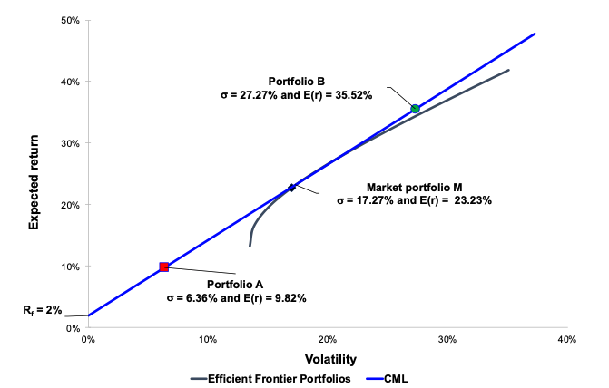
Figure 3 represents the Capital Market Line which connect the risk-free asset to the efficient frontier line. The straight line in Figure 3 represents a combination of a risky portfolio and a riskless asset. Any combination of the risk-free asset and Portfolio A is similarly outperformed by some combination of the risk-free asset and Portfolio B. Continue drawing a line from R_f to the efficient frontier with increasing slopes until you reach Portfolio M’s point of tangency. All other possible portfolio combinations that investors could build are outperformed by the collection of portfolio possibilities along Line R_f-M, which is the CML. The CML, in this sense, represents a new efficient frontier that combines the Markowitz efficient frontier of risky assets with the ability to invest in risk-free securities. The CML’s slope is (E(r_M)- R_f) / σ(_M), which is the highest risk premium compensation that investors can expect for each unit of risk they take on (Reilly and Brown, 2012) (Figure 3).

If we fully invest our cash on the risk-free rate, we would be exactly on the y axis with an expected return of 2%. Each time we move along the curve that connects the risk-free rate to the optimum market portfolio, we allocate less weight to the risk-free rate, and we overweight more on riskier assets (Point A). Points M represents the optimal risky portfolio in the efficient frontier line, which minimizes the overall portfolio variance. It would have a weighting of 45% in stock A and a 55% in stock B, which would offer a 26.23% annualized return for a 17.27% annualized volatility. Point B represents a portfolio composition that is based on a leveraged position of 140% on the optimal risky portfolio and a short position on the risk-free asset of -40% (Figure 3).

Figure 3. Efficient frontier with different points.

Source: Computation by the author.

Mathematical representation

We can define the CML as the line that is tangent to the efficient frontier which connects the risk-free asset with the market portfolio:

img_SimTrade_CML_equations_0

Where:

σ_P: the volatility of portfolio P
R_f: the risk-free interest rate
E(R_M): the expected return of the market M
σ_M: the volatility of the market M
E[R_M– R_f]: the market risk premium.

The expected return of the portfolio can be computed as:

img_SimTrade_CML_equations_1

The Sharpe Ratio is shown in parenthesis, and it compares the performance of an investment, such as a security or portfolio, to the performance of a risk-free asset after adjusting for risk. It is calculated by dividing the difference between the investment returns and the risk-free return by the standard deviation of the investment returns. It denotes the additional amount of return that an investor receives for each unit of risk increase (Sharpe, 1963). We can define it mathematically as:

img_SimTrade_CML_equations_2

We can identify the following relationship between the slope of the CML and the Sharpe ratio of the market portfolio, defined mathematically as follows:

img_SimTrade_CML_equations_3

A simple strategy for stock selection is to buy assets with Sharpe ratios that are higher than the CML and sell those with Sharpe ratios that are lower. Indeed, the efficient market hypothesis implies that beating the market is impossible. As a result, all portfolios should have a Sharpe ratio that is lower than or equal to the market. As a result, if a portfolio (or asset) has a higher Sharpe ratio than the market, this portfolio (or asset) has a higher return per unit of risk (i.e. volatility), which contradicts the efficient market hypothesis. The alpha is the abnormal excess return over the market return at a given level of risk.

Why should I be interested in this post?

Sharpe ratio is a popular tool for assessing portfolio risk/return in finance. The Sharpe ratio informs the investor precisely which portfolio has the best performance among the available options. This simplifies the investor’s decision-making process. The higher the ratio, the greater the return for each unit of risk.

If you are a business school or university undergraduate or graduate student, this content will help you in broadening your knowledge of finance.

Useful resources

Academic research

Pamela, D. and Fabozzi, F., 2010. The Basics of Finance: An Introduction to Financial Markets, Business Finance, and Portfolio Management. John Wiley and Sons Edition.

Lintner, J. 1965a. The Valuation of Risk Assets and the Selection of Risky Investments in Stock Portfolios and Capital Budgets. The Review of Economics and Statistics 47(1): 13-37.

Lintner, J. 1965b. Security Prices, Risk and Maximal Gains from Diversification. The Journal of Finance, 20(4): 587-615.

Mossin, J. 1966. Equilibrium in a Capital Asset Market. Econometrica, 34(4): 768-783.

Reilly, R. K., Brown C. K., 2012. Investment Analysis & Portfolio Management, Tenth Edition.

Sharpe, W.F. 1963. A Simplified Model for Portfolio Analysis. Management Science, 9(2): 277-293.

Sharpe, W.F. 1964. Capital Asset Prices: A Theory of Market Equilibrium under Conditions of Risk. The Journal of Finance, 19(3): 425-442.

About the author

The article was written in November 2021 by Youssef LOURAOUI (Bayes Business School, MSc. Energy, Trade & Finance, 2021-2022).

Active Investing

November 20, 2021 by Youssef LOURAOUI

In this article, Youssef LOURAOUI (Bayes Business School, MSc. Energy, Trade & Finance, 2021-2022) elaborates on the concept of active investing, which is a core investment strategy that relies heavily on market timing and stock picking as the two main drivers of financial performance.

This article is structured as follows: we introduce the concept of active investing in asset management. Next, we present an overview of the academic literature regarding active investing. We finish by presenting some basic principles on active investing.

Introduction

Active investing is an approach for going beyond matching a benchmark’s performance and instead aiming to outperform it. Alpha may be calculated using the CAPM framework, by comparing the fund manager’s expected return with the expected market return (Jensen, 1968). The search for alpha is done through two very different types of investment approaches: stock picking and market timing.

Stock picking

Stock picking is a method used by active managers to select assets based on a variety of variables such as their intrinsic value, the growth rate of dividends, and so on. Active managers use the fundamental analysis approach, which is based on the dissection of economic and financial data that may impact the asset price in the market.

Market timing

Market timing is a trading approach that involves entering and exiting the market at the right time. In other words, when rising outlooks are expected, investors will enter the market, and when downward outlooks are expected, investors will exit. For instance, technical analysis, which examines price and volume of transactions over time to forecast short-term future evolution, and fundamental analysis, which examines the macroeconomic and microeconomic data to forecast future asset prices, are the two techniques on which active managers base their decisions.

Review of academic literature on active investing

As fund managers tried strategies to beat the market, financial literature delved deeper into the mechanism to achieve this purpose. Jensen’s groundbreaking work in the early ’70s gave rise to the concept of alpha in the tracking of a fund’s performance to distinguish between the fund’s manager’s ability to generate abnormal returns and the part of the returns due to luck (Jensen, 1968).

Jensen develops a risk-adjusted measure of portfolio performance that quantifies the contribution of a manager’s forecasting ability to the fund’s returns. He used the measure to quantify the predictive ability of 115 mutual fund managers from 1945 to 1964—that is, their ability to produce returns above those expected given the risk level of each portfolio.

Not only does the evidence on mutual fund performance indicate that these 115 funds on average were unable to forecast security prices accurately enough to outperform a buy-and-hold strategy, but there is also very little evidence that any individual fund performed significantly better than what we would expect from mutual random chance. Additionally, it is critical to highlight that these conclusions hold even when fund returns are measured net of management expenses (that is assume their bookkeeping, research, and other expenses except brokerage commissions were obtained free). Thus, on average, the funds did not appear to be profitable enough in their trading activity to cover even their brokerage expenses.

Core principles of active investing

First principle: market efficiency varies between asset classes.

Investment information is not always readily available in all markets. For less efficient asset classes, an “active” management strategy offers a larger possibility to outperform the market, whereas a “passive” investment strategy may be more appropriate for highly efficient asset classes. In other words, there are compelling advantages for incorporating both active and passive techniques into an overall portfolio.

For example, Wall Street analysts cover a huge portion of US large size shares, making it harder to locate cheap companies. For this highly efficient asset class, a passive investment strategy may be more cost-effective in some cases. On the other side, emerging market equities are sometimes under-researched and difficult to appraise, providing an active manager with additional opportunities to identify mispriced companies. The critical point here is to notice the distinctions and then make the appropriate decisions.

Second principle: market efficiency varies across asset classes.

Within practically every asset class, active and passive management strategies can alternate as winners periodically. Even the most efficient asset classes can occasionally benefit from active management over passive. The reason is substantially distinct from the one stated in Principle One. Principle Two is related to the “Grossman-Stiglitz Paradox”: If markets are fully efficient, there is no reason to investigate them; yet markets can only be perfectly efficient for as long as they are regularly investigated. When investors run out of patience researching stocks in a highly efficient market, passive investment becomes appealing, reopening the door to opportunities for active research. This can result in an annual cycle of active/passive trends.

In some investing environments, active strategies have tended to benefit investors more, while passive strategies have tended to outperform in others. For instance, active managers may outperform more frequently than passive managers when the market is turbulent, or the economy is deteriorating. On the other way, when certain securities within the market move in lockstep or when stock valuations are more consistent, passive strategies may be preferable. Investors may gain from combining passive and active strategies in a way that exploits these insights, depending on the opportunity in various areas of the capital markets. Market conditions, on the other hand, vary constantly, and it frequently takes an intelligent eye to determine when and how much to skew toward passive rather than active investments (Morgan Stanley, 2021).

It’s worth noting that attaining consistently successful active management has historically been more challenging in some asset classes and segments of the market, such as large US company stocks. As a result, it may make sense to be more passive in certain areas and more active in asset classes and segments of the market where active investing has historically been more rewarding, such as overseas stocks in emerging markets and smaller U.S. corporations (Morgan Stanley, 2021).

Why should I be interested in this post?

If you are a business school or university undergraduate or graduate student, this content will help you in broadening your knowledge of finance.

Useful resources

Academic research

Grossman, S., Stiglitz, J., 1980. On the impossibility of Informationally efficient markets. The American Economic Review, 70(3), 393-408.

Lintner, J. 1965a. The Valuation of Risk Assets and the Selection of Risky Investments in Stock Portfolios and Capital Budgets. The Review of Economics and Statistics 47(1): 13-37.

Lintner, J. 1965b. Security Prices, Risk and Maximal Gains from Diversification. The Journal of Finance, 20(4): 587-615.

Mangram, M.E., 2013. A simplified perspective of the Markowitz Portfolio Theory. Global Journal of Business Research, 7(1): 59-70.

Markowitz, H., 1952. Portfolio Selection. The Journal of Finance, 7(1): 77-91.

Mossin, J. 1966. Equilibrium in a Capital Asset Market. Econometrica, 34(4): 768-783.

Sharpe, W.F. 1963. A Simplified Model for Portfolio Analysis. Management Science, 9(2): 277-293.

Sharpe, W.F. 1964. Capital Asset Prices: A Theory of Market Equilibrium under Conditions of Risk. The Journal of Finance, 19(3): 425-442.

Business analysis

Forbes, 2021. Active or Passive investing? Two principles provide the answer

JP Morgan Asset Management, 2021. Investing

Morgan Stanley, 2021. Active vs Passive management

About the author

The article was written in November 2021 by Youssef LOURAOUI (Bayes Business School, MSc. Energy, Trade & Finance, 2021-2022).

Social trading

November 19, 2021 by Daksh GARG

Social trading

In this article, Daksh GARG (ESSEC Business School, Master in Strategy & Management of International Business (SMIB), 2020-2021) explains how social networks and online communities have led to emergence of new way of trading called social trading. This article answers the following questions: What is social trading? What are the platforms on which social trading is being done? And what are some of the potential disadvantages of putting your money and following the trend of social trading?

What is social trading?

Social trading in the stock market uses the wisdom of the online community to develop strategies and portfolios that best fit the investment needs of the community members.

Social trading is security trading on a digital platform where investors derive their investment decisions from information or signals provided by other traders in the community. Social trading enables experienced retail investors to share their investments strategies or portfolios with the online community. It provides the opportunity to observe the ideas and to discuss, comment or even copy them. The concept of social trading combines the investment ideas of traders with a leader follower principle. The star traders are called signal providers. They share their investment ideas with the online community. Members of the community execute their strategies and portfolios in a real money account or in a virtual account where no real funds are at risk. This is illustrated in Figure 1.

Figure 1. Social trading: interaction between the experienced trader and social traders.

Source: IG

What do you need to know before you start social trading?

Social trading has removed the barriers to financial inclusion, but it is also said to downplay a lot of the knowledge required to negotiate in financial markets. One of the largest faults a social trader can make is thinking it is risk free. All trading involves risk, and traders are likely to make a loss at one point or another. The idea of trusting a judgement of third person – while retaining all the risk of loss – is seen as a large drawback of social trading. Financial markets require knowledge and patience, and social trading can potentially help you skip a few steps, but it does so at the expense of experience. You might take on some other persons, but you implement plan should be unique to you and your aims. Although the strategies of others can be used to create some guidance for your trades, their plans will be suited to their own goal. Each individual perceives risk differently so, so trading the way someone else would isn’t always necessarily a good idea.

How to get started with social trading?

Select a social trading platform/broker

There are a lot of different platforms available in the market. But make sure the platform provides all of the functions you want to enable you to utilize it successfully and is trustworthy.

Select and research the traders you want to learn and copy from

The platforms will provide you with recommendations of traders that you can copy and learn from, but it is essential to do your own research. Research the markets they trade, the strategies they use and the risk parameters. Do your due diligence.

Allocate a set amount to each trader

Allocate a portion of your capital to each trader you follow. Think of this as your risk management. You will have researched the trader you are tracking, and now it’s about diversifying your investment into each trader. For traders with a high-risk strategy, you may want to allocate less money to traders with a lower risk strategy.

Figure 2 gives some of the popular social trading platforms emerged in past few years.

Figure 2. Popular social trading platforms.

Source: www.diaman.eu/blog

Why should I be interested in this post?

Investing in financial markets such as stocks, foreign exchange (forex) and cryptocurrencies requires extensive knowledge and experience. You need to be up to date with news events affecting the business world, and also have the capability of reading charts, analytics reports and understand trends. If you lack this capacity, chances are you may lose your money in the market. Social trading platforms might come in handy in this phenomenon, but you should always be careful and aware of the risks. This article provides a good introduction who is starting their journey in social trading.

Useful resources

IG Social trading explained Accessed November 2, 2021.

CMC markets Social trading Accessed November 2, 2021.

About the author

The article was written in November 2021 by Daksh GARG (ESSEC Business School, Master in Strategy & Management of International Business (SMIB), 2020-2021).

Use of AI in investment banking

November 19, 2021 by Daksh GARG

Use of AI in investment banking

In this article, Daksh GARG (ESSEC Business School, Master in Strategy & Management of International Business (SMIB), 2020-2021) explains how the use of AI is transforming the investment banking industry.

What is artificial intelligence?

Artificial intelligence (AI) generally refers to the ability of machines to exhibit human-like intelligence and a degree of autonomous learning. An example could be training machines to recognize patterns and solve complex problems by analyzing those patterns.

Recently there has been a push to work with AI in the investment industry. The conditions to do so are optimal now, or at least more so than in the past. There have great leaps in computer processing abilities, allowing the cost of quality processing tech to decrease. There has also been a sharp increase in the availability of accessible data, which AI can use as needed. This has led to AI being cost effective enough to be used in carrying out investment guidance and analysis.

When can AI add value?

There have been several implementations of AI across the broad spectrum of investment banking , and the rapid pace of adoption paves the way for greater efficiencies in almost all departments and functions. AI has the potential to completely transform the competitive dynamics given its indispensability in investment banking. Much like a chain reaction, investment banks will adopt AI if even one of their peers adopts it, and they already have. This will keep going until all of them rely on the accuracy and effectiveness of AI in their daily trade and investment making decisions. By its very nature, investment banking is a highly competitive industry, and intelligent tools can augment every facet from trade processing to defining structured products and projecting returns on capital, simulating market conditions to support accurate and fast decision making, to even improving the customer experience. AI will also enhance back-office functions, ensuring quicker and easier settlements with minimal human error.

Figure 1. Use of Artificial intelligence / Machine learning AI/ML deployment across various components of financial services industry.
Use of AI/ML in financial services industry.

Use of AI/ML in financial services industry.

Source: Refinitiv AI/ML survey August 2020

Some current use cases

There are several use cases already being adopted for use of AI and ML in the financial services industry. Some of the prominent examples of companies using AI are:

ING

ING leverages the power of AI to empower bond traders make faster and more accurate pricing decisions, with Katana, an AI tool that uses predictive analytics to ensure traders are quoting the right price when buying and selling bonds for their clients, based entirely on historic and real-time streaming data.

Barclays

The UK investment bank takes its AI initiatives very seriously, with the whole subsidiary dedicated to making the investment bank’s vision of becoming “the most AI savvy workforce in the UK” come true. Payments and trade decisions for their short term structured products are handled by their in-house AI.

UBS

UBS uses machine learning and neural networks for facilitating accurate decision making of its traders on the floor, including the allocation of funds and analyzing real time data to enhance the performance of its high performing traders.

JP Morgan Chase

The American investment banking giant is using AI to interpret loan agreements. As a part of its AI agenda, its now famous Contract Intelligence AI system saved 360,000 hours of mundane work, interpreting and recording contract clauses, freeing up support staff to focus on high value delivery.

Figure 2. Potential use cases of AI in various components of investment banking.

Source: Refinitiv AI/ML survey August 2020

The challenges towards wide-spread adoption of AI in investment baking

We cannot assume that AI will replace analysts anytime soon. There are a lot of nuanced human interactions and decisions for the machines to acquire at their current development phase. At this stage in the AI managing processes, leading analysis, and making judgment calls can be very dangerous. Like humans, the machines have to follow training for some time before performing as they are designed. Human supervision on these systems will be essential. After the collapse of many banks in 2008 there has been a wide spread adoption of AI. We are talking about more effective gathering data, from hours to mere seconds. Artificial Intelligence enables investment bankers to focus more on the transactions rather than the immense piles of hard work. There are certain costs towards adoption and a potential job loss also. In 2000, Goldman Sachs’ cash equities trading desk was holding 600 traders. Today, only two traders are left on the desk with machines doing the heavy lifting of the work.

Conclusion

Banks are automating their processes day by day. Despite the increasing and better application of AI in banking and financial industry contributing towards innovation, its adoption in the industry is still at the stage of infancy. Low level of maturity, infrastructure, reluctant industry adoption, increased technical complexity and high costs are the major reasons preventing financial services firms for large scale adoption. But this would change in future.

Why should I be interested in this post?

Artificial Intelligence is emerging in the digital era that we know now, expected to be the next big thing. This article shows the benefits and challenges of AI in the investment banking industry.

Useful resources

McKinsey (19/09/2020) AI-bank of the future: Can banks meet the AI challenge? Accessed November 2, 2021.

Forbes (31/10/2020) The State Of AI Adoption In Financial Services Accessed November 2, 2021.

About the author

The article was written in November 2021 by Daksh GARG (ESSEC Business School, Master in Strategy & Management of International Business (SMIB), 2020-2021).

The IRR, XIRR and MIRR functions in Excel

June 4, 2024November 19, 2021 by Léopoldine FOUQUES

The IRR, XIRR and MIRR functions in Excel

In this article, Léopoldine FOUQUES (ESSEC Business School, Global Bachelor of Business Administration, 2017-2021) presents the IRR function in Excel to compute the internal rate of return of a series of cash flows.

About Excel

Excel is by far the most used financial modeling tool across the world to build models and perform analysis. Knowing which Excel function to use can help employees in the financial sector (financial analysts, fund managers, risk managers, traders, etc.) to work faster and build a more powerful model.

The internal rate of return (IRR)

Definition

The computation of the internal rate of return (IRR) is based on the net present value (NPV) of an investment. In financial modelling, an investment is represented by a series of cash flows: CF₀, CF₁, CF₂, …, CF_T. For a classic investment, the first cash flow, CF₀, is negative (outflow) and the future cash flows, CF₁, CF₂, …, CF_T are positive (inflows).

The net present value (NPV) of an investment is computed according to the following formula:

where r is the discount rate that takes into account the risk of the project.

The IRR corresponds to the value of the discount rate for which the NPV is equal to 0:

The IRR is the solution of a non-linear equation:

Use in finance

One of the most important functions is the Internal Rate of Return (IRR) function, as it’s an easy function to compare an investment’s return, based on a series of cash flows.

The function is very useful in financial modeling. Indeed, it’s frequently used to compare scenarios before deciding about a project. An example is when a company is presented with two opportunities: one is investing in a new factory and the second is expanding its existing factory.

By using IRR, we can estimate the IRR for each scenario and verify which one is higher than the average cost of capital of the business (the Weighted Average Cost of Capital or WACC) is a calculation of a firm’s cost of capital in which each category is proportionally weighted).

The Excel functions to compute the IRR

Building a math-based calculation is time-consuming and complicated, so Excel offers three functions for the calculation of the internal rate of return: IRR, MIRR, and XIRR.

The IRR function

The IRR function uses one required argument and one optional:

The values: they represent the series of cash flows, including net income value and investments.
The guessed number for the expected internal rate of return. If omitted, the function will default to 0.1 (= 10%).

You can download the Excel file below in which I illustrate the use of the IRR function in Excel based on a simple example.

Note that the IRR corresponds to a period rate. Monthly cash flows lead to a monthly IRR, quarterly cash flows lead to a quarterly IRR; and annual cash flows lead to an annual IRR. As, in practice, the standard is to work annual rates, monthly and quarterly IRR have to annualized.

Note that the use of the IRR function assumes that the period between each cash flow is the same (equal-size payment periods), for example one year.

From the IRR function to the XIRR function

If the period between each cash flow is not the same, the IRR function should not be used. It is the case with monthly cash flows as the months of the year may contain 28, 29, 30 or 31 days.

In this case, the XIRR function comes into play to calculate a correct internal rate of return, taking into consideration the periods of different sizes.

The XIRR function has three arguments:

The values
The dates for cash outflows and inflows.
The guessed number for the expected internal rate of return (optional argument).

You can download the Excel file below in which I illustrate the use of the IRR and XIRR functions in Excel based on a simple example.

From the IRR function to the MIRR function (Modified Internal Rate of Return)

The MIRR function is quite the same as the IRR function, except that it takes into consideration both the cost of borrowing the initial investment funds (discount rate) and reinvestment rates for future cash flows.

In contrast to IRR, MIRR assumes that cash flows from a project are reinvested at the firm’s cost of capital (rate of return on a portfolio company’s existing securities).

To compute the MIRR, the Excel function uses the following parameters:

The values
The guessed number for the expected internal rate of return (optional argument).
The financial rate: the finance rate of interest paid
The reinvest rate: the interest rate earned from the reinvested profit

Where FV represents the Future Value of positive cash flows at the cost of capital for the company, PV represents the Present Value of negative cash flows at the financing cost of the company, and T represents the number of periods.

You can download the Excel file below in which I illustrate the use of the IRR and MIRR functions in Excel based on a simple example.

Some of the accountants say that the MIRR function is less valid than the other because not all the flows are reinvested fully. Although we can use a less important interest rate to compensate the partial investment; but we think the best approach will be the inclusion of the three calculations (IRR, XIRR, and MIRR).

Limits of the IRR

The non-linear equation for obtaining the IRR may have one solution, several solutions or no solution according to the sequence of cash flows. These represent limits of the IRR as an investor would like one value when estimating its investment.

Another limit of the IRR as a decision criterion for investing is that the result is not in agreement with the decision criterion based on NPV, which represents the value created by the investment.

You can download the Excel file below in which I provide an example to illustrate the limit of the IRR when selecting investment when two projects are available.

Useful resources

Mazars Excel IRR Function And Other Ways To Calculate IRR In Excel

About the author

The article was written in November 2021 by Léopoldine FOUQUES (ESSEC Business School, Global Bachelor of Business Administration, 2017-2021).

My experience as Consultant in Energy & Utilities at Atos Worldgrid

November 19, 2021 by Léopoldine FOUQUES

My experience as Consultant in Energy & Utilities at Atos Worldgrid

In this article, Léopoldine FOUQUES (ESSEC Business School, Global Bachelor of Business Administration, 2017-2021) shares her experience as Consultant in Energy & Utilities at Atos Worldgrid.

About Atos Worldgrid

Founded in 1997, Atos is a French multinational firm specialized in information technology (IT), headquartered in Bezons, France. Member of the CAC 40 index, Atos has been positioned as a leader in cloud infrastructure, cybersecurity, and super calculator and operates in 71 countries.

As a leader in digital transformation, Atos supports its customers in large-scale industrial projects and covers a wide range of sectors: financial services and insurance, healthcare, manufacturing, public sector and defense, resources and services, and telecommunications and media.

Since 2010, Atos has specialized in a secure and decarbonized digital through the brand “Atos Worldgrid”. The purpose of Worldgrid is to offer an extensive ecosystem of technology partners and implement critical Information technology / Operational technology (IT/OT) convergence projects. It provides services along the entire energy value chain to over 250 clients worldwide, operating all the energy sources, as oil & gas, biofuels, wind, solar, sea, hydro, coal, and nuclear, and covers all the distributed grid, from the generation to the retail.

My experience at Atos

My interest in the technology field was further intensified during my studies at ESSEC by following the course on blockchain and big data. That is why I came to work for Atos, a leading IT group in the digital transition, for a two-year apprenticeship.

Working as Consultant in Energy & Utilities in the Atos Worldgrid entity, I became aware of the interest of science applied to ecology to address current challenges, particularly those related to the digital and energy transition. During this apprenticeship, I became familiar with a complex and fast-moving environment. I put into practice what I had learned since the beginning of my studies and contributed to many projects with a proven innovative dimension. Thus, I had the opportunity to work on a wide variety of missions. In particular, I conducted several studies on the energy sector, contributed to the design of commercial offers for startups, and developed a platform, in partnership with Méteo-France. These missions allowed me to put into practice my managerial qualities and my customer orientation. On the other hand, my curiosity, and my appetite for the subjects I studied led me to work on information systems and asset management for companies in the energy and utility sector.

Why is necessary to put digital into the energy sector?

Atos is one of the leaders in services for Smart Cities (intelligent and connected cities). The enterprise has a wide range of solutions for cities and local authorities, covering consulting, systems implementation, user-centered design and managed services.

During my internship I had the opportunity to work on many subjects that are part of Smart Cities projects. Furthermore, I became aware that digital was at the heart of all transformation projects.

For many actors, the Smart City will be the “natural” environment of the improved human being. Therefore, we intend to provide the city with digital knowledge and technologies. Faced with the need for a change in ecological strategy, the value of new technologies is becoming increasingly important in discussions. The conjunction of ecology and IT was also widely discussed at the Davos Economic Forum in January 2020. It is in this context that Big Data initiatives have multiplied.

In the emerging context of Smart Cities or connected cities in which uses are rethought and resources are optimized, Big Data is becoming increasingly important. Indeed, faced with the exponential volume of data produced by various actors, controlling it becomes an essential tool that cities must appropriate. The data would enable the development of new services for the city, optimize existing ones and reconcile citizens’ expectations with current policies. Finally, is the central element of the most innovative projects, and constitute most city modernization projects. These technologies open the door to new conjunctures and represent the foundation stone of the cities of tomorrow.

The valorization of this data is one of the main challenges for territories and leads to the rethinking of new tools. Thanks to the mass of data that can be collected, both public and private players can anticipate future innovations and developments and thus lead the city towards a sustainable and responsible approach. The use cases are many and are very often based on the triptych: mobility, energy management and street services, i.e. services for both local or national authorities and consumers.

At the heart of the connected city, the smart energy grids must learn to be resilient.

In order to succeed in the energy transition, the electricity system is undergoing considerable change: development of renewable energies, deployment of electric vehicles, the emergence of new use cases, etc. To facilitate this transition, the energy grid must become more efficient. But the smart grid is not born smart, it becomes smart. Atos Worldgrid aims to make its cities a reality. The solutions support governments in their mission to provide intelligent integrated services to their citizens and economic partners.

In 2010, The French Parliament adopted the Law on National Commitment for the Environment : The Grenelle II Law. The Grenelle II law includes energy and climate concerns in the French objectives, with the aim of reducing consumption and greenhouse gas emissions. In addition, the law accelerates the deployment of renewable energy. Among other things, the state is committed to building at least 500 wind turbines per year.

Faced with this development of natural energies, the question of grid stability becomes essential. Indeed, these weather-sensitive energies are not predictable, and a bad estimate of the production can lead to very strong price fluctuations and a shortage of energy. The renewable energy produced must be estimated accurately to avoid a large gap between the energy produced and the energy sold, as the energy produced is not linear. A financial imbalance has repercussions on the whole value chain, from producer to final consumer. To prevent producers from producing too much or too little or aggregators from disturbing the balance of the grid by buying too much or too little, tools must be designed. This is the main challenge for companies like Atos and to achieve a transition to renewable energy.

Source: Wikimedia

At the heart of these smart grids and this revolution, the deployment of smart meters, such as Linky, developed by Atos, is today an essential building block for the success of this transition. Installed directly in French homes, it measures the daily electricity consumption of the home and transmits this data to the network operator. Its advantages are numerous. Firstly, its scope is ecological since it facilitates the insertion of renewable energy sources into the energy network. By collecting information on household consumption, renewable energies are better distributed and optimized, which contributes to the flexibility and therefore the stability of the network. Also, the consumer is also more widely integrated into the process. With smart grids, it is consumption that adapts to production and thus gives the consumer a new role. The Linky smart meter is an essential building block in this logic.

To support the energy transition and encourage the massive integration of renewable energy sources and new uses of mobility, network infrastructures have had to adapt quickly. In addition to the new dimensioning of the network, which has become a smart grid, the digitization functions resulting from Big Data have provided optimization and control tools for better operational performance. These advanced models have made it possible to improve the observability and controllability of the network, for better control of renewable energy connections. Atos is active in this area. In collaboration with Méteo France, It has developed service platform that uses Machine Learning algorithms to estimate the production of renewable energy in detail.

What I learned during my internship

During my work placement I acquired certain consulting skills, and I also learned to work in a team and to manage teams, to lead working groups. I have acquired both managerial and technical skills.

Above all, I discovered a sector that was totally unknown to me. As I progressed in the missions, I became familiar with a specialized vocabulary and gradually understood the technical workings. This experience in a digital services company was very enriching, both personally and professionally, and gave me the desire to continue in this direction.

Useful resources

smartgrids Introduction aux smart grids

European Commission Smart grids and meters

European Commission Energy modelling

About the author

The article was written in November 2021 by Léopoldine FOUQUES (ESSEC Business School, Global Bachelor of Business Administration, 2017-2021).

Bollinger Bands

November 18, 2021 by Jayati WALIA

Bollinger Bands

In this article, Jayati WALIA (ESSEC Business School, Grande Ecole Program – Master in Management, 2019-2022) presents the popular Bollinger bands used in technical analysis.

This post is organized as follows: we introduce the concept of Bollinger bands and provide an illustration with Apple stock prices. We delve into the interpretation of Bollinger bands as port and resistance price levels used to define buy and sell trading signals. We then present the techniques to compute the Bollinger bands and finally discuss their limitations.

Introduction

In the 1980s, John Bollinger, a long-time market technical analyst, developed a technical analysis tool for trading in securities. At that time, it was presumed that volatility was a static quantity, a property of a security, and if it changed at all, it would happen in a long-term period. After some experimentation, Bollinger figured that volatility was indeed a very dynamic quantity and a moving average computed on a time period (typically 20 days) with bands drawn above and below at intervals could be determined by a multiple of standard deviation.

Unlike a percentage calculation from a simple moving average, Bollinger bands simply add and subtract a standard deviation (or a multiple of the standard deviation, usually two). The tool thus represents the volatility in the prices of the security which is measured by the standard deviation of the prices of the security. The bands are used to understand the overbought or oversold levels for a security and to follow the price trends. The indicator/tool comprises of three main bands, an upper band, a lower band, and a middle band.

The middle band is a simple moving average (SMA), which is usually computed over a rolling period of 20 trading days (about a calendar month). The upper and the lower bands are positioned two standard deviations away from the SMA. The change in the distance of the upper and lower bands from the SMA determine the price strength (which is the strength of price trend of stock relative to overall market trend) and the lower and the upper levels for the stock prices. Bollinger bands can be applied to all financial securities traded in the market including equities, forex, commodities, futures, etc. They are used in multiple time frames (daily, weekly and monthly) and can be even applied to very short-term periods such as hours.

Figure 1 represents the evolution of the price of Apple stocks with the Bollinger bands for the period January 2020 – September 2021.

Figure 1. Bollinger bands on Apple stock.
Bollinger bands Apple stock
Source: computation by the author (data source: Bloomberg).

Figure 2 illustrates for the price of Apple stocks the link between the Bollinger bands and volatility measured by the standard deviation of prices. The lower the volatility, the narrower the bands.

Figure 2. Bollinger’s bands and volatility
Bollinger bands and volatility Apple stock
Source: computation by the author (data source: Bloomberg).

How to interpret Bollinger bands

Traders use the Bollinger bands to determine the strength of the price trend of a stock. The upper and lower bands measure the degree of volatility in prices over time. The width between the bands widens as the volatility in the stock prices increases and indicates a strong trend in the price movement. Conversely, the width between the bands narrows as the volatility decreases, indicating that the price of the security is range-bound. When this width is extremely narrow and contracting, it indicates that there can be a potential breakout in the price movement soon and is referred to as “Bollinger squeeze”. If the price crosses the upper band, it may indicate that the movement will be in an uptrend, and If the price crosses the lower band, it may indicate that the movement will be in a downtrend.

If the price hits the upper band, it indicates an overbought level in the security, and when the price hits the lower band, it indicates an oversold level. When the price crosses the upper band, traders consider it to a positive signal to buy the stock as the price trend is in an upward direction and shows great strength. Similarly, when the price crosses the lower band, traders consider it to a positive signal to sell the stock as the price trend is in a downward direction and shows great strength.

In other words, Bollinger bands act as dynamic resistance and support levels for the price of the security. Thus, once prices touch either of the upper or lower band levels, they tend to return back to the middle of the band. This phenomenon is referred to as the “Bollinger bounce” and many traders rely extensively on this strategy when the market is ranging and there is no clear trend that they can identify.

Calculation

The three bands of the Bollinger bands are calculated using the following formula:

Middle Band

The middle band is the simple moving average (SMA) over a 20-day rolling period. To calculate the SMA, we compute the average of the closing prices of the stock over the past 20 days.

SMA 20 days

To compute the upper and lower bands, we need first to compute the standard deviation of prices.

img_std_dev_bollinger_bands

Upper band

The upper band is calculated by adding the SMA and the standard deviation times two:

Bollinger upper band

Lower band

The lower band is calculated by subtracting the standard deviation times two from the SMA:

Bollinger lower band

Limitations of Bollinger bands

Bollinger bands are considered to be lagging indicators since they represent the simple moving average which is based on the historical stock prices. This means that the indicator is not very useful in predicting the future price patterns as the indicator signals a price trend when it has already started to happen.

To benefit from the Bollinger bands, traders often combine this indicator with other technical tools like the Relative Strength Index (RSI), Stochastic indicators and Moving Averages Convergence-Divergence (MACD).

▶ Jayati WALIA Trend Analysis and Trading Signals

▶ Jayati WALIA Moving averages

▶ Jayati WALIA Standard deviation

Useful resources

Bollinger bands

Fidelity: Technical Indicators: Bollinger Bands

About the author

The article was written in November 2021 by Jayati WALIA (ESSEC Business School, Grande Ecole Program – Master in Management, 2019-2022).

Trend Analysis and Trading Signals

November 18, 2021 by Jayati WALIA

Trend Analysis and Trading Signals

In this article, Jayati WALIA (ESSEC Business School, Grande Ecole Program – Master in Management, 2019-2022) presents an overview of trend analysis and trading signals in stock price movements.

This post is organized as follows: we introduce the concept of trends used in technical analysis and its link with support and resistance price levels used to define buy and sell trading signals. Then, we present the different types of trends and discuss the time frame for their analysis. Trends based on straight lines, moving averages and the Fibonacci method are presented in detail with examples using Moderna, Intel, Adobe and Apple stock prices.

Introduction

Trend Analysis is one of the most important areas of technical analysis and is key to determining the overall direction of movement of any financial security. The analysis of trends in asset prices is used to find support and resistance price levels and in fine generate buy and sell trading signals when these support and resistance price levels are broken.

Support and resistance

The support and resistance are specific points on the price chart of any security which can be used to identify trade entry and exit points. The support refers to the price level at which price generally bounces upwards and buying trend is strongest. Likewise, the resistance price is a price level at which selling power is strongest and the price of the security struggles to break above the resistance. The support and resistance levels can act as potential entry and exit points for any trade since it is at these levels that the price can either “break-out” of the current trend or continue moving in the same direction. The support and resistance can be determined by using prices or Japanese candlesticks.

Ways to define trends

The two main ways to define trends in financial markets are straight lines and moving averages. Straight lines simply give static support and resistance levels that do not change over time. Moving averages give dynamic support and resistance levels that are continuously adjusted over time. Another popular method to define trends is the Fibonacci method.

Trends based on straight lines

Overview

Trend lines are indicators to identify the trends in the price chart of a security within a time frame (say one week or one month). Trend analysis using trend lines takes specific price levels or zones that correspond to support and resistance. An uptrend is based on the principle of higher highs and higher lows; similarly, a downtrend is based of lower highs and lower lows.

These price levels are the major zones where the market seems to respond by making a strong advance or decline. If the stock prices are in an uptrend, it shows an increasing demand for the stock and if the stock prices are in downtrend, it shows an increasing supply for the stock.

Trend lines can be built by connecting two or more prices (peaks or troughs) in either direction of a stock price movement on a time frame determined by the trader (1 hour, 1 day, 1 week, etc.) over a period (3 months, 6 months, 12 months, etc.). For a trend line to be valid, a minimum of two highs or lows should be used. The more times price movement touches a trend line, the more accurate is the trend indicated by the line.

Different types of trends using straight lines

The use of market trends in technical analysis in financial markets is based on the concept that past movements in the prices of the stock provides an overview of the future movement. Note that such an approach is in contradiction with the Market Efficiency Hypothesis (EMH) developed by Fama (1970), which states that the best prediction of the price of tomorrow is the price of today (past prices being useless).

The prices of any financial asset in the market follows three major trends: up, down and sideways trends.

Up trend

When the stock prices follow an uptrend, it means the prices are reaching higher highs and higher lows on a pre-determined time frame (decided by the trader). The higher high of a stock price is the highest it reaches in each time frame and the lower lows is the lowest it reaches in that time frame. The constant rise and fall in the stock prices show that the market sentiments are bullish about the stock and the trader tries to buy the stock when it is at its lowest in the uptrend.

The following figure shows an upward channel trend in Moderna stock prices using Japanese
candlesticks. As observed in the graph, both the upper and lower trend lines connect minimum two peaks and troughs respectively. As the price crosses the upper trend line (resistance level), it enters an uptrend (or a bullish trend) indicating a buy signal.

Figure 1. Uptrend in Moderna stock.

Uptrend in Moderna stock

Source: computation by the author (data source: Bloomberg).

Down trend

A downtrend comprises of lower highs and lower lows in the prices of the stock. The stock prices follow a downward sloping trend, which shows a bearish sentiment in the stock. The traders resist to enter in a long position when the stock prices are in down trend.

The following figure shows Intel stock prices in a downtrend (or bearish trend) represented by upper and lower straight trends lines. When the price crosses the lower trend line (support level), it will enter into a downtrend indicating a sell signal.

Figure 2. Downtrend in Intel stock.

Downtrend in Intel stock

Source: computation by the author (data source: Bloomberg).

Sideways trend

In such a trend, the stock prices move in a sideways direction and the highs and lows of the stock price are constant for a period of time. Such price movements make it difficult for the trader to predict the future price movements of the stock. The trader trading in this stock tries to anticipate potential breakouts above the resistance level or below the support level. He or she enters in a long position when the price of the stock breaks the upper resistance level. Also, he or she can benefit from the sideways movement by entering in a long position when the stock prices retrace from the support level, to enjoy the stream of profits till the price reaches the resistance level.

Figure 3. Sideways trend in Adobe stock.

Sideways trend in Adobe stock

Source: computation by the author (data source: Bloomberg).

Trends based on moving averages

Overview

A moving average is an indicator to interpret the current trend of a stock price. A moving average basically shows the price fluctuations in a stock as a single curve and is calculated using previous price, hence it is a lagging indicator.

To measure the direction and strength of a trend, moving averages strategy involves price averaging to establish a baseline. For instance, if price moves above the average, the indicated trend is bullish and if it moves below the average, the trend is bearish. Moving averages are also used in development of other indicators such as Bollinger’s bands and Moving Average Convergence Divergence (also known as MACD).

The moving average indicator can be of many types, but the simple moving average (SMA) and exponential-weighted moving average (EWMA) are most commonly used. An n-period SMA can be calculated simple by taking the sum of the closing prices of a stock for the past ‘n’ time-periods divided by ‘n’.

Crossovers of moving averages is a common strategy used by traders wherein two or more moving averages can help determine a more long-term trend. Basically, if a short-term MA crosses above a long-term MA, the crossover indicates a downtrend and vice-versa indicates an uptrend. Traders can utilize it establish their position in the stock.

Example: Apple stock

Consider below the APPLE stock price chart using Japanese candlesticks. The lines in blue and yellow indicate 20-day (or 20-period) SMA and 50-day SMA respectively. We can observe that while the 2 lines are indicative of the movement of stock price fluctuations, the 20-day SMA is closer to the actual price movement and responds more quickly to price change.

We can also observe a crossover in the moving averages wherein the 20-day MA is crossing below the 50-day MA indicating a down trend in price movement.

Figure 4. Moving averages on Apple stock.

Moving averages in Apple stock

Source: computation by the author (data source: Bloomberg).

Fibonacci Levels

Fibonacci levels are a commonly used trading indicator in technical analysis that provides support and resistance levels for price trends. These levels can be used to determine more accurate entry and exit points by measuring or predicting the retracements before the continuation of a trend.

Fibonacci retracement levels are counted on numbers of the Fibonacci sequence (0, 1, 1, 2, 3, 5, 8, 13, 21, 34, 55 and so on). Each number (say 13) amounts to approximately 61.8% of the following number (13/21=0.618), 38.2% of the number after (13/34=0.382), and 23.6% of the number after (13/55=0.236).

Fibonacci analysis can be applied when there is an evident trend in prices. Whenever a security moves either upwards or downwards sharply, it tends to retrace back a little before its next move. For example, consider a stock that moved from $50 to $70, it is likely to retrace back to, say, $60 before moving to $90. Fibonacci levels can be used to identify these retracement levels and provide opportunities for the traders to enter new positions in the trend direction.

Example: Moderna stock

Consider below the Moderna stock price chart using Japanese candlesticks. We can see an evident uptrend (indicated by the straight trendlines in blue). The Fibonacci retracement levels have been plotted and we can notice that the ‘61.8% Fibonacci level’ intersects the rising trend line. Thus, it can serve as a potential support level. Further, it can also be observed that the price bounces from the 61.8% level before rising up again and it would have been a good entry point for a trader to take up a long position in the stock.

Figure 5. Fibonacci levels on Moderna stock.

Fibonacci levels in Moderna stock

Source: computation by the author (data source: Bloomberg).

Time frame

Trends also can vary among different time frames. For example, an overall uptrend on the weekly time frame can include a downtrend on the daily time frame, while the hourly is going up. Multiple time frame analysis can thus help traders understand the bigger picture. Some trends are seasonal while others are part of bigger cycles.

The trend analysis can be done on different time horizons (including short term, intermediate term, and long term) to identify the price trends for different trading styles.

Useful resources

Academic articles

Fama E.F. (1970) Efficient Capital Markets: A Review of Theory and Empirical Work, The Journal of Finance 25(2): 383-417.

About the author

The article was written in November 2021 by Jayati WALIA (ESSEC Business School, Grande Ecole Program – Master in Management, 2019-2022).

Credit risk

November 18, 2021 by Jayati WALIA

Credit risk

In this article, Jayati WALIA ESSEC Business School, Grande Ecole Program – Master in Management, 2019-2022) presents credit risk.

Introduction

Credit risk is the risk of not receiving promised repayments due to the counterparty (a corporate or individual borrower) failing to meet its obligations and is typically used in context of bonds and traditional loans. The counterparty risk, on the other hand, refers to the probability of potential default on a due obligation in derivatives transactions and also affects the credit rating of the issuer or the client. The default risk can arise from non-payments on any loans offered to the institution’s clients or partners.

With bank failures in Germany and the United States in 1974 led to the setup of the Basel Committee by central bank governors of the G10 countries with the aim of improving the quality of banking supervision globally and thus devising a credible framework for measuring and mitigating credit risks. Banks and financial institutions especially need to manage the credit risk that is inherent in their portfolios as well as the risk in individual transactions. Banks also need to consider the relationships between credit risk and other risks. The effective management of credit risk is a critical component of a comprehensive approach to risk management and essential to the long-term success of any banking organisation.

Credit risk for banks

For most banks, debts (on the assets side of their balance sheet – banking book) are the largest and most obvious source of credit risk. However, sources of credit risk (counterparty risk) also exist through other the activities of a trading (on the assets side of their balance sheet – trading book), and both on and off the balance sheet. Banks increasingly face credit risk (counterparty risk) in various financial instruments other than loans, including interbank transactions, trade financing, bonds, foreign exchange transactions, forward and futures contracts, swaps, options, and in the extension of commitments and guarantees, and the settlement of transactions.

Risk management

Exposure to credit risk makes it essential for banks to have a keen awareness of the need to identify, measure, monitor and control credit risk as well as determine that they hold adequate capital against these risks and are adequately compensated in case of a credit event.

Financial regulation

The Basel Committee on Banking Supervision has developed influential policy recommendations concerning international banking and financial regulations in order to exercise judicious corporate governance and risk management (especially credit and operational risks), known as the Basel Accords. The key function of Basel accords is to set banks’ capital requirements and ensure they hold enough cash reserves to meet their respective financial obligations and henceforth survive in any financial and/or economic distress. Common risk parameters such as exposure at default, probability of default, etc. are calculated in accordance with specifications listed under the Basel accords and quantify the exposure of banks to credit risk enabling efficient risk management.

Credit risk modelling: overview

Credit risk modelling is done by banks and financial institutions in order to calculate the chances of default and the net financial losses that may be incurred in case of occurrence of default event. The three main components used in credit risk modelling as per advanced IRB (Interest ratings based) approach under Basel norms aimed at describing the exposure of the bank to its credit risk are described below. These risk measures are converted into risk weights and regulatory capital requirements by means of risk weight formulas specified by the Basel Committee.

Probability of default (PD)

The probability of default (PD) is the probability that a borrower may default on its debt over a period of one year. There are two main approaches to estimate PD. The first is the ‘Judgemental Method’ that takes into account the 5Cs of credit (character, capacity, capital, collateral and conditions). The other is the ‘Statistical Method’ that is based on statistical models which are automated and usually a more accurate and unbiased method of determining the PD.

Exposure at Default (EAD)

The exposure at default (EAD) is the predicted expected amount outstanding in case the borrower defaults and essentially is dependent upon the amount to which the bank was exposed to the borrower at the time of default. It changes periodically as the borrower repays his payments to the lender.

Loss given default (LGD)

The loss given default LGD refers to the amount expected to lose by the lender as a proportion of the EAD. Thus, LGD is generally expressed as a percentage.

LGD = (EAD – PV(recovery) – PV(cost))/EAD

With:
PV(recovery) = Present value of recovery discounted till time of default
PV(cost) = Present value of cost of lender discounted till time of default

For instance, a borrower takes a $50,000 auto loan from a bank for purchasing a vehicle. At the time of default, loan has an outstanding balance of $40,000. EAD would thus be $40,000.

Now, the bank takes over the vehicle and sells it for $35,000 for recovery of loan. LGD will be calculated as ($40,000 – $35,000)/$40,000 which is equal to 12.5%. Note that we have assumed the present value of cost here as 0.

Expected Loss

The expected loss is case of default is thus calculated to be PD*EAD*LGD and banks use this methodology in order to better estimate their credit risk and be prepared for any losses to be incurred thus implementing risk management.

Credit Rating

Credit rating describe the creditworthiness of a borrower entity such as a company or a government, which has issued financial debt instruments like loans and bonds. It also applies to individuals who borrow money from their banks to finance the purchase of a scar or residence. It is a means to quantify the credit risk associated with the entity and essentially signifies the likelihood of default.

Credit risk assessment for companies and governments is generally performed by a credit rating agencies which analyses the internal and external, qualitative and quantitative attributes that drive the economic future of the entity. Some examples of such attributes include audited financial statements, annual reports, analyst reports, published news articles, overall industry analysis and future trends, etc.

A credit agency is deemed to provide an independent and impartial opinion of the credit risk and consequent ratings they issue for any entity. Rating agencies S&P Global, Moody’s and Fitch Ratings currently dominate 85% of the global ratings market (as of 2021).

About the author

The article was written in November 2021 by Jayati WALIA (ESSEC Business School, Grande Ecole Program – Master in Management, 2019-2022).

Working for a Private Bank

November 17, 2021 by William ANTHONY

Working for a Private Bank

In this article, William ANTHONY (ESSEC Business School, Global Bachelor of Business Administration, Exchange Student from the University of Bath, 2021-2022) shares his experience as a Sales & Marketing intern in a private bank.

The company

Union Bancaire Privée (UBP SA) was founded in 1969 by Edgar de Picciotto in Switzerland. With CHF 161.1 billion in assets under management, UBP is one of the largest private banks in Switzerland, as well as one of the best capitalised banks in the country. UBP specializes in the fields of wealth management on behalf of private and institutional clients. The bank’s head office is in Geneva, Switzerland, and it employs 1,827 people as of November 2021 according to LinkedIn.

Source: Union Bancaire Privée.

My internship at UBP

In the autumn of 2018, I worked in the Sales & Marketing department of Union Bancaire Privée (UBP), London. At the private bank, I helped support a multi-national team using my command of French on a daily basis, particularly as regards frequent communication with the UBP head office in Geneva. During this time, I also developed familiarity with the commercial applicability of SalesForce and LinkedIn, which allowed me to identify and send newsletters to potential clients.

While with UBP, I also helped organise a roadshow for departmental seniors and this allowed me to meet other company managers which developed my understanding of both finance and marketing within a client facing environment.

Key concepts related to my work

The Law of Averages

The principle holds that future events are likely to occur as to balance out past deviations from an expected average. For me this was important as it related to the likelihood that my leads (potential clients) would reply to newsletters and convert into clients. It also allowed me to manage my expectations and remain positive in an environment that required a strong willingness to succeed.

Work hard, play hard

One of the benefits of working in a client-facing role was that I often met prospective clients in social settings like restaurants, bars, or conferences. This was a fantastic biproduct of the team I worked with, which allowed me to learn more about the industry in a more informal manner. It also allowed me to witness first-hand the connections that I created between the bank and prospective clients. On a sidenote, all bills were also expensed to UBP which made the whole ordeal rather merry.

Money

“Happiness is not in the mere possession of money; it lies in the joy of achievement, in the thrill of creative effort.” The quote by Franklin D. Roosevelt really echoes with me as through multiple internships and work placements, I’ve learnt that the people you work with and the genuine appreciation for the job you’re doing outweighs the benefits of a higher salary in worse conditions. From cleaning out storage rooms to drinking with clients at the Ritz, the enjoyment and passion for one’s work and comradery between colleagues affects my work ethic and drive to succeed. Money can rarely be the ultimate objective, it is a biproduct of a passion and acts as compensation for your time and expertise.

Useful resources

Union Bancaire Privée (UBP)

About the author

The article was written in November 2021 by William ANTHONY (ESSEC Business School, Global Bachelor of Business Administration, Exchange Student from the University of Bath, 2021-2022).

Peloton’s uphill battle with the world’s return to order

November 17, 2021 by William ANTHONY

Peloton’s uphill battle with the world’s return to order

In this article, William ANTHONY (ESSEC Business School, Global Bachelor of Business Administration, Exchange Student from the University of Bath, 2021-2022) discusses the market reaction to Peloton’s quarterly results.

Description of the firm

Peloton is an American company which produces exercise equipment and media streaming. Its best-seller ‘Gen 3 Peloton bike’ is available in the US, UK, Germany, Australia, and parts of Canada. With significant increases in sales during the COVID pandemic, Peloton became a public company via IPO on September 26th, 2019. At the time of writing, the company is currently valued at $16.85Bn (Market Capitalization as of 07/11/2021).

Source: Peloton.

Description of the event

Peloton reported weakening sales on the 4^th of November 2021 and a larger loss than expected for its first fiscal quarter. As consumers begin to return to gyms, a step closer to a pre-pandemic environment, John Foley, Peloton CEO, admits to ongoing “supply chain constraints” and “demand uncertainty amidst re-opening economies”. The fall in demand growth for Peloton’s exercise equipment has subsequently lowered the demand for its subscription-based products which has also contributed to lower profit margins.

My explanation of the market reaction to the event

The weaker than expected sales growth report led to a decrease in Peloton’s share price by nearly 40% from $86 to $60 as illustrated in Figure 1 below. In their fiscal first quarter, Peloton’s loss per share was expected at $1.07 but was instead $1.25; revenue was expected at $810.7 million but was instead $805.2 million. Despite a surge of 148% in sales and marketing expenses to $284.3 million, which represents around 35% of Peloton’s revenue, the firm was still unable to show strong growth figures coming out of the Covid-19 pandemic. This is extremely worrying and underlines Peloton’s “challenged visibility” (John Foley, 2021).

CNBC’s Jim Cramer advised his audience to sell Peloton on the next bounce after what he called a “disastrous” quarterly result. When looking at gyms like Planet Fitness Inc which have increased by nearly 20% in the last 5 days in share price, I believe there is reason for worry for Peloton shareholders. The lack of direction from Peloton management regarding a post-pandemic market and ongoing supply chain challenges leaves Peloton with a ‘sell’ market consensus and for me justifies its cliff-diving share price.

Figure 1. Peloton stock chart.

Source: Google Finance.

Justification of my choice of the event and the firm

I chose this event because it is very recent, it is also a great example of how news regarding stagnant growth can negatively affect a company’s share price. In this example, one of the top fitness companies in the world that gained massive momentum over the global COVID pandemic, saw all its shareholders lose up to 40% of their investment in one single after-hours trading session. Here we have witnessed how ruthless the market can be in just a couple of hours.

My thoughts on the market efficiency

Eugene Fama distinguishes three levels of informational market efficiency:

Weak efficiency: all information contained in past stock market data (prices and transaction volumes) is already reflected in today’s price.
Semi-strong efficiency: in addition to the information contained in historical stock market data, all public information (company accounts, analyst reports, etc.) is already reflected in today’s price.
Strong efficiency: all information, public as well as private, is already reflected in today’s price.

I believe in Peloton’s case that the market has shown itself to have semi-strong efficiency. Within hours of private information being made public, the company share price reflected an adjusted rate relating to the newly released quarterly report information. As a result of the market incorporating the news into the price with such rapidity, the market was hard to ‘beat’ due to shareholders willingness to sell their shares.

Useful resources

Academic references

Fama E. (1970) « Efficient Capital Markets: A Review of Theory and Empirical Work » Journal of Finance, 25, pp. 383-417.

Fama E. (1991) « Efficient Capital Markets: II » Journal of Finance, 46, pp. 1575-617.

Business

Peloton’s website

Peloton’s financial results

About the author

The article was written in November 2021 by William ANTHONY (ESSEC Business School, Global Bachelor of Business Administration, Exchange Student from the University of Bath, 2021-2022).

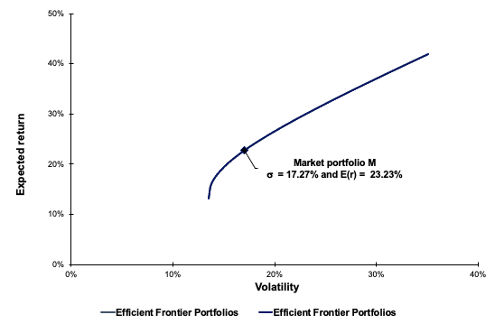
How to compute the IRR in Excel

November 13, 2021 by Jérémy PAULEN

How to compute the IRR in Excel

Jeremy PAULEN

In this article, Jérémy PAULEN (ESSEC Business School, Global Bachelor of Business Administration, 2019-2023) explains everything about the IRR function in Excel, which is used to compute the internal rate of return of a series of cash flow to evaluate the financial performance of an investment in relative terms.

What is the IRR?

The IRR represents the internal rate of return of an investment. It is closely related to the net present value (NPV) of the investment as the IRR is the discount rate that makes the NPV equal to zero.

Consider an investment represented by a series of cash flows CF₀, CF₁, CF₂, …, CF_T, which take into account the revenues and expenses of the project computed or forecasted at time 0 leading to capital inflows and outflows for the firm. The NPV of this investment is given by:

where r is the discount rate that takes into account the risk of the project.

The IRR corresponds to the value of the discount rate for which the NPV is equal to 0:

The IRR is the solution of a non-linear equation:

Note that this equation may have one solution, several solutions or no solution according to the sequence of cash flows.

The internal rate of return (IRR) is an important indicator in the decision-making process as it measures the financial performance of a project. The IRR is a relative measure as its unit is a percentage. The NPV is an absolute measure as its unit is the euro, the dollar, etc.

It makes it possible to measure the future financial performance of a project or a company. The higher the IRR is, the more interesting it is to launch the project.

The IRR can therefore be used in the case of a choice to be made between different investment perspectives, but also to evaluate the company’s share buyback programs.

A limit of using the IRR method is that it does not consider the size of a project. Cash flows are simply compared to the amount of capital outlay generating those cash flows. In other words, considering two projects A and B, the IRR of A may be lower than the IRR of B, while the NPV of A may be higher than the NPV of B.

The IRR function in Excel

How to use the IRR function in Excel?

In Excel, you can get the IRR function in the “Formulas” tab.
You can also type “= IRR (value, [guess])” in the cell where you want to compute the IRR.

The IRR function uses the following arguments:

Values: The cash flow series. Cash flows include investment values and net income.
Guess: a number guessed by the user that is close to the expected internal rate of return

Example

Example: consider a new factory modeled by the following series of cash flows:

CF₀ = -$50,000 (initial cost)
CF₁ = +$5,000 (net cash flow in year 1)
CF₂ = +$8,000 (net cash flow in year 2)
CF₃ = +$13,500 (net cash flow in year 3)
CF₄ = +$18,800 (net cash flow in year 4)
CF₅ = +$20,500 (net cash flow in year 5)

Excel file to compute the IRR of a series of cash flows

You can download below a short video which illustrates how to compute the IRR of a series of cash flows with Excel.

Useful resources

Microsoft IRR function

About the author

The article was written in November 2021 by Jérémy PAULEN (ESSEC Business School, Global Bachelor of Business Administration, 2019-2023)

My Marketing Developer Experience

November 13, 2021 by Jérémy PAULEN

My Marketing Developer Experience

In this article, Jérémy PAULEN (ESSEC Business School, Global Bachelor of Business Administration, 2019-2023) shares his experience as a marketing developer at the Tennis Club of Rosheim.

Tennis Club of Rosheim

Tennis Club of Rosheim was founded in 1970 and is owned by David Livernais. The premises are located in the sports center of Rosheim, in Alsace. The Tennis Club had 191 members in 2021 and several partners. The Club therefore organizes many events every year.

The club wishes to create a relationship of trust with its members as well as a friendly atmosphere.

My internship at the Tennis Club of Rosheim

During my studies at ESSEC Business School, I had the opportunity to undertake an internship as a marketing developer at the Tennis Club of Rosheim.

Source: Tennis Club Rosheim

I was involved with the marketing department, which is in charge of promoting the club to potential new members. The promotion of a business takes place in several stages. First of all, through the development of a visual identity. The visual identity or graphic identity is a set of coherent visual elements which make it possible to identify the same entity through the different communication media that it uses. Example: Coca-Cola and the color red are almost synonymous with each other. The company uses its signature color on all of its products and all of its marketing materials.

Given my experience in the visual field and my different skills, I was given the responsibility of developing a new visual identity. The only restriction I had was to use the orange color.

I first had to create a logo. The logo is the pillar of a company’s image. A professional logo allows a company to stand out from its competitors, to convey its values and to tell a story. It therefore needs to be studied. The logo I created is made up of three elements:

A tennis ball in the center of the image to evoke the main activity of the club
The date the club was founded: 1970. Integrating a date reassures potential customers Because it implies professional knowledge and experience acquired over the years.
And last but not the least: the name of the club.

Source: Tennis Club Rosheim

I wanted a simple and uncluttered logo to reach as many people as possible.

I also had to create multiple posters to announce the different events. Each of my creations had a similar color code: orange, green and yellow. Orange is the color of cheerfulness, generosity, ambition, and abundance, but more importantly the color of the company. Green symbolizes hope and nature. Yellow is associated with joy, good humor, and radiance.

Promotion also passes through word, including emails or flyers. On several occasions I had to communicate by email with members and partners. Communicating through this media involves many codes. We must respect the codes of politeness and avoid any awkwardness. The emails are written and thus visible at all times.

Every day, the club president organized a general meeting where he talked about global debriefing. The various meetings make it possible to clarify the week’s objectives and to distribute the tasks to the workforce. They also present an opportunity to give feedback and to integrate each employee in the decision-making process. For my part, I took this opportunity to propose a new method of communication: Tiktok.

During my time at the TC Rosheim, I also had the opportunity to organize a large-scale event. Many competitors meet each year for a big competition. It was therefore necessary to find sponsors to finance this event, in our case the main partner was KARANTA. I also had to find volunteers to supervise the event and ensure it was smoothly run.

My key learning outcomes

During my internship at the Tennis Club of Rosheim, I had the opportunity to develop the following (soft) skills:

To manage a team
To meet deadlines
To improve communication skills
To understand the needs and to listen to the expectations of (internal) clients
The ability to learn and to improve my different skills

Three key terms

I develop below three key terms to understand my work.

Visual identity

The visual identity or graphic identity is a set of coherent visual elements which make it possible to identify the same entity through the different communication media that it uses.

A participatory leader

The participatory leader likes to study all the proposals before making a decision. He or she encourages his or her employees and values their work and achievements. A key element is feedback.

Feedback

Feedback is a step back, a testimony on an event that occurred. It allows time to check if the meaning of a message is understood, determine if help is required and verify if everybody is involved.

Useful resources

Tennis Club Rosheim

About the author

The article was written in November 2021 by Jérémy PAULEN (ESSEC Business School, Global Bachelor of Business Administration, 2019-2023).

Portfolio Theory and Risk

Mathematical foundations

Effect of diversification on portfolio risk

Academic research

Why should I be interested in this post?

Related posts on the SimTrade blog

Useful resources

Academic research

About the author

Introduction

Modelling of portfolios

Portfolio weights

Portfolio return: the case of two assets

Portfolio return: the case of N assets

Basic principles on portfolio construction

Diversify

Portfolio Asset Allocation

Portfolio Rebalancing

Reduce investment costs as much as possible

Invest on a regular basis

Buying in the future

Types of portfolio

Aggressive Portfolio

Defensive Portfolio

Income Portfolio

Speculative Portfolio

Hybrid Portfolio

Socially Responsible Portfolio

Why should I be interested in this post?

Related posts on the SimTrade blog

Useful resources

Academic research

Business analysis

About the author

Introduction

Mathematical foundation of Black-Litterman model

Black-Litterman asset allocation in practice

Why should I be interested in this post?

Related posts on the SimTrade blog

Useful resources

Academic research

About the author

Review of academic literature on passive investing

Core principles of passive investing

Passive investing and Efficient Market Hypothesis

Estimation of the S&P500 return

Why should I be interested in this post?

Related posts on the SimTrade blog

Useful resources

Academic research

Business analysis

About the author

Introduction

Mathematical derivation of Beta

Use of beta

Excel file to compute the beta

Interpretation of the beta

Why should I be interested in this post?

Related posts on the SimTrade blog

Useful resources

Academic research

Business analysis

About the author

Introduction

Academic Literature

Mathematical derivation of Jensen’s alpha

Why should I be interested in this post?

Related posts on the SimTrade blog

Useful resources

Academic research

Business analysis

About the author

Security Market Line

Mathematical foundation

Beta and the market factor

Estimation of the Security Market Line

Why should I be interested in this post?

Related posts on the SimTrade blog

Useful resources

Academic research