In this article, Youssef Louraoui (Bayes Business School, MSc. Energy, Trade & Finance, 2021-2022) presents the Fama-MacBeth two-step regression method used to test asset pricing models.

This article is structured as follow: we introduce the Fama-MacBeth testing method. Then, we present the mathematical foundation that underpins their approach. We conclude with a practical case study followed by a discussion on econometric issues.

Introduction

Risk factors are frequently employed to explain asset returns in asset pricing theories. These risk factors may be macroeconomic (such as consumer inflation or unemployment) or microeconomic (such as firm size or various accounting and financial metrics of the firms). The Fama-MacBeth two-step regression approach a practical way for measuring how correctly these risk factors explain asset or portfolio returns. The aim of the model is to determine the risk premium associated with the exposure to these risk factors.

The first step is to regress the return of every asset against one or more risk factors using a time-series approach. We obtain the return exposure to each factor called the “betas” or the “factor exposures” or the “factor loadings”.

The second step is to regress the returns of all assets against the asset betas obtained in Step 1 using a cross-section approach. We obtain the risk premium for each factor. Then, Fama and MacBeth assess the expected premium over time for a unit exposure to each risk factor by averaging these coefficients once for each element.

Mathematical foundations

We describe below the mathematical foundations for the Fama-MacBeth two-step regression method.

Step 1: time-series analysis of returns

The model considers the following inputs:

• The return of N assets denoted by R_i for asset i observed over the time period [0, T].
• The risk factors denoted by F₁ for the market factor influencing the asset returns.

For each asset i from 1 to N, we estimate the following parameters:

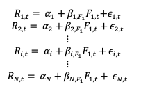
From this model, we obtain a series of coefficients: α_i which is the risk premium for asset i and the β_{i, F1 associated to the market risk factor.}

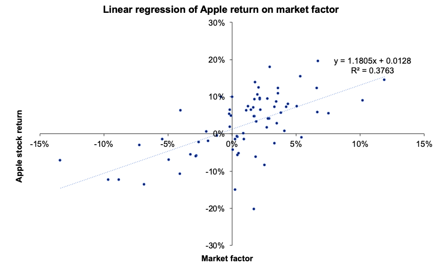
Figure 1 represents for a given asset the regression of a return with respect to the market factor (as in the CAPM). The slope of the regression line corresponds to the market beta of the regression.

Figure 1 Time-series regression.
Source : computation by the author.

The econometric issues (estimation bias, heteroscedasticity, and autocorrelation) related to the model are discussed in more details in the econometric limitation section.

Step 2: cross-sectional analysis of returns

For each period t from 1 to T, we estimate the following linear regression model:

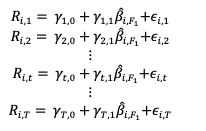
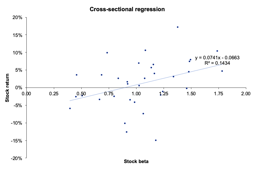
Figure 2 plots for a given period the cross-sectional returns and betas for a given point in time.

Figure 2 represents for a given period the regression of the return of all individual assets with respect to their estimated individual market beta.

Figure 2. Cross-sectional regression.
Source: computation by the author.

We average the gamma obtained for each data point. This is the way the Fama-MacBeth method is used to test asset pricing models.

Empirical study by Fama and MacBeth (1973)

Fama-MacBeth performed a second time the cross-sectional regression of monthly stock returns on the equity betas computed on the initial workings to account for the dynamic nature of stock returns, which help to compute a robust standard error to gauge the level of error and assess if there is any heteroscedasticity in the regression. The conclusion of the seminal paper suggests that the beta is “dead”, in the sense that it cannot explain returns on its own (Fama and MacBeth, 1973).

New empirical study

We downloaded a sample of end-of-month stock prices of large firms in the US economy over the period from March 31, 2016, to March 31, 2022. We computed monthly returns. To represent the market, we chose the S&P500 index.

We then applied the Fama-MacBeth two-step regression method to test the market factor (CAPM).

Figure 3 depicts the computation of average returns and the betas and stock in the analysis.

Figure 3. Computation of average returns and betas of the stocks.
Source: computation by the author.

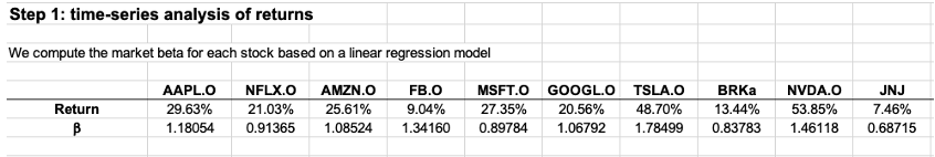
Figure 4 represents the first step of the Fama-MacBeth regression. We regress the average returns for each stock with their respective betas.

Figure 4. Step 1 of the regression: Time-series analysis of returns
Source: computation by the author.

The initial regression is statistically evaluated. To describe the behaviour of the regression, we employ a t-statistic. Since the p-value is in the rejection area (less than the significance limit of 5 percent), we can deduce that the market factor can at first explain the returns of an investor. However, as we are going deal in the later in the article, when we account for a second regression as formulated by Fama and MacBeth, the market factor is not capable of explaining on its own the return of asset returns.

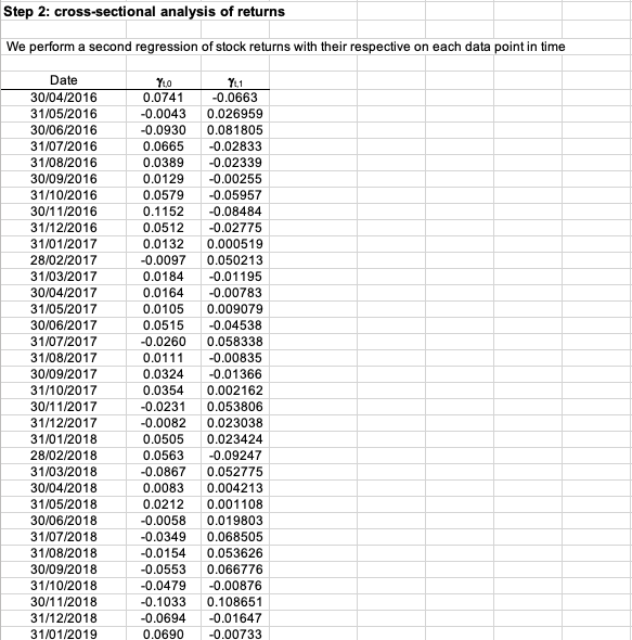
Figure 5 represents Step 2 of the Fama-MacBeth regression, where we perform for a given data point a regression of all individual stock returns with their respective estimated market beta.

Figure 5. Step 2: cross-sectional analysis of return.
Source : computation by the author.

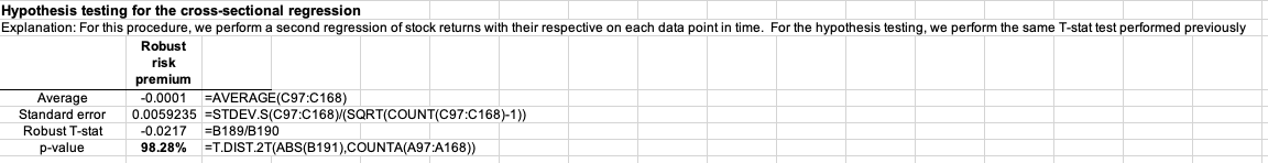
Figure 6 represents the hypothesis testing for the cross-sectional regression. From the results obtained, we can clearly see that the p-value is not in the rejection area (at a 5% significance level), hence we cannot reject the null hypothesis. This means that the market factor fails to explain properly the behaviour of asset returns, which undermines the validity of the CAPM framework. These results are in line with the Fama-MacBeth paper (1973).

Figure 6. Hypothesis testing of the cross-sectional regression.
Source: computation by the author.

Excel file for the Fama-MacBeth two-step regression method

You can find below the Excel spreadsheet that complements the explanations covered in this article to apply the Fama-MacBeth two-step regression method.

Econometric issues

Errors in data measurement

Because regression uses a sample instead of the entire population, a certain margin of error must be accounted for since the authors derive estimated betas for the sample.

Asset return heteroscedasticity

In econometrics, heteroscedasticity is an important concern since it results in unequal residual variance. This indicates that a time series exhibiting some heteroscedasticity has a non-constant variance, which renders forecasting ineffective because the time series will not revert to its long-run mean.

Asset return autocorrelation

Standard errors in Fama-MacBeth regressions are solely corrected for cross-sectional correlation. This method does not fix the standard errors for time-series autocorrelation. This is typically not a concern for stock trading, as daily and weekly holding periods have modest time-series autocorrelation, whereas autocorrelation is larger over long horizons. This suggests that Fama-MacBeth regression may not be applicable in many corporate finance contexts where project holding durations are typically lengthy.

Limitation of CAPM

Roll: selection of the appropriate market index

For the CAPM to be valid, we need to determine if the market portfolio is in the Markowitz efficient curve. According to Roll (1977), the market portfolio is not observable because it cannot capture all the asset classes (human capital, art, and real estate among others). He then believes that the returns cannot be captured effectively and hence makes the market portfolio, not a reliable factor in determining its efficiency.

Furthermore, the coefficients are sensitive to the market index chosen for the study. These shortcomings must be taken into account when assessing other CAPM studies.

Fama-MacBeth: Stability of the coefficients

The stability of the beta across time is difficult. Fama-MacBeth attempted to address this shortcoming by implementing its innovative approach. However, some points need to be addressed:

When betas are computed using a monthly time series, the statistical noise of the time series is considerably reduced as opposed to shorter time frames (i.e., daily observation).

Constructing portfolio betas makes the coefficient much more stable than when assessing individual betas. This is due to the diversification effect that a portfolio can achieve, reducing considerably the amount of specific risk.

Why should I be interested in this post?

Fama-MacBeth made a significant contribution to the field of econometrics. Their findings cleared the way for asset pricing theory to gain traction in academic literature. The Capital Asset Pricing Model (CAPM) is far too simplistic for a real-world scenario since the market factor is not the only source that drives returns; asset return is generated from a range of factors, each of which influences the overall return. This framework helps in capturing other sources of return.

Related posts on the SimTrade blog

▶ Jayati WALIA Capital Asset Pricing Model (CAPM)

▶ Youssef LOURAOUI Security Market Line (SML)

▶ Youssef LOURAOUI Origin of factor investing

▶ Youssef LOURAOUI Factor Investing

Useful resources

Academic research

Brooks, C., 2019. Introductory Econometrics for Finance (4th ed.). Cambridge: Cambridge University Press. doi:10.1017/9781108524872

Fama, E. F., MacBeth, J. D., 1973. Risk, Return, and Equilibrium: Empirical Tests. Journal of Political Economy, 81(3), 607–636.

Roll R., 1977. A critique of the Asset Pricing Theory’s test, Part I: On Past and Potential Testability of the Theory. Journal of Financial Economics, 1, 129-176.

American Finance Association & Journal of Finance (2008) Masters of Finance: Eugene Fama (YouTube video)

Business Analysis

NEDL. 2022. Fama-MacBeth regression explained: calculating risk premia (Excel). [online] Available at: [Accessed 29 May 2022].

About the author

The article was written in May 2022 by Youssef LOURAOUI (Bayes Business School, MSc. Energy, Trade & Finance, 2021-2022).

References

Academic research articles
Broadie, M., Glasserman P., Kou S. (1997) A Continuity Correction for Discrete Barrier Option. Mathematical Finance, 7:325-349.
Merton, R. (1973) Theory of Rational Option Pricing. The Bell Journal of Economics and Management Science, 4:141-183.
Paixao, T. (2012) A Guide to Structured Products – Reverse Convertible on S&P500
Reiner, E.S., Rubinstein, M. (1991) Breaking down the barriers. Risk Magazine, 4(8), 28–35.
Rich, D. R. (1994) The Mathematical Foundations of Barrier Option-Pricing Theory. Advances in Futures and Options Research: A Research Annual, 7:267-311.
Wang, B., Wang, L. (2011) Pricing Barrier Options using Monte Carlo Methods, Working paper.
Books
Haug, E. (1997) The Complete Guide to Option Pricing. London/New York: McGraw-Hill.
Hull, J. (2006) Options, Futures, and Other Derivatives. Upper Saddle River, N.J: Pearson/Prentice Hall.