In this article, Youssef LOURAOUI (Bayes Business School, MSc. Energy, Trade & Finance, 2021-2022) explains the specific risk of financial assets, a key concept in asset pricing models and asset management in practice.
This article is structured as follows: we start with a reminder of portfolio theory and the central concept of risk in financial markets. We then introduce the concept of specific risk of an individual asset and especially its sources. We then detail the mathematical foundation of risk. We finish with an insight of the relationship between diversification and risk reduction with a practical example to test this concept.
Portfolio Theory and Risk
Markowitz (1952) and Sharpe (1964) created a framework for risk analysis based on their seminal contributions to portfolio theory and capital market theory. All rational profit-maximizing investors attempt to accumulate a diversified portfolio of risky assets and borrow or lend to achieve a risk level consistent with their risk preferences given a set of assumptions. They established that the key risk indicator for an individual asset in these circumstances is its correlation with the market portfolio (the beta).
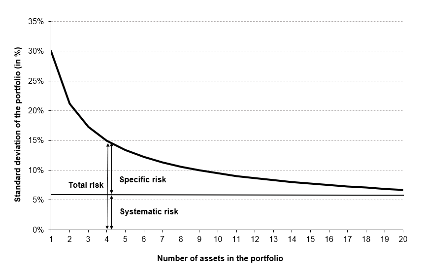
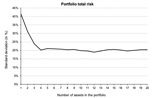
The variance of returns of an individual asset can be decomposed as the sum of systematic risk and specific risk. Systematic risk refers to the proportion of the asset return variance that can be attributed to the variability of the whole market. Specific risk refers to the proportion of the asset return variance that is unconnected to the market and reflects the unique nature of the asset. Specific risk is often regarded as insignificant or irrelevant because it can be eliminated in a well-diversified portfolio.
Sources of specific risk
Specific risk can find its origin in business risk (in the assets side of the balance sheet) and financial risk (in the liabilities side of the balance sheet):
Business risk
Internal or external issues might jeopardize a business. Internal risk is directly proportional to a business’s operational efficiency. An internal risk would include management neglecting to patent a new product, so eroding the company’s competitive advantage.
Financial risk
This pertains to the capital structure of a business. To continue growing and meeting financial obligations, a business must maintain an ideal debt-to-equity ratio.
Mathematical foundations
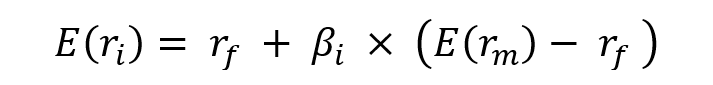
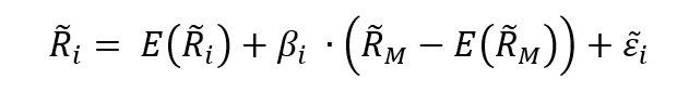
Following the Capital Asset Pricing Model (CAPM), the return on asset i, denoted by Ri can be decomposed as
Where:
- Ri the return of asset i
- E(Ri) the risk premium of asset i
- βi the measure of the risk of asset i
- RM the return of the market
- E(RM) the risk premium of the market
- RM – E(RM) the market factor
- εi represent the specific part of the return of asset i
The three components of the decomposition are the expected return, the market factor and an idiosyncratic component related to asset only. As the expected return is known over the period, there are only two sources of risk: systematic risk (related to the market factor) and specific risk (related to the idiosyncratic component).
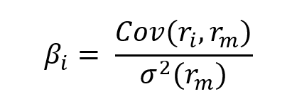
The beta of the asset with the market is computed as:
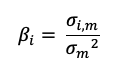
Where:
- σi,m : the covariance of the asset return with the market return
- σm2 : the variance of market return
The total risk of the asset measured by the variance of asset returns can be computed as:
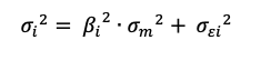
Where:
- βi2 * σm2 = systematic risk
- σεi2 = specific risk
In this decomposition of the total variance, the first component corresponds to the systematic risk and the second component to the specific risk.
Decomposition of returns
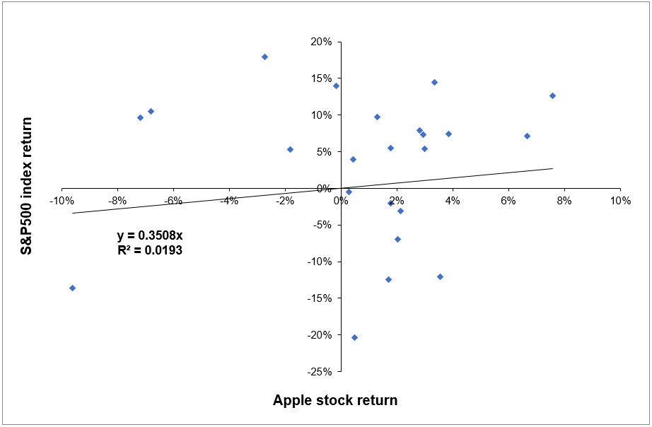
We analyze the decomposition of returns on Apple stocks. Figure 1 gives for every month of 2021 the decomposition of Apple stock returns into three parts: expected return, market factor (systematic return) and an idiosyncratic component (specific return). We used historical price downloaded from the Bloomberg terminal for the period 1999-2022.
Figure 1. Decomposition of Apple stock returns:
expected return, systematic return and specific return.
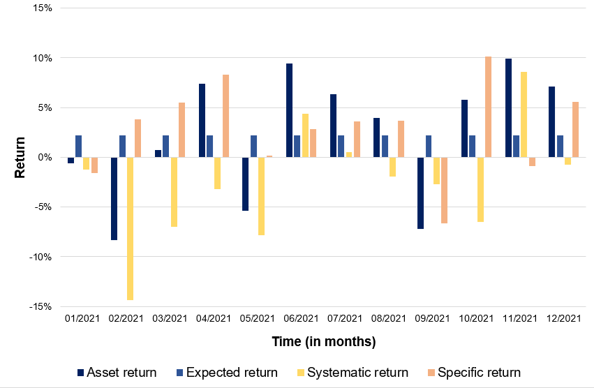 Computation by the author (data: Bloomberg).
You can download below the Excel file which illustrates the decomposition of returns on Apple stocks.

Why should I be interested in this post?
Investors will be less influenced by single incidents if they possess a range of firm stocks across several industries, as well as other types of assets in a number of asset classes, such as bonds and stocks.
An investor who only bought telecommunication equities, for example, would be exposed to a high amount of unsystematic risk (also known as idiosyncratic risk). A concentrated portfolio can have an impact on its performance. This investor would spread out telecommunication-specific risks by adding uncorrelated positions to their portfolio, such as firms outside of the telecommunication market.
Related posts on the SimTrade blog
▶ Louraoui Y. Systematic risk and specific risk
▶ Louraoui Y. Systematic risk
▶ Louraoui Y. Beta
▶ Louraoui Y. Portfolio
▶ Louraoui Y. Markowitz Modern Portfolio Theory
▶ Walia J. Capital Asset Pricing Model (CAPM)
Useful resources
Academic research
Evans, J.L., Archer, S.H. 1968. Diversification and the Reduction of Dispersion: An Empirical Analysis. The Journal of Finance, 23(5): 761–767.
Markowitz, H. 1952. Portfolio Selection. The Journal of Finance, 7(1): 77-91.
Mossin, J. 1966. Equilibrium in a Capital Asset Market. Econometrica, 34(4): 768-783.
Sharpe, W.F. 1963. A Simplified Model for Portfolio Analysis. Management Science, 9(2): 277-293.
Sharpe, W.F. 1964. Capital Asset Prices: A Theory of Market Equilibrium under Conditions of Risk. The Journal of Finance, 19(3): 425-442.
Tole T.M. 1982. You can’t diversify without diversifying. The Journal of Portfolio Management. Jan 1982, 8 (2) 5-11.
About the author
The article was written in April 2022 by Youssef LOURAOUI (Bayes Business School, MSc. Energy, Trade & Finance, 2021-2022).

 Source: Computations from the author.
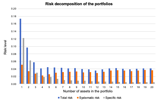 Source: Computations from the author.
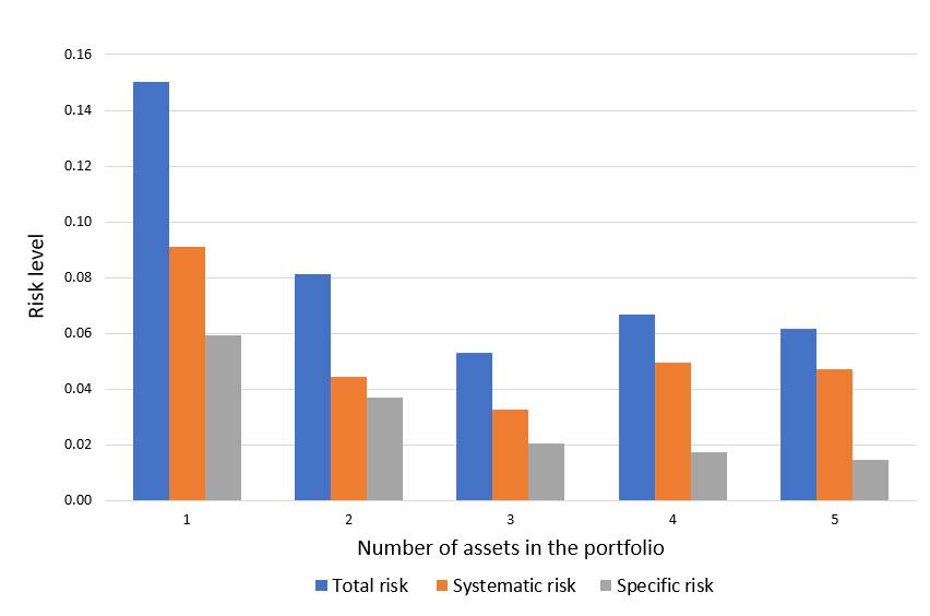 Source: Computation from the author.
 Source: Computation from the author.