Implied Volatility Surface: Smiles, Smirks and Term Structure

June 29, 2026 by Saral BINDAL

In this article, Saral BINDAL (Indian Institute of Technology Kharagpur, Metallurgical and Materials Engineering, 2024-2028 & Research assistant at ESSEC Business School) explains the implied volatility surface: its characteristic shapes, static arbitrage constraints, and application using S&P 500 index options data.

Introduction

In financial markets characterized by uncertainty, volatility is a crucial factor in the valuation of derivative securities. For options traders, an option price is essentially volatility. Although options are traded at monetary prices, professionals routinely quote and compare them in terms of implied volatility (%), making volatility the common language of options markets. Moreover, in a reverse way, implied volatility occupies a central role as a forward-looking indicator that reflects the market’s expectations of future price fluctuations embedded in option prices.

Under the Black-Scholes-Merton (BSM) model, volatility is assumed to be constant and independent of option characteristics like the strike price (K) and the time to maturity (T). Empirical evidence, however, reveals that implied volatility varies across option contracts and especially depends on both parameters K and T of the option.

Implied volatility curves: the strike dimension

Volatility curves represent a cross-sectional view of the implied volatility surface (IVS), depicting the relationship between implied volatility and strike price for a fixed maturity. They are constructed by plotting implied volatility as a function of strike while holding time-to-maturity constant.

The volatility curves are commonly observed in two distinct shapes, most notably the volatility smile and the volatility smirk. A detailed discussion of the empirical relationship between implied volatility and option moneyness, the associated stylized facts, and their economic interpretation can be found in the article Volatility curves: smiles and smirks.

Figure 1 below illustrates the implied volatility smile (1a) and smirk (1b).

Figure 1a and 1b. Implied Volatility Smile and Smirk
Implied Volatility Curves (smile and smirk)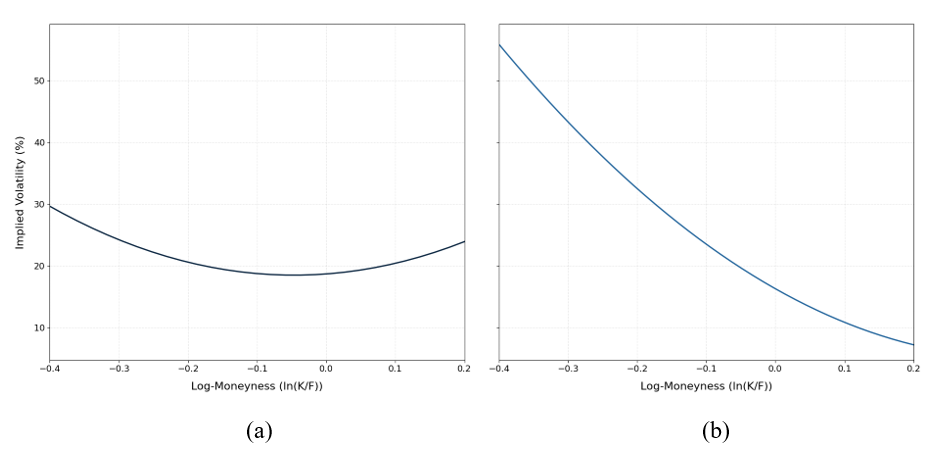
Source: computation by the author (with python).

Term structure of implied volatility: the maturity dimension

While volatility curves describe the strike dependence of implied volatility, the maturity dimension captures how implied volatility varies across expiration dates for a given strike. This relationship is commonly referred to as the term structure of implied volatility.

Using daily implied volatility data for S&P 100 index options (December 1983 to September 1987), Stein (1989) documented that volatility shocks are transmitted across maturities more strongly than predicted by standard rational expectations theory. Under this standard theoretical framework, because implied volatility is strongly mean-reverting, a near-term shock should naturally decay over time, causing long-dated implied volatilities to change by only a fractional amount. However, following an increase in short-dated implied volatility, long-dated implied volatilities tend to rise by a disproportionately large amount, indicating that changes in near-term uncertainty heavily influence market expectations over a broad range of maturities.

Using data for options on the S&P 500, FTSE 100, DAX 30, CAC 40, and Nikkei 225 stock indexes spanning the period May 9, 1994 to October 12, 2001, Mixon (2007) suggested mean reversion as a key characteristic of the implied volatility term structure. While short-dated implied volatilities exhibit substantial sensitivity to changes in market conditions, long-dated implied volatilities remain comparatively stable, reflecting expectations of convergence toward a long-run volatility level. Consequently, the term structure is generally upward sloping (contango) during periods of low market uncertainty but may become inverted (backwardation) during episodes of market stress, when short-term volatility rises sharply.

Figure 2 illustrates an upward-sloping (2a) and a downward-sloping (2b) implied volatility term structure.

Figure 2a and 2b. Implied Volatility Term Structure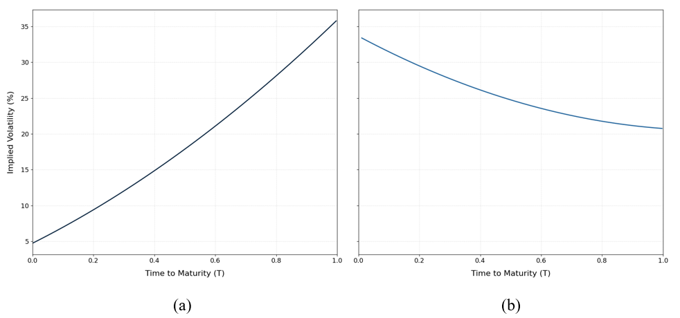

Source: computation by the author (with python).

Christoffersen, Heston, and Jacobs (2009) demonstrate that the volatility term structure is not necessarily monotonic, arguing that capturing its true dynamics requires multifactor stochastic volatility frameworks. Evaluating European S&P 500 call options from 1990 through 2004, their empirical evidence reveals that implied volatility frequently displays significant curvature across maturities. This non-monotonic curvature is difficult to reconcile with traditional single-factor specifications like the benchmark Heston (1993) model, which restricts the term structure of implied volatility because it relies on only a single variance factor to model volatility over time.

Volatility Surface

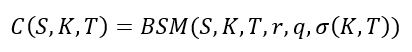
The volatility surface provides a three-dimensional representation of implied volatility across strike prices and maturities. It is represented by the function σ(K,T), which assigns an implied volatility to each combination of strike price K and time to maturity T that reproduces the observed market option prices under the Black-Scholes-Merton (BSM) model.

Call option price formula under the BSM

Constructed from a cross-section of traded options, the volatility surface provides a comprehensive description of how the market prices uncertainty across both strike price (K) and maturity (T).

Arbitrage constraints

In practice, market option quotes are available only for a discrete set of strikes and maturities. Constructing a continuous volatility surface therefore requires interpolation and smoothing techniques. To ensure economic consistency, we must have σ(K,T) ≥ 0 for all strikes K and expirations T and the resulting surface must satisfy the static no-arbitrage conditions: namely the absence of butterfly arbitrage across strikes and calendar-spread arbitrage across maturities. (see, Breeden & Litzenberger, 1978; Gatheral, 2006)

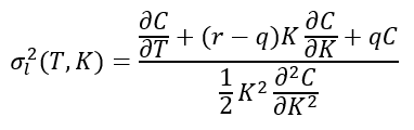
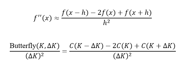
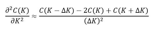
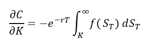
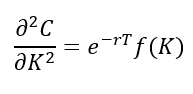
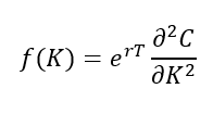
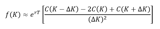
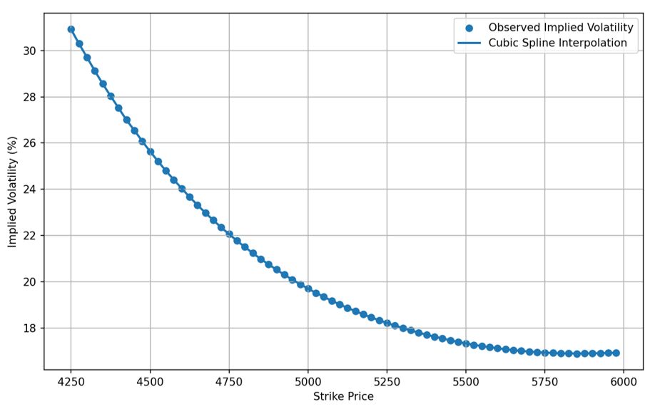
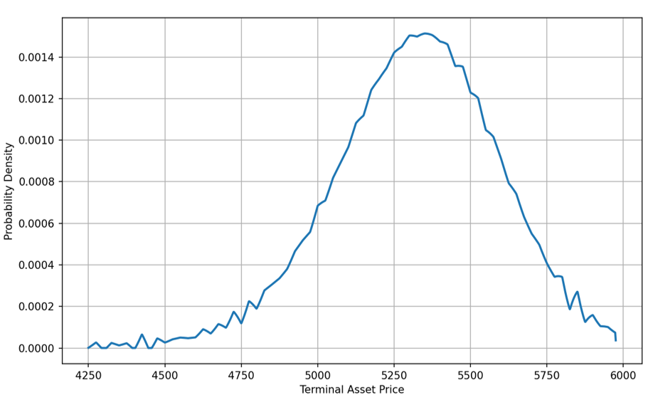
The absence of butterfly arbitrage requires option prices to remain convex with respect to strike. Equivalently, the risk-neutral probability density implied by option prices must remain non-negative across all strikes, this condition can be expressed as:

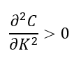
Conditon for the absence of butterfly arbitrage

A violation of this condition implies a negative risk-neutral probability density over some range of strikes and leads to arbitrage opportunities.

The absence of calendar-spread arbitrage states that with increase in maturity of an option, it should not result in a reduction of its value, since a longer-dated option provides all the rights of an otherwise identical shorter-dated option together with additional time for favourable price movements to occur. In volatility surface modelling, this condition is typically expressed in terms of the total implied variance

Total implied variance formula

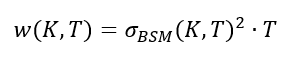
where σ_BS(K,T) denotes the Black-Scholes-Merton implied volatility for strike K and maturity T. Total implied variance measures the total accumulated expected variance over the entire life of the option

For a fixed strike, total implied variance must be non-decreasing with maturity

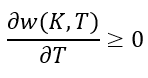
Conditon for the absence of calendar-spread arbitrage

A violation would imply that a longer-dated option embeds less cumulative uncertainty than a shorter-dated option at the same strike, resulting in an arbitrage opportunity.

Together, the butterfly-arbitrage and calendar-spread-arbitrage constraints ensure that the interpolated volatility surface produces arbitrage-free option prices and a valid risk-neutral distribution.

An Empirical Analysis of the S&P 500 Implied Volatility Surface

In this section, we discuss how an implied volatility surface can be estimated from the S&P 500 index observed market option prices using a parametric model to fit the data and how the parameters can be adjusted to represent different macro-economic stress conditions.

Data collection and filtration

To construct the implied volatility surface, we import the S&P 500 index option chain (set of call and put options across various strikes and maturities) directly from Yahoo! Finance. Because raw market data often contains stale quotes and asynchronous prices, we apply a robust set of filtering techniques to clean the dataset before model estimation.

First, we apply illiquidity filters, removing any option contracts with zero trading volume or zero open interest. Second, we filter the dataset to retain only Out-of-the-Money (OTM) options (OTM puts where K < S₀, and OTM calls where K > S₀). This is a standard practice, as implied volatility is theoretically independent of option type due to Put-Call Parity, focusing strictly on OTM contracts ensures we utilize the most liquid instruments (liquidity being measured by the bid-ask spread) to minimize pricing noise.

Third, we enforce intrinsic value and no-arbitrage boundary conditions. Any contracts with mispriced or economically impossible quotes are filtered out by verifying the upper and lower price bounds for the option contracts as given below

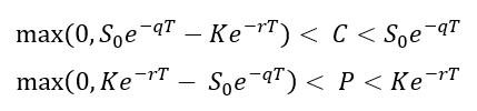
Call and Put option mid-price bounds

where:

K: strike price of the option
S₀: spot price of the underlying asset
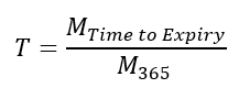
T: time to maturity
C: mid-price of a call option
P: mid-price of a put option
r: risk-free rate
q: continuous dividend yield

Finally, we check for vertical (strike) arbitrage to ensure the data adheres to fundamental shape restrictions. We sort the contracts by time-to-maturity and then by strike price in ascending order. We then verify shape monotonicity: for any given maturity, call prices must strictly decrease as the strike price increases, and put prices must strictly increase as the strike price increases. Applying these standard empirical filters ensures a clean, arbitrage-free dataset ready for surface estimation.

Methodology

To model and plot the implied volatility surface as shown below in Figure 1, we implement a parametric approach originally proposed by Dumas, Fleming, and Whaley (1998). This technique fits a deterministic volatility function (DVF) directly through the observed option market data. Under this framework, the implied volatility function is expressed as a second-order polynomial function across log-moneyness (M) and time-to-maturity (T):

DVF Formula

where:

α₀ : Measures the baseline implied volatility level where both log-moneyness and time-to-maturity are equal to zero. Geometrically, this shifts the entire surface straight up or down uniformly
α₁ : Measures the rate of change of volatility across different strikes. Geometrically, this rotates the surface along the moneyness axis, tilting the left wing (puts) up and the right wing (calls) down.
α₂ : Measures the rate of change of the curvature across strikes, defining how sharply the volatility curve bends. Geometrically, this bends the surface into a U-shaped bowl or flattens it into a smooth plane.
α₃ : Measures the rate of change of volatility across the horizon, establishing the slope of the term structure. Geometrically, this tilts the surface front-to-back, altering the premium difference between short-term and long-term contracts.
α₄ : Measures the rate of change of the curvature in the volatility in the term structure across different maturities. Geometrically, this creates a non-linear bend along the time horizon axis.
α₅ : Measures the co-dependency between moneyness and time-to-maturity, modelling how the skew changes as maturity extends. Geometrically, this causes the corners to bend upward or downward simultaneously.

In the polynomial function above, we utilize the log-forward moneyness (M), defined as:

Log-forward moneyness formula

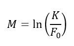
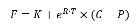
where F₀ is the forward price of the underlying asset, calculated as:

Forward price formula

This is usually done in practice because it is F₀, and not S₀, that represents the expected stock price on the option’s maturity date in a risk-neutral world. Consequently, traders often define an “at-the-money” option as a contract where K = F₀, rather than an option where K = S₀.

To fit this model, we first apply a numerical root-finding algorithm to invert the Black-Scholes-Merton (BSM) pricing model against observed market prices (mid prices defined as the average of bid and ask prices) to extract the market implied volatilities. We restrict our sample to contracts with maturities under one year (T < 1.0) and a log-moneyness of |M| < 0.45. This filters out deep Out-of-the-Money (OTM) options, which typically suffer from low trading volumes and wide bid-ask spreads, as they are primarily held for structural tail-hedging by institutional investors.

Finally, we apply Ordinary Least Squares (OLS) regression to the filtered dataset to solve for the six α parameters simultaneously. Once estimated, these parameters can be used to generate the implied volatility curves, term structures, and 3D surfaces under various macroeconomic stress scenarios, as discussed below.

Empirical Results

Figure 3 illustrates the estimated implied volatility surface of the S&P 500 index using options data collected on June 18, 2026. The market environment at the time of collection was defined by an index spot price (S₀) of $7496.04, a risk-free interest rate (r) of 3.658%, and a continuous dividend yield (q) of 1.04%. Based on these inputs, the resulting empirical surface is presented below.

Figure 3. Implied Volatility Surface of the S&P 500 index options (June 18, 2026)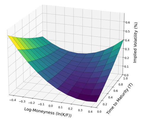

Source: computation by the author (with python).

From the surface, we can observe that amid ongoing US-Iran tensions in the Middle East, out-of-the-money (OTM) put options exhibit high implied volatility for short-term maturities. This reflects panic buying of downside protection due to fears of conflict escalation and immediate uncertainty in the market. Toward the far end of the maturity, however, the surface balances out with OTM call options. This indicates that while near-term sentiment is dominated by risk aversion, long-term market expectations are highly speculative, positioning for a potential recovery once the geopolitical uncertainty resolves. To isolate and observe these market dynamics more precisely, the individual implied volatility smiles (by strike) and term structures (by maturity) are plotted below.

Figure 4 illustrates the implied volatility curves for three distinct maturities. As discussed above, we can clearly observe the steep downside skew flattening out and transitioning into a asymmetric smile as maturity increases.

Figure 4. Implied Volatility Curves of the S&P 500 options (June 18, 2026)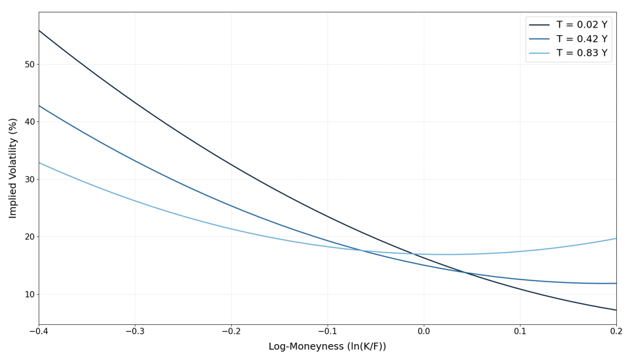

Source: computation by the author (with python).

Figure 5 illustrates the implied volatility term structure (up to 1 year) for three different strike prices. For out-of-the-money (OTM) call options, we can observe that the term structure is upward-sloping, indicating a long-term uncertainty alongside expectations of an upward market movement. Conversely, the OTM put option term structure is inverted and reflecting high short-term panic and uncertainty. Over the time horizon, this near-term panic subsides, balancing out with the OTM call options in the long run.

Figure 5. Implied Volatility Term Structure of the S&P 500 index options (June 18, 2026)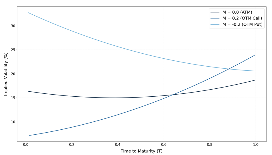

Source: computation by the author (with python).

The at-the-money (ATM) option term structure exhibits a shallow, non-monotonic U-shape, characterized by elevated short-dated volatility, a flattened middle region, and higher long-term volatility. This reflects that, in the short-to-medium term, the curve demonstrates the classic mean-reversion, where the immediate geopolitical shock dissipates and flattens out over a 3-to-6-month horizon. Conversely, the upward drift at the longer end of the mature horizon reflects the structural term premium demanded by investors to account for broader, open-ended macroeconomic uncertainties, as discussed above in the stylized facts section.

Structural Shifts under Macroeconomic Stress: A Comparative Scenario Analysis

Figure 6 provides a compelling visual framework for observing how the implied volatility surface structurally shifts under different stress conditions. The surface on the left (a) represents the systemic crash caused by the COVID-19 pandemic (2020), while the surface on the right (b) illustrates the hypothetical impact on index options if the ongoing US-Iran conflict were to escalate significantly. These surfaces are constructed by adjusting the values of the six model parameters estimated in the preceding section; as such, they serve as illustrative examples of structural shifts rather than exact numerical forecasts.

Figures 6a and 6b. Implied Volatility Surface of the S&P 500 options under different stress environments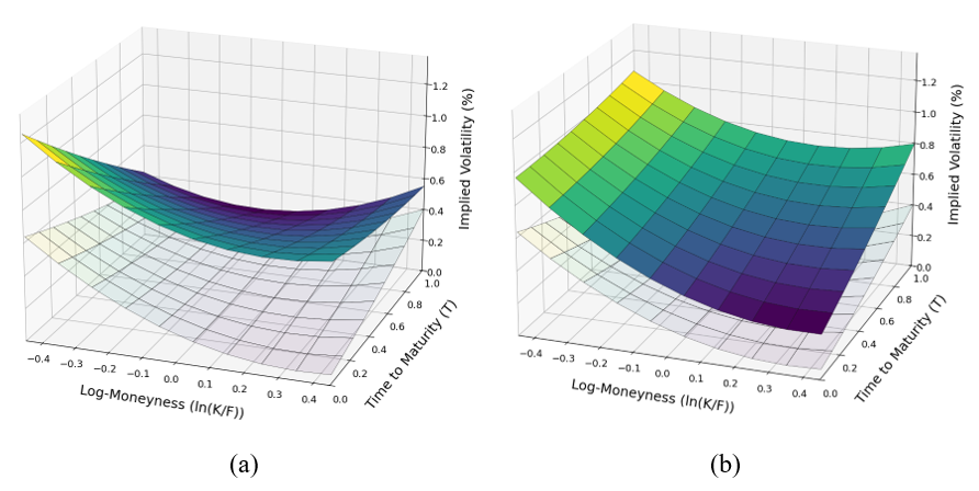

Source: computation by the author (with python).

Note: In both figures, the lightly shaded surface serves as the baseline, representing the actual market implied volatility surface as of June 18, 2026.

From Figure 6a, we can observe a massive surge in overall implied volatility across the board, driven by widespread panic buying of both out-of-the-money (OTM) puts and calls. This systemic shock resulted in a relatively flatter skew but severe inversion across the maturity spectrum, reflecting the acute, immediate fear of economic collapse as global lockdowns were implemented.

In contrast, Figure 6b models a scenario where the US-Iran conflict escalates into a full-scale regional crisis. Such an event would severely disrupt global oil supply chains, acting as a prolonged macroeconomic drag that hits S&P 500 corporate earnings over many months. Because this represents a lingering economic threat rather than an overnight liquidity freeze, the market’s response is highly asymmetric: demand is heavily concentrated in OTM puts for long-term downside protection and a steady increase in long-term implied volatility across the maturity.

While these stress scenarios represent extreme events, day-to-day movements follow structured patterns. Cont and Da Fonseca (2002) showed that daily dynamic deformations of the S&P 500 volatility surface are not chaotic. Instead, using principal component analysis, they demonstrated that surface movements are driven by just a few common statistical factors: parallel shifts, changes in the strike slope (skew), and twists in the maturity curvature.

You can download the Python code provided below, for the construction of the implied volatility curves, term structures and surfaces under different stress conditions as discussed above.

Alternatively, you can download the R code below with the same functionality as in the Python file.

Volatility Surface Models

A volatility surface determines the risk-neutral distributions implied by option prices (see Option Implied Risk-Neutral Distribution), but it does not uniquely specify the underlying stochastic process governing asset-prices. As highlighted by Cont (2006), this introduces significant model uncertainty: different mathematical frameworks can calibrate perfectly to the exact same market volatility surface today, yet yield wildly divergent prices and hedges for exotic options because they imply different future surface dynamics. Consequently, a substantial body of research has focused on developing models capable of reproducing both the observed shape of the volatility surface and its evolution through time.

The principal modelling approaches include local volatility models, stochastic volatility models, parametric surface models and, more recently, rough volatility models.

Local Volatility Models

In the standard BSM formula, volatility is assumed constant, which however does not correspond to reality, as markets exhibit volatility smile and skews. Local volatility model, extends the BSM, by assuming that volatility is a function of stock price (S_t) and time (t), and the instantaneous local volatility is given by σ_t( S_t,t).

The Dupire (1994) formula that links the instantaneous local volatilities, to the implied volatility surface is given as follows:

Local volatility formula

Stochastic Volatility Models

Stochastic volatility refers to the modelling of volatility using time-dependent stochastic processes, in contrast to the constant volatility assumption made in the standard BSM model. These models are better able to capture the observed features such as volatility clustering and mean reversion. One of the most widely used stochastic volatility models is the Heston (1993) model. The model describes the dynamics of the underlying asset price and its variance using a system of two coupled stochastic differential equations (SDEs), given by:

Stochastic volatility formula

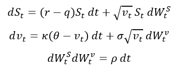
Where:

S_t: is the asset price
v_t: is the instantaneous variance
r: is the risk-free interest rate
q: is the continuous dividend yield
κ: is the speed of mean reversion
θ: is the long-run variance level
σ: is the volatility of variance (volatility-of-volatility)
ρ: is the correlation between shocks to the asset price and variance

Parametric Surface Models

Parametric volatility surface models are used to interpolate and extrapolate implied volatility across strikes and maturities, for sparse or illiquid strikes and ensure the resulting surface is free from static arbitrage (butterfly and calendar arbitrage).

Among the most widely used approaches is the SVI (Stochastic Volatility Inspired) parametrization, developed by Gatheral and Jacquier (2014), which is commonly applied to equity and index volatility surfaces. It models the total implied variance as a function of log-moneyness, providing a parsimonious representation of the volatility smile.

Other important parametric frameworks include the SABR model (Stochastic Alpha, Beta, Rho), which is widely used in interest rate and FX markets, and SSVI (Surface SVI), which extends the SVI framework to ensure arbitrage-free surface dynamics across maturities.

Rough Volatility Models

Rough volatility models represent one of the most important recent developments in volatility modelling. Gatheral, Jaisson, and Rosenbaum (2018) provided the empirical evidence that log-volatility behaves essentially as a fractional Brownian motion with Hurst exponent H of order 0.1, at any reasonable timescale.

The Hurst exponent (H) is a statistical parameter that characterises the roughness of a stochastic process: when H = 0.5, the process reduces to a standard Brownian motion with no memory, corresponding to a random walk. Whereas, values of H > 0.5 indicate persistent behaviour, while H < 0.5 imply anti-persistence, where increments tend to reverse direction more frequently, leading to rougher sample paths.

This observation, led to adoption of the fractional stochastic volatility (FSV) model of Comte and Renault (1998). The Rough FSV (RFSV) in contrast to FSV, is remarkably consistent with ﬁnancial time series data. Compared to classical stochastic volatility models, it better captures the extremely rough nature of volatility paths and enables improved forecasting of realized volatility.

Why should I be interested in this post?

Implied volatility surfaces are among the most important tools in modern quantitative finance. They play a central role in the pricing and hedging of derivatives, particularly exotic options, and are widely used in risk management, stress testing, and scenario analysis. A good understanding of volatility surfaces is therefore essential for students, practitioners, and anyone seeking a career in derivatives, quantitative finance, trading, or risk management.

Useful resources

Academic research on Option pricing

Black, F., & Scholes, M. (1973). The pricing of options and corporate liabilities. Journal of Political Economy, 81(3), 637-654.

Breeden, D. T., & Litzenberger, R. H. (1978). Prices of state-contingent claims implicit in option prices. Journal of Business, 51(4), 621-651.

Hull J.C. (2015) Options, Futures, and Other Derivatives, Eleventh Edition, Global Edition, Chapter 15 – The Black-Scholes-Merton model, 338-369.

Merton, R.C. (1973). Theory of rational option pricing. The Bell Journal of Economics and Management Science, 4(1), 141-183.

Academic Research on Stylized Facts on Option Volatility

Christoffersen, P., Heston, S., & Jacobs, K. (2009). The shape and term structure of the index option smirk: Why multifactor stochastic volatility models work so well. Management Science, 55(12), 1914-1932.

Heston, S. L. (1993). A closed-form solution for options with stochastic volatility with applications to bond and currency options. The Review of Financial Studies, 6(2), 327-343.

Mixon, S. (2007). The implied volatility term structure of stock index options. Journal of Empirical Finance, 14(3), 333-354.

Stein, J. C. (1989). Overreactions in the options market. Journal of Finance, 44(4), 1011-1023.

Academic Research on Empirical Analysis of Implied Volatility Surfaces

Cont, R., & Da Fonseca, J. (2002). Dynamics of implied volatility surfaces. Quantitative Finance, 2(1), 45-60.

Gatheral, J. (2006). The Volatility Surface: A Practitioner’s Guide. John Wiley & Sons, Chapter 2 – Implied Volatility Surface, 25-42.

Hull J.C. (2015) Options, Futures, and Other Derivatives, Eleventh Edition, Global Edition, Chapter 20 – Volatility smiles and volatility surfaces, 451-467.

Dumas, B., Fleming, J., and Whaley, R.E. (1998). Implied volatility functions: Empirical tests. The Journal of Finance, 53(6), 2059-2106.

Academic Research on Implied Volatility Surface Models

Comte, F., & Renault, E. (1998). Long memory in continuous-time stochastic volatility models. Mathematical Finance, 8(4), 291-323.

Cont, R. (2006). Model uncertainty and its impact on the pricing of derivative instruments. Mathematical Finance, 16(3), 519-547.

Dupire, B. (1994). Pricing with a smile. Risk, 7(1), 18-20.

Gatheral, J., & Jacquier, A. (2014). Arbitrage-free SVI volatility surfaces. Quantitative Finance, 14(1), 59-71.

Gatheral, J., Jaisson, T., & Rosenbaum, M. (2018). Volatility is rough. Quantitative Finance, 18(6), 933-949.

Heston, S. L. (1993). A closed-form solution for options with stochastic volatility with applications to bond and currency options. Review of Financial Studies, 6(2), 327-343.

About the author

The article was written in June 2026 by Saral BINDAL (Indian Institute of Technology Kharagpur, Metallurgical and Materials Engineering, 2024-2028 & Research assistant at ESSEC Business School). His interests include tracking geopolitical developments and analysing their direct impact on macroeconomic factors such as inflation, trade balances, and currency volatility, with a focus on using data to quantify these global economic ripple effects.

Discover all posts written by Saral BINDAL.

CBOE Volatility Index

June 28, 2026June 28, 2026 by Saral BINDAL

In this article, Saral BINDAL (Indian Institute of Technology Kharagpur, Metallurgical and Materials Engineering, 2024-2028 & Research assistant at ESSEC Business School) explains the CBOE methodology for the construction of the volatility index or ‘VIX’.

Introduction

The Chicago Board Options Exchange (CBOE) Volatility Index, or VIX, is a real-time market index designed to measure the market’s expectation of 30-day forward-looking annualized volatility. It is option-based, calculated using the market prices of S&P 500 index options to gauge expected volatility.

History

In 1993, CBOE Global Markets introduced the CBOE Volatility Index (VIX Index). Originally designed by Robert E. Whaley (1993) to measure the market’s expectation of 30-day volatility, the index was calculated using an option-pricing model to derive the implied volatility of at-the-money S&P 100 index (OEX Index) options. The VIX Index quickly became the premier benchmark for U.S. stock market volatility and is widely referred to as the market’s “fear gauge”.

Ten years later in 2003, CBOE partnered with Goldman Sachs to completely overhaul the index. This update introduced a methodology independent of option-pricing models, adapting the seminal theoretical framework for model-free implied variance established by Britten-Jones and Neuberger (2000) alongside the practical replication insights of Demeterfi et al. (1999). This modern version of the VIX shifted its underlying base to the broader S&P 500 index. Rather than tracking a narrow selection of options, it estimates market expectations by aggregating a heavily weighted cross-section of SPX puts and calls across a wide range of strike prices.

Academic research confirms that this model-free aggregation method captures more information and provides a more efficient forecast of future realized volatility than individual Black-Scholes implied volatilities (Jiang & Tian, 2005).

Market Behavior

While VIX is often regarded as the market’s fear index, it might give one a false impression that it moves opposite to the S&P 500. Mathematically it has no directional bias, and only measures the magnitude of expected volatility. Instead, the real-world inverse relationship is driven by corporate capital structures and asymmetric investor behavior. As Black (1976) pointed out, when a stock price drops, a company’s financial leverage automatically increases, making the equity riskier and naturally driving up volatility.

Furthermore, market sell-offs trigger a sudden panic where investors rush to buy portfolio insurance (put options) all at once. Because the supply of this insurance is limited, options market makers must aggressively raise prices to protect themselves. Gârleanu et al. (2009) formalize this mechanism, demonstrating that because market makers cannot perfectly hedge their positions, concentrated investor demand directly drives option pricing and inflates implied volatility premiums. Since the VIX is calculated directly from these option prices, this demand-pressure mechanically forces the index to spike.

This same demand explains why the S&P 500 and the VIX occasionally rise together. During massive market rallies, investors experience FOMO (Fear of Missing Out) and rush to buy upside call options, or quickly buy puts to lock in their rapid gains. Just like during a market crash, this sudden increase in demand for options overwhelms market makers. To protect themselves, they hike option prices, which mechanically forces the VIX up even as the stock market climbs.

Option Selection Procedure

Selecting Eligible Expiration Dates

The VIX is designed to measure the market’s expectation of volatility over the next 30 calendar days. However, listed S&P 500 options rarely expire exactly 30 days from the calculation date. To address this, the methodology selects two option maturities: a near-term maturity of less than 30 days and a next-term maturity of more than 30 days remaining. Variance estimates are calculated for both maturities and subsequently interpolated to obtain a constant 30-day measure of expected volatility.

In the CBOE volatility index calculation methodology, time to expiration of a constituent option series, is calculated by dividing the number of minutes until expiration (M_{Time to Expiry}) of the selected options (rounded down to the nearest minute) by the number of minutes in a year (M₃₆₅).

VIX Time to Expiration Formula

Estimating the Forward Index Level

The next step is to estimate the forward index level of the S&P 500 using option markets prices. It represents the market’s expectation of the index value at expiration under the risk-neutral measure and serves as the reference point for selecting the relevant option contracts used in the calculation.

It is calculated using the principle of put-call parity, specifically by finding the unique strike price where the price difference between the call and the put option is at its absolute minimum.

VIX Forward Price Formula

Where:

F: The forward index level
K: The smallest strike price at which the absolute difference between the call price and the put price is the smallest (|C – P| is minimized).
C: The market price (midpoint of the bid-ask spread) of the call option at the strike price K_min.
P: The market price (midpoint of the bid-ask spread) of the put option at the strike price K_min.
R: The risk-free interest rate (typically based on U.S. Treasury bills matching the option’s maturity).
T: The time to expiration (expressed as a fraction of a calendar year).

Determining K₀

Once the forward index level has been estimated, we then identify K₀, defined as the first strike price equal to or immediately below the forward index level (F). This strike acts as a reference point for the option selection process, separating the out-of-the-money put options from the out-of-the-money call options used in the calculation.

Selecting Out-of-the-Money Options

The VIX methodology uses a wide range of out-of-the-money (OTM) put and call options. OTM options are sensitive to changes in expected future volatility and provide information about the market’s expectations across a broad range of potential future outcomes. By incorporating both downside and upside option prices, the methodology captures the entire market-implied distribution of future index values rather than relying on a single option contract.

Variance Calculation

The Contribution of Individual Options Contracts

Each selected option contributes unique information about the market’s expectation of future variance. The weight of this contribution depends on three key factors: the option’s mid-price (Q(K_i)), the strike spacing (ΔK_i) between neighbouring contracts, and the inverse square of its strike price (1/^(K_i)2). This precise weighting scheme ensures that information from the entire out-of-the-money option chain is integrated into the final variance estimate.

VIX Option Contribution Formula

where for:

Strike Spacing Formula

The VIX Variance Formula

The option selection and weighting procedure described above is formally represented by the VIX variance formula. Rather than estimating volatility from a single option, the formula aggregates information from all selected option contracts to produce an estimate of expected future annualized variance.

VIX Variance Formula

Where:

σ²: Annualized variance
T: Time to expiration (in years)
F: Option-implied forward price
K_i: Strike price of the i^th out-of-the-money option
K₀: First strike equal to or otherwise immediately below the forward index level, F
ΔK_i: Strike spacing for i^th out-of-the-money option
Q(K_i): The mid-price of an option with strike K_i
R: Risk-free interest rate (with maturity equal to option expiration date)

Variance Estimates for Near-Term and Next-Term Options

Applying the variance formula to both the near-term and next-term options produces two separate estimates of expected future variance. The methodology calculates variance first because option portfolios can replicate future variance directly. As demonstrated by Demeterfi et al. (1999), a continuously weighted portfolio of out-of-the-money options across all strikes can replicate the payoff of a log contract, which is a theoretical derivative whose payout is tied to the logarithm of an asset’s price, making its returns purely dependent on variance rather than direction. Because a log contract captures total realized variance regardless of the asset’s price path, this foundational result allows expected future variance to be inferred directly and purely from observable option prices.

Constructing a Constant 30-Day Variance Measure

The variance estimates obtained from the near-term and next-term option maturities are linearly interpolated to obtain a constant 30-day estimate of annualized variance. Taking the square root converts variance into volatility, while multiplying by 100 expresses the result as a percentage. The resulting value is reported as the VIX index. The formula used in the interpolated CBOE volatility index calculation is as follows:

Interpolation Formula

Where:

M_T1: The number of minutes until expiration of the near-term options
M_T2: The number of minutes until expiration of the next-term options
M_CM: The number of minutes in the given constant maturity term (30 days)
M₃₆₅: The number of minutes in a 365-day year
T_i: M_Ti / M₃₆₅
σ_i²: Variance of the i-th term

Interpretation of the VIX

For this section, we consider the S&P 500 index options data collected on June 18, 2026, with a spot price of $7,496.04 and a risk-free rate of 3.66%. Excel file with complete data and VIX calculations can be downloaded below.

Our calculations yield a VIX value of 13.69, reflecting the market’s expectation of a ±13.69% movement over the next year. In Figure 1, we map this percentage onto a standard bell curve, where this expected movement in the S&P 500 index prices represent one standard deviation. This allows us to visualize the market’s expected range of price movements under the 68%, 95%, and 99.7% confidence intervals over the next one year.

Figure 1. Market Expected Price Over the Next 1 Year

Source: computation by the author.

To calculate expected movements for shorter time frames, the VIX is scaled by dividing it by the square root of N, where N represents the number of periods in a year. For instance, N equals 12 to find a 1-month expected move, 52 for a 1-week move, and 252 trading days for a 1-day move.

Figure 2. Expected Movements for Shorter Time Frames

Source: computation by the author.

You can download the Python code provided below, for VIX calculation using the modern CBOE methodology.

Alternatively, you can download the R code below with the same functionality as in the Python file.

Why should I be interested in this post?

For anyone interested in finance or a career in trading, understanding how the VIX is constructed is crucial. As one of the most widely used measures of market uncertainty and expected volatility, it serves as an important tool for market analysis, risk assessment and numerous volatility-based trading strategies.

Useful resources

Academic research

Black F. and M. Scholes (1973) The pricing of options and corporate liabilities. Journal of Political Economy, 81(3), 637–654.

Black, F. (1976), “Studies of Stock Price Volatility Changes”, Proceedings of the Business and Economics Section of the American Statistical Association, 177–181.

Britten-Jones, M. and A. Neuberger (2000) Option prices, implied price processes, and stochastic volatility. The Journal of Finance, 55(2), 839–866.

Demeterfi, K., Derman, E., Kamal, M., & Zou, J. (1999). A guide to volatility and variance swaps. The Journal of Derivatives, 6(4), 9-32.

Gârleanu, N., Pedersen, L. H., & Poteshman, A. M. (2009). Demand-based option pricing. The Review of Financial Studies, 22(11), 4259–4299.

Hull J.C. (2022) Options, Futures, and Other Derivatives, 11th Global Edition, Chapter 15 – The Black-Scholes-Merton model, 338–365.

Jiang, G. J. and Y. S. Tian (2005) The model-free implied volatility and its information content. The Review of Financial Studies, 18(4), 1305–1342.

Merton R.C. (1973) Theory of rational option pricing. The Bell Journal of Economics and Management Science, 4(1), 141–183.

Whaley, R. E. (1993). Derivatives on market volatility: Hedging tools long overdue. The Journal of Derivatives, 1(1), 71-84.

Business resources

Cboe Global Markets (February 26, 2026) Version 6.0 Cboe Volatility Index (VIX) Methodology.

Cboe Global Markets (February 26, 2026) Version 5.0 Cboe Volatility Index Mathematics Methodology.

About the author

The article was written in June 2026 by Saral BINDAL (Indian Institute of Technology Kharagpur, Metallurgical and Materials Engineering, 2024-2028 & Research assistant at ESSEC Business School). His interests include tracking geopolitical developments and analyzing their direct impact on macroeconomic factors such as inflation, trade balances, and currency volatility, with a focus on using data to quantify these global economic ripple effects.

Discover all posts written by Saral BINDAL.

Banca Monte dei Paschi di Siena — Learning Derivatives Sales from the Trading Floor

June 11, 2026 by Marco SIMONETTI

In this article, Marco SIMONETTI (ESSEC Business School, MSc in Finance, 2025-2027) shares his experience as an Off-Cycle Sales & Trading Derivatives Intern at Banca Monte dei Paschi di Siena in Milan. The internship gave me direct exposure to how a corporate and investment banking desk transforms market information into practical hedging and trading solutions for corporate clients.

My role sits at the intersection of markets, corporate finance and client advisory. On one side, I follow macroeconomic and market developments in real time; on the other, I help translate those developments into concrete ideas for clients exposed to commodities, foreign exchange and interest rates.

About the company

Banca Monte dei Paschi di Siena (MPS) is one of the major Italian banking groups and is widely known as the world’s oldest bank still in operation, with origins in Siena in 1472. Today, the Group operates across retail banking, corporate banking, wealth management and capital markets activities.

My internship is based in Milan, within Sales & Trading Derivatives. The desk works with corporate clients that are exposed to fluctuations in commodity prices, exchange rates and interest rates. For example, an industrial company may need to hedge the cost of energy or raw materials, while an exporter may need to manage the risk that currencies move against its future revenues.

The value added by this type of desk is not simply to sell a financial product. It is to understand the client’s business model, identify the risk exposure, structure an appropriate solution and coordinate with traders to deliver an executable price. In other words, the role combines technical knowledge, market timing and commercial judgment.

Logo of the company.
Logo Bbanca Monte dei Paschi di Siena
Source: Banca Monte dei Paschi di Siena.

My experience as a Sales & Trading Derivatives Intern

My missions

Client coverage and needs identification: I supported the coverage of a portfolio of around 20 clients, helping identify hedging and trading needs across commodities, foreign exchange (FX) and interest rates. In practice, this meant understanding what each company buys, sells, imports, exports or finances, and how market volatility can affect its margins, cash flows and planning.

Market intelligence: I prepared real-time market reports and macro-driven trade ideas using Bloomberg. Bloomberg is a professional financial data platform used by banks, asset managers and corporates to monitor market prices, news, analytics and execution tools. My work involved following central-bank decisions, inflation data, interest-rate curves, energy markets and metals prices, then summarizing the implications for clients.

Product structuring: I worked on vanilla and semi-structured products such as forwards, swaps, options, collars and TARNs. A forward locks in a future price or exchange rate; a swap exchanges one stream of cash flows for another; an option gives protection or upside participation; a collar combines options to create a protection band; and a TARN (Target Redemption Note) is a structured product that terminates when a predefined target is reached.

Pricing and execution support: I worked day to day with traders to understand derivative pricing, bid-ask spreads and Greeks. The bid-ask spread is the difference between the price at which a dealer is willing to buy and the price at which it is willing to sell. The Greeks are risk measures used for options: for example, delta measures sensitivity to the underlying price, vega measures sensitivity to volatility and theta measures sensitivity to time decay.

Transaction process: I followed transactions from the client request to trade execution. This made me understand that the job requires both technical precision and process discipline: the client problem must be clearly identified, the structure must be suitable, the price must be executable and the documentation must be aligned with internal and regulatory requirements.

Commercial impact: From a core group of clients, the activity contributed approximately EUR 10k of daily revenues, primarily across oil & gas, energy and metals. This gave me a concrete view of how client relationships, market timing and product structuring can translate into measurable business results.

Required skills and knowledge

Hard skills: The internship requires knowledge of derivatives, fixed income, FX, commodities, option pricing, Bloomberg, macroeconomics, financial modeling and risk management. It also requires the ability to understand payoff profiles, compare hedging alternatives and interpret market data quickly.

Soft skills: The role also requires clear communication, attention to detail, speed under pressure and the ability to simplify complex market information. In derivatives sales, technical knowledge is useful only if it can be translated into a clear and relevant message for the client.

What I learned

The main lesson I learned is that derivatives sales is a bridge between markets and the real economy. A company does not hedge because a model says so; it hedges because volatility in oil, gas, metals, currencies or interest rates can directly affect its margins, debt service or investment plans.

I also learned that the quality of a trade idea depends on three elements: the market view, the client fit and the execution level. A correct macro view is not enough if the product is too complex for the client, too expensive to execute or misaligned with the company’s risk appetite.

Finally, the experience showed me the importance of discipline. Every price, spread, scenario and payoff profile must be checked carefully because derivatives can create both protection and risk. This is why sales and traders must work closely together before a transaction is executed.

Financial concepts related to my internship

I present below three financial concepts related to my internship experience:

Hedging with derivatives

Hedging means using financial instruments to reduce exposure to an unwanted risk. In my internship, typical risks include commodity price risk, FX risk and interest-rate risk. A commodity consumer may use swaps or options to stabilize future input costs; an exporter may use FX forwards to lock in an exchange rate; and a borrower may use interest-rate derivatives to reduce uncertainty around future financing costs.

Bid-ask spread and market making

The bid-ask spread is the difference between the price at which the bank can buy and the price at which it can sell a product. In derivatives, this spread compensates the bank for liquidity, hedging costs, market risk and operational complexity. Understanding the spread is important because it affects both the client’s execution level and the bank’s revenue.

Greeks and option risk management

The Greeks measure how the value of an option changes when market variables change. Delta measures sensitivity to the underlying price, gamma measures the change in delta, vega measures sensitivity to volatility, theta measures time decay and rho measures sensitivity to interest rates. These measures help traders hedge the risks created by client transactions and manage the desk’s exposure.

Why should I be interested in this post?

This post is relevant for ESSEC MiF students because it shows how financial theory becomes operational in a real banking environment. Courses on derivatives, portfolio management and financial markets provide the analytical foundation, but the internship shows how these tools are used under time pressure, with real clients and real market constraints.

For students interested in sales & trading, corporate banking or risk management, the role demonstrates that technical excellence and commercial understanding must go together. The best solutions are not necessarily the most complex ones, but the ones that are suitable, executable and useful for the client.

Useful resources

Banca Monte dei Paschi di Siena — Group website

Banca MPS — Commodity derivatives

Banca MPS — Foreign exchange derivatives

Banca MPS — Interest-rate derivatives

About the author

The article was written by Marco SIMONETTI (ESSEC Business School, MSc in Finance, 2025-2027), based on his experience as an Off-Cycle Sales & Trading Derivatives Intern at Banca Monte dei Paschi di Siena in Milan.

▶ Discover all articles by Marco SIMONETTI

Cristoforo Travel — From Zero to Exit: My Founder Story

June 8, 2026 by Marco SIMONETTI

In this article, Marco SIMONETTI (ESSEC Business School, Master in Finance, 2025-2026) shares his founder experience building, scaling, and exiting Cristoforo Travel (2021-2025), a traveltech venture focused on B2B software and analytics for travel agencies and tour operators.

About the company

I founded Cristoforo Travel in early 2021 to help travel providers rebound after the pandemic with better technology and analytics. A traveltech company applies digital tools to the travel industry: for example booking engines, payment integrations, inventory management, pricing automation, customer data, and forecasting models. In our case, the objective was to help travel agencies and tour operators sell more efficiently, integrate fragmented systems, and use data to improve margins.

The company combined consulting with custom development to integrate booking and payment rails, automate inventory and pricing, and deliver lightweight forecasting tools. This hybrid model generated revenue quickly while compounding reusable IP. IP, or intellectual property, refers to proprietary assets that a company owns or controls; for Cristoforo Travel, this included connectors, software modules, analytics templates, and technical documentation that could be reused across clients. Reusing this IP reduced implementation time over successive engagements and made each new project easier to scale.

Our clients were mainly travel agencies and tour operators, ranging from independent agencies to larger B2B accounts. Among the most recognizable names, we worked with clients such as Alpitour and Evaneos. The value added was practical and measurable: we helped clients connect booking and payment systems, structure cross-selling flows, improve inventory visibility, and test pricing or demand assumptions with data instead of intuition. Cross-selling is now common across tourism: once a traveler buys a flight, hotel, or package, providers try to add insurance, transfers, activities, excursions, upgrades, or ancillary services. Our role was to make those add-on opportunities easier to manage and monetize for professional travel sellers.

The competitive landscape included traditional booking engines, travel CRM/ERP providers, destination-management software, and larger travel technology platforms used by agencies and tour operators. We competed less on brand size and more on flexibility, speed of integration, and the ability to combine product development with hands-on business consulting. Compared with large off-the-shelf platforms, our added value was the capacity to customize workflows for each client while gradually transforming repeated requests into reusable software modules.

Over time, I built a global partnership footprint – more than 90 partners across six continents – and secured enterprise-level agreements that pressure-tested reliability, security, and scale. Commercially, the business reached approximately €2 million in annual sales. As is typical in B2B travel services, gross margins were relatively low and varied by contract, usually between 5% and 20%, with an average of around 10% over five years. After operational costs and personnel expenses, the business generated approximately €30k-€40k per year of personal income for me, which I used to finance my studies abroad.

In June 2025, I sold my shares through a clean share sale. Due to confidentiality obligations, I cannot disclose the name of the acquiring company. However, I can say that it is listed on a Milan startup/SME stock market segment and operates with a business model very close to ours, which made the strategic fit natural.

Logo of the company.
Logo of Cristoforo Travel
Source: the company.

As founder and CEO, I led capital raising, product and delivery, sales and partnerships, and financial planning – owning the P&L, forecasting, and investor relations.

My experience as founder at Cristoforo Travel

My missions

Capital & financing: I raised €200k in seed funding from two angel investors to accelerate product and commercial rollout. I built a lean operating plan that linked hiring and product sprints to cash runway. Cash runway is the number of months a company can continue operating before running out of cash, based on its cash balance and monthly burn rate.

Product & delivery: I shipped integrations for booking and payments, pricing automation, and demand-forecasting tools. I balanced bespoke implementations with reusable modules: the first projects were more customized and lower-margin, but each engagement helped us identify features that could later become standardized modules.

Go-to-market: I created partnership playbooks, prospected and closed over 90 global partners, and established enterprise agreements with travel agencies and tour operators. I showcased our solutions at international trade fairs to generate pipeline, validate pain points directly with buyers, and compare our positioning against larger travel technology providers.

Data & strategy: I developed macro leading-indicator models for Southern Europe to guide market sequencing, inventory focus, and pricing experiments. These models helped prioritize which geographies, destinations, and product categories were more likely to convert depending on demand signals and seasonality.

Exit & integration: I negotiated a clean share sale in June 2025. A clean share sale means selling shares through a straightforward transaction with limited unresolved liabilities, clear ownership transfer, and clearly defined post-closing obligations. After the transaction, the technology and client logic were prepared for integration into the acquiring company, whose name I cannot disclose for confidentiality reasons. The acquirer is listed on a Milan startup/SME stock market segment and has a business model very similar to Cristoforo Travel.

Required skills and knowledge

Hard skills: financial modeling and runway management, pricing and unit economics, SaaS implementation and systems integration, data analysis for forecasting, and contract structuring, including SLAs, security, and compliance. SaaS means Software as a Service: software delivered online, usually through a subscription or recurring-fee model, instead of being installed and maintained locally by each client. SLA means Service Level Agreement: a contractual commitment that defines expected service quality, such as uptime, response times, support obligations, data protection, and remedies if service levels are not met.

Soft skills: enterprise sales storytelling, stakeholder management with investors, partners, and customers, cross-functional leadership, negotiation, and execution under uncertainty. In a small traveltech company, the founder often has to sell to clients, translate their operational problems into technical specifications, manage developers, and keep cash discipline at the same time.

What I learned

I learned that in traveltech, the best product ideas often come from concrete client problems. Our clients – travel agencies and tour operators, including accounts such as Alpitour and Evaneos – did not simply want software; they wanted fewer manual operations, better cross-selling, faster integrations, and more reliable data for pricing and inventory decisions. Competitors were often larger platforms or generic booking/CRM systems, but our advantage was speed, customization, and the ability to turn repeated client requests into reusable modules.

I also learned that consulting and development can fund product while accelerating learning. With around €2 million in annual sales, margins in B2B travel remained tight: contracts usually delivered 5%-20% gross margin, with an average around 10% over five years. This forced disciplined capital allocation. After costs and personnel, the company generated around €30k-€40k per year for me personally, enough to finance my studies abroad. That outcome taught me that a startup does not need to become a unicorn to create real value: it can also finance education, build professional credibility, and create strategic exit options.

Finally, selling at the edge of the roadmap validated security and compliance early, while clean interfaces and documentation made future M&A or platform integration smoother. The most important lesson was that sustainable growth depends on linking product decisions to client demand, cash discipline, and unit economics rather than chasing growth for its own sake.

Financial concepts related to my startup project

I present below three financial concepts related to my founder experience:

Seed financing, dilution & runway

Raising €200k from angel investors required balancing valuation and dilution with the operating runway necessary to reach commercial milestones. I built cash-flow forecasts, set hiring gates, and linked product sprints to liquidity checkpoints to avoid premature scaling. In practice, runway management meant asking: how many months can we finance development, sales, and support before the next cash inflow or funding milestone?

Unit economics & operating leverage

Our hybrid model began with lower margins from custom work but improved contribution as reusable modules, connectors, and templates reduced delivery time. Tracking gross margin by engagement type and CAC payback by partner cohort guided where to standardize and where to remain bespoke. Since B2B travel margins can be low, the key was to increase repeatability: each reusable connector or analytics template improved future unit economics.

Valuation, deal structure & integration

For my share sale in June 2025, I evaluated considerations beyond the headline price: representations and warranties, transition obligations, confidentiality, and the strategic value of integration into a listed company with a similar business model. Clean interfaces and documentation lowered integration risk and preserved the long-term value of the technology.

Why should I be interested in this post?

If you are an ESSEC MiF student curious about venture building or fintech-adjacent B2B business models, my story shows how financial discipline can combine with product-market execution to create real optionality. B2B means business-to-business: a company sells products or services to other companies rather than directly to consumers. In my case, Cristoforo Travel sold to travel agencies and tour operators, so success depended on enterprise trust, integrations, contract discipline, and measurable ROI for professional clients.

The broader advice is simple: start from a painful operational problem, sell early, measure margins contract by contract, document everything, and build reusable assets whenever a client request repeats. That combination can support profitable growth, finance personal and academic goals, and make a strategic exit more credible.

Useful resources

Italian Ministry of Enterprises and Made in Italy — Startup innovative

Registro Imprese — Start-up innovative

Alpitour — Company website

Evaneos — Company website

About the author

The article was written in June 2026 by Marco SIMONETTI (ESSEC Business School, Master in Finance, 2025-2026).

▶ Discover all articles by Marco SIMONETTI

Option Implied Risk-Neutral Distribution

June 8, 2026June 7, 2026 by Saral BINDAL

In this article, Saral BINDAL (Indian Institute of Technology Kharagpur, Metallurgical and Materials Engineering, 2024-2028 & Research assistant at ESSEC Business School) explains how option prices can be used to build an implied risk-neutral distribution.

Introduction

Derivative markets provide a rich source of information for market expectations. For example, a futures price is the market’s expectation of the future value of an asset. More interestingly, we can derive the moments of the statistical distribution of future asset values from the market prices of options, like the variance (second moment), the skewness (third moment) and the kurtosis (fourth moment). More generally, we can extract the ex-ante risk-neutral probability distribution of future asset prices at a given date from option market prices with the corresponding maturity date.

Physical vs Risk-Neutral Probability Measures

A real-world probability measure represents the statistical distribution of asset returns typically estimated using historical data. These measures incorporate risk premia, market frictions, and investor behaviour, and are primarily used for statistical inference and risk modelling.

In contrast, risk-neutral probability measure is a mathematical pricing measure used in no-arbitrage valuation of financial derivatives. Under this framework, asset prices are evaluated as discounted expected payoffs under an equivalent martingale measure. In this setting, the expected return of any risky asset is adjusted to the risk-free rate within the pricing measure, simplifying valuation by transforming uncertain future payoffs into present values computed via expectation (Hull, 2018; Shreve, 2004).

Historical vs Risk-Neutral Distributions

Historical Distributions are constructed from observed past returns under the physical measure (P-measure). They empirically capture the true statistical behaviour of asset prices, including fat tails, skewness, and volatility clustering driven by real market shocks and investor behaviour. These distributions exhibit higher variance and kurtosis, making them particularly valuable for stress testing, Value-at-Risk estimation, and portfolio risk management where realistic loss scenarios matter.

Risk-Neutral Distributions are derived from option market prices rather than historical data, under the implied measure by no-arbitrage pricing (Q-measure). They reflect market-implied expectations of future payoffs discounted at the risk-free rate resulting in smoother, less skewed densities. While highly effective for pricing derivatives and contingent claims, they tend to underestimate tail risk and do not directly represent the actual probabilities investors assign to future market outcomes.

Risk-neutral distribution: the Black–Scholes–Merton framework

Having distinguished between the physical and risk-neutral probability measures, it is useful to examine the risk-neutral distribution implied by the Black–Scholes–Merton (BSM) model, which is a standard model in quantitative finance. The BSM framework assumes that the underlying asset follows a geometric Brownian motion and provides a simple illustration of how the transition from the physical measure to the risk-neutral measure alters the distribution of future asset prices.

Under the BSM, the standard assumption is that the underlying asset follows a geometric Brownian motion given by the following expressions:

SDE for the geometric Brownian motion (GBM)

where:

S_t = asset price at time t t
μ = drift (growth rate of the asset price)
r = risk-free rate
σ = volatility (standard deviation)
dW_t/dW_t^Q = infinitesimal increment of wiener process (N(0,dt)) under respective measures

Solving these stochastic differential equations over the interval [0, T] yields the terminal asset price:

Terminal asset price formulas

Taking logarithms shows that the terminal log-price is normally distributed:

Distributions under the BSM framework

Thus, under the Black–Scholes–Merton framework, the risk-neutral distribution of the terminal asset price is lognormal (as the physical distribution). Relative to the corresponding physical distribution, the volatility remains unchanged, while the drift parameter μ is replaced by the risk-free rate r. This is an important result as the risk-free rate r is known and easily observable while the drift parameter μ has to be estimated and is not directly observable.

Butterfly spread

To extract a continuous risk-neutral probability distribution from the market, we must first understand how to isolate the market’s view on a specific future asset price. The primary tool for this is a classic option trading strategy: the butterfly spread.

A butterfly spread is an options trading strategy designed to achieve limited profit with strictly bounded risk, typically in market environments where relatively small price movements are anticipated. The strategy may be implemented using either call or put options and can be established in either a long or short configuration. For example, a long call butterfly is constructed by purchasing one call option at a lower strike price, selling two call options at an intermediate strike price, and purchasing one call option at a higher strike price. Depending on the relative spacing between the strike prices, a butterfly spread may be either symmetric or asymmetric.

Cost of a Symmetric Butterfly Spread

To understand how option market prices encode the market’s expectations regarding the future distribution of the underlying asset price, we consider a symmetric butterfly. A symmetric butterfly spread is constructed using three European call options with a common maturity T and distinct strike prices. The strategy involves purchasing one call option with strike K – ΔK at a premium of C(K-ΔK,T), selling two call options with strike K at a premium of C(K,T) each, and purchasing one call option with strike K + ΔK at a premium of C(K+ΔK,T).

The price of the resulting butterfly spread is therefore given by

Butterfly spread cost

The net cost of the butterfly spread is obtained by summing the premia paid for the two long call positions and subtracting the premiums received from the two short call positions.

Payoff of a Symmetric Butterfly Spread

The payoff of a symmetric butterfly spread is centred around the strike (K) and can be expressed as

Butterfly spread payoff

Figure 1 illustrates the payoff profile of a symmetric butterfly spread centred at the strike K = 100 with strike spacing ΔK = 5. The payoff reaches its maximum when the terminal asset price S_T equals the strike K and declines to zero as S_T moves beyond the adjacent strikes K – ΔK and K + ΔK.

Figure 1. Symmetric Butterfly Spread Payoff at Maturity

Source: computation by the author.

As a result, the butterfly spread effectively isolates a narrow range of terminal asset prices, making it a useful instrument for extracting information about the market-implied probability distribution of the underlying asset price at maturity.

Stacked Butterfly Spreads

A stack of butterfly spreads refers to a collection of butterfly spreads constructed across a range of strike prices, such that the central strike of each butterfly is equally spaced from the next. The spacing between successive central strikes is equal to the strike spacing ΔK used in the construction of each individual butterfly spread, as discussed above.

Figure 2 illustrates that a collection of butterfly spreads across strikes at a fixed maturity converges to the market-implied probability density of the underlying asset. Each butterfly corresponds to a discrete approximation of the second derivative of option prices with respect to strike, and aggregating these across strikes recovers the risk-neutral density.

We construct seven butterfly spreads centered at strikes K = 85 to K = 115 in increments of 5, with strike spacing ΔK = 5. The weights are specified using a Gaussian distribution with mean μ = 100 and standard deviation σ = 10, reflecting an assumed market belief about the concentration of terminal prices. The payoff profile is scaled by a factor of 200 to improve visual readability, and it is normalized by ΔK² to remain consistent with the second-order finite-difference interpretation of butterfly spreads as detailed below.

Figure 2. Approximating the Risk-Neutral Density Using Butterfly Spreads

Source: computation by the author.

As the strike spacing ΔK is reduced, additional butterfly spreads can be constructed between existing butterfly spreads. Consequently, the stacked payoff profile becomes increasingly smooth and, in the limit, approaches a continuous representation of the implied probability distribution.

To better understand this limiting behaviour, it is useful to examine the properties of an individual butterfly spread. As the strike spacing ΔK decreases, the payoff of the butterfly spread becomes increasingly concentrated around its central strike. In the limit as ΔK → 0, the butterfly spread approaches an infinitesimally narrow peak centred at K.

Consequently, the value of the butterfly spread decreases as its payoff becomes increasingly concentrated around its central strike. To obtain a meaningful limiting quantity, the butterfly value must therefore be normalized by (ΔK)². This normalization is motivated by a well-known result from calculus, central finite-difference approximation of the second derivative.

Normalized Butterfly spread cost

Comparing the two expressions above, reveals that the normalized butterfly value is precisely the finite-difference approximation of the second derivative of the call pricing function with respect to strike.

Second derivative of the call pricing function with respect to strike.

This observation forms the foundation of the Breeden-Litzenberger (1978) result, which establishes that the second derivative of the call pricing function with respect to strike is directly related to the market-implied risk-neutral probability density embedded in option prices, as demonstrated in the derivation below.

You can download the Excel file provided below to generate and visualize the payoff profiles of the butterfly spread and stacked butterfly spread at maturity, as discussed above.

Option implied risk-neutral distribution

This section develops the analytical derivation of the risk-neutral distribution using the seminal Breeden-Litzenberger (1978) result. By exploiting the cross-sectional structure of option prices across strikes, we recover the market-implied risk-neutral density embedded in option market prices.

Analytical derivation

Under the risk-neutral measure, the value of a European call option is given by the present value of its expected payoff at maturity. For a strike price K, continuously compounded risk-free rate r, and time to maturity T, the call pricing function C(K,T) can be expressed as

Call option risk-neutral value.

To obtain a continuous representation of the call price, the expected payoff can be expressed as an integral over the probability density function of the terminal asset price, f(S_T).

Call option risk-neutral value PDF.

Note: The integral starts at K because the payoff is zero when S_t≤K.

Taking the first derivative with respect to K, we get

Call option risk-neutral PDF first derivative

To obtain the risk-neutral probability density function, as shown by Breeden and Litzenberger (1978), we take an additional derivative with respect to the strike

Second derivative of call price with respect to strike.

Rearranging the above formula, we get the risk-neutral distribution

Rearranged Second derivative of call price with respect to strike.

Applying the second-order central difference approximation heuristically developed in the previous section using butterfly spreads, we obtain the following expression:

Implied risk-neutral distribution formula.

This expression shows that the risk-neutral probability density can be recovered directly from the second derivative of the call pricing function with respect to strike. In practice, however, option prices are observed only at a finite set of discrete strike prices, requiring numerical methods to approximate the derivatives and extract the implied risk-neutral distribution.

Numerical methods for extracting the risk-neutral distribution

Methods for extracting the risk-neutral distribution can be broadly classified into non-parametric (data-driven with minimal distributional assumptions), semi-parametric (partial structural assumptions, typically imposed on intermediate quantities such as implied volatility), and parametric or structural (explicit assumptions on the distribution or asset price dynamics) approaches. These methodologies differ in the degree of modelling assumptions imposed on the option pricing function and the terminal asset price distribution, leading to different trade-offs between flexibility, numerical stability, and economic interpretability.

Non-parametric methods

Non-parametric methods aim to recover the risk-neutral distribution directly from observed option prices without imposing any specific parametric structure on either the terminal asset price distribution or the stochastic process governing the evolution of the underlying asset price. Consequently, these methods are highly flexible, but they tend to be sensitive to market microstructure noise, sparse strike coverage, and interpolation error in option quotes.

Risk-neutral histograms: the most direct implementation of the Breeden–Litzenberger result constructs a discrete approximation of the implied risk-neutral density using finite differences across traded strikes (Breeden and Litzenberger, 1978; Neuhaus, 1995). Adjacent butterfly spreads may therefore be interpreted as local estimates of state-contingent probabilities.

Because option contracts are quoted only at discrete strike intervals, the recovered distribution resembles a histogram rather than a smooth continuous density, making the approach highly sensitive to strike spacing and pricing noise.

Kernel regression methods: to mitigate the instability of histogram-based estimates, subsequent research introduced non-parametric smoothing techniques that estimate a continuous option pricing function directly from observed market prices. A prominent example is the kernel regression framework of Aït-Sahalia and Lo (1998).

By reducing the influence of local pricing noise, kernel-based methods generally produce smoother and more stable estimates of the implied risk-neutral density.

Spline-based methods: another widely used class of non-parametric methods employs spline interpolation techniques to construct smooth and arbitrage-consistent call pricing functions across strikes (Bates, 1991). Once a sufficiently smooth pricing function has been obtained, the implied risk-neutral density can be recovered through numerical differentiation.

Spline-based approaches offer substantial flexibility but remain sensitive to data quality and sparse observations in the tails of the distribution.

Semi-parametric approaches

Semi-parametric approaches occupy a middle ground between purely data-driven and fully parametric methodologies. Rather than modelling the risk-neutral density directly, these methods impose structure on intermediate quantities, most commonly the implied volatility smile.

Implied volatility smile methods: in practice, many market participants smooth the implied volatility smile rather than the option prices directly. Observed option prices are first converted into implied volatilities, after which a smooth volatility smile is fitted across strikes using parametric specifications or spline-based interpolation techniques (Shimko, 1993).

The smoothed volatility smile is subsequently mapped back into option prices, allowing the implied risk-neutral density to be recovered through numerical differentiation. These methods generally exhibit greater numerical stability, although tail estimation remains sensitive to extrapolation assumptions in illiquid regions of the smile.

Parametric and structural approaches

Parametric and structural methodologies recover the implied risk-neutral distribution by imposing explicit assumptions on either the terminal distribution of asset prices or the stochastic process governing their evolution.

Parametric density models: a prominent class of methods assumes that the terminal risk-neutral distribution follows a particular parametric specification. One widely used approach models the distribution as a mixture of lognormal densities calibrated to observed option prices (Bahra, 1997; Melick and Thomas, 1997).

Parametric methods are computationally efficient and often yield economically interpretable measures of skewness, kurtosis, and tail risk. Their flexibility, however, is inherently constrained by the assumed functional form.

Dynamic option pricing models: rather than specifying the terminal distribution directly, structural approaches derive the implied density from an assumed stochastic process governing the evolution of the underlying asset price. Examples include stochastic volatility and jump-diffusion frameworks calibrated to observed option prices (Bates, 1995; Malz, 1995).

Within these models, the risk-neutral density emerges endogenously from the dynamics of the underlying asset under the risk-neutral measure. While theoretically appealing, such models are computationally intensive and sensitive to model misspecification.

Application

Implementing the Breeden and Litzenberger (1978) result in practice requires a continuum of European option prices written on the same underlying asset, all sharing a common maturity and spanning a continuous range of strike prices from zero to infinity. Under such idealized conditions, the risk-neutral density can be recovered directly from the cross-section of option prices (at a given maturity date).

In practice, however, listed option markets provide only a sparse and discrete grid of strike prices, typically concentrated around the at-the-money (ATM) region. The absence of a complete continuum of option strikes, particularly in the deep in-the-money and far out-of-the-money regions, necessitates the use of interpolation across observed strikes and extrapolation into the tails in order to recover a smooth and arbitrage-free implied risk-neutral distribution.

Required data

Constructing a risk-neutral distribution requires option chain data (a set of calls and/or puts) for a single maturity, along with the underlying asset price, the prevailing risk-free rate, dividend assumptions, at the exact observation time of the market data.

Such data can be obtained from both free and commercial data providers. One of the most accessible sources is Yahoo! Finance; however, freely available option data is often subject to inconsistencies such as wide bid–ask spreads, stale quotes, and incomplete cross-sectional coverage of strikes, all of which can materially distort empirical estimation of the risk-neutral distribution (RND).

For our application, we employ simulated option data to illustrate the derivation of the implied risk-neutral distribution from an option chain within a controlled and internally consistent setting. This ensures that the resulting distribution remains aligned with the theoretical framework developed above.

Extraction of the implied risk-neutral density

From the collected option chain data, we first apply a series of standard filtering procedures designed to remove illiquid and economically inconsistent observations. In empirical applications, this typically includes liquidity screens, moneyness and maturity filters, implied-volatility sanity checks, and no-arbitrage constraints to mitigate errors arising from stale quotes, asynchronous observations, and market microstructure noise. Since the dataset employed here is simulated and internally consistent by construction, these preprocessing steps can be largely omitted.

Figure 3 below presents the implied volatility smile obtained from the simulated European call option chain after numerical inversion of the Black–Scholes–Merton pricing model. The smile is interpolated using a natural cubic spline over a dense strike grid spanning the filtered strike range of 4,000 to 6,000, under the assumptions of an underlying spot price of $5,300, a continuously compounded risk-free interest rate of 5.2%, and a remaining time-to-maturity of 30 days. The resulting smooth volatility curve serves as the key intermediate input for constructing a continuous and differentiable call pricing function required for subsequent risk-neutral density extraction.

Figure 3. Implied Volatility Smile

Source: computation by the author (with python)

The interpolated implied volatility smile is subsequently utilized to reprice European call options across a finely discretized strike grid, thereby constructing a smooth numerical approximation of the cross-sectional call price surface. The option implied risk neutral density is then recovered by applying the Breeden Litzenberger operator, corresponding to the second partial derivative of discounted call prices with respect to strike, to the smoothed pricing function. Figure 4 illustrates the resulting risk neutral density extracted from the simulated European call option chain under an underlying spot level of $5,300, a continuously compounded risk-free interest rate of 5.2%, and a remaining time to maturity of 30 days.

Figure 4. Implied Risk-Neutral Distribution

Source: computation by the author (with python)

You can download the Python code provided below for generating simulated call option chain data and the option-implied risk-neutral distribution, as discussed above.

Alternatively, you can download the R code below with the same functionality as in the Python file.

Empirical issues

A primary limitation in empirical recovery of the risk-neutral distribution is the discrete nature of listed option strikes. The Breeden–Litzenberger framework assumes a continuum over strike space, whereas traded options are observed only on a sparse and uneven grid concentrated around the at-the-money region.

A second limitation arises from the unobservability of the distribution tails. Deep in-the-money and far out-of-the-money options are often illiquid or not quoted, implying that tail behaviour of the risk-neutral density must be inferred through extrapolation rather than direct market observation.

A separate issue is asynchronous option quotes. Since option prices across strikes are not necessarily recorded simultaneously, the resulting cross-section may embed timing mismatches, introducing bias in the reconstructed pricing function. This is typically addressed using end-of-day settlement data or synchronized snapshots.

In addition, different levels of market liquidity (due to different levels of bid ask spreads for example) across strikes introduces noise and heterogeneity in observed quotes. Illiquid contracts may exhibit stale or unreliable prices, which can distort the implied volatility surface even after basic filtering.

Finally, the reconstruction procedure does not explicitly impose no-arbitrage conditions or global smoothness constraints across strikes. As a result, when option prices are interpolated to form a continuous surface, the fitted call price function may exhibit local violations of convexity in strike space (e.g., small regions where butterfly spreads imply negative prices or non-monotonic curvature). Such violations are problematic because they imply the possibility of arbitrage and can lead to risk-neutral probability estimates that are not economically consistent.

Despite these limitations, the framework remains a useful reduced-form tool for extracting risk-neutral densities, provided appropriate smoothing and arbitrage constraints are imposed.

Real-life applications

Central Bank Monetary Policy Monitoring

Bahra (1997) and Kim (2009) suggest that policymakers extract ex-ante risk-neutral distributions (RNDs) from interest rate, equity, and currency options to assess market-implied expectations and uncertainty around policy decisions. Unlike futures prices, which only reflect the conditional mean, RNDs incorporate higher-order information such as skewness and kurtosis, allowing for a more complete assessment of perceived tail risks and macro-financial stress. For example, during the February 2007 equity sell-off, the European Central Bank (ECB, 2007) used option-implied probability distributions (“fan charts”) to assess whether the move reflected extreme tail risk and to track the evolution of market expectations after stabilization.

Value-at-Risk (VaR) Forecasting

Risk management units in investment banks use quantiles derived from implied RNDs to forecast extreme portfolio losses in a forward-looking manner. Compared to traditional historical simulation methods, RND-based approaches incorporate market-implied expectations and have been shown to provide improved performance relative to standard volatility-based models such as GARCH(1,1) (Chang, Chang, Huang, & Hsieh, 2011).

Systemic Risk and Stress Testing Indicator

Macroprudential regulators transform option-implied volatility surfaces into arbitrage-consistent risk-neutral distributions to quantify system-wide financial vulnerabilities. By aggregating tail-risk measures across equities, currencies, and interest rates, these distributions can be used to construct time-series indicators of systemic stress and cross-asset fragility (Malz, 2014).

Market Risk Aversion and Investor Sentiment Estimation

By combining option-implied risk-neutral distributions with empirical (physical) distributions, researchers can infer the market’s implicit risk preferences and aggregate degree of risk aversion (Bliss & Panigirtzoglou, 2004). This allows for the identification of time variation in investor sentiment and risk pricing across different investment horizons (Bliss & Panigirtzoglou, 2004; Gemmill & Saflekos, 2000).

Why should you be interested in this post?

The risk-neutral distribution is one of the few tools in finance that reveals how the market prices uncertainty based on the entire distribution of possible future states implied by option prices. It is widely used in practice to understand how the market is pricing downside risk, fat tails, and asymmetry that is directly used in volatility modelling, pricing, and risk management frameworks. From a practical perspective, it is one of the standard tools used to extract forward-looking information from option prices in both research and industry settings.

Useful resources

Academic research on option pricing

Black, F., & Scholes, M. (1973). The pricing of options and corporate liabilities. Journal of Political Economy, 81(3), 637-654.

Hull J.C. (2015) Options, Futures, and Other Derivatives, Eighth Edition, Global Edition, Chapter 14 – The Black-Scholes-Merton model, 299-320.

Merton, R.C. (1973). Theory of rational option pricing. The Bell Journal of Economics and Management Science, 4(1), 141-183.

Academic research on risk neutral distribution

Aït-Sahalia, Y., & Lo, A. W. (1998). Nonparametric estimation of state-price densities implicit in financial asset prices. The Journal of Finance, 53(2), 499-547.

Bahra, B. (1997). Implied risk-neutral probability density functions from option prices: Theory and application. Bank of England Working Paper Series, 66, 1-42.

Bates, D. S. (1991). The crash of ’87: Was it expected? The evidence from options markets. The Journal of Finance, 46(3), 1009-1044.

Bates, D. S. (1995). Testing option pricing models. NBER Working Paper Series, w5135, 1-53.

Bliss, R. R., & Panigirtzoglou, N. (2004). Option-implied risk aversion estimates. The Journal of Finance, 59(1), 407-446.

Breeden, D. T., & Litzenberger, R. H. (1978). Prices of state-contingent claims implicit in option prices. Journal of Business, 51(4), 621-651.

Chang, Y. C., Chang, C. L., Huang, H. T., & Hsieh, T. H. (2011). Value-at-Risk forecasting via option-implied risk-neutral density. Journal of Risk and Financial Management, 4(1), 56-83.

European Central Bank (ECB). (2007). Gauging stock market uncertainty using option-implied distributions. ECB Monthly Bulletin, April, Box 4, 31–32.

Figlewski, S. (2010). Estimating the implied risk neutral density for the U.S. market portfolio. In T. Bollerslev, J. R. Russell, & M. W. Watson (Eds.), Volatility and Time Series Econometrics: Essays in Honor of Robert F. Engle (pp. 43-69). Oxford University Press.

Gemmill, G., & Saflekos, A. (2000). How useful are market-implied probabilities for forecasting sharp changes in asset prices? An application to the UK general election. Market Expectations and the Implications for Monetary Policy, 203-223.

Kim, K. (2009). Monetary policy announcements and market expectations under different monetary policy regimes: An options-based approach. International Finance Discussion Papers (Federal Reserve Board), 977, 1-45.

Malz, A. M. (1996). Using option prices to estimate realignment probabilities in the European Monetary System: the case of sterling-mark. Journal of International Money and Finance, 15(5), 717-748.

Malz, A. M. (2014). A VaR-based systemic risk indicator. Federal Reserve Bank of New York Staff Reports, 668, 1-47.

Melick, W. R., & Thomas, C. P. (1997). Recovering an asset’s pdf from option prices: An application to crude oil during the Gulf crisis. Journal of Financial and Quantitative Analysis, 32(1), 91-115.

Neuhaus, H. (1995). The informational content of derivatives for monetary policy. Deutsche Bundesbank Discussion Paper Series 1: Economic Studies, 1995(03), 1-34.

Shimko, D. (1993). Bounds of probability. Risk, 6(4), 33-37.

Shreve, S. E. (2004). Stochastic calculus for finance II: Continuous-time models. Springer Science & Business Media.

About the author

The article was written in June 2026 by Saral BINDAL (Indian Institute of Technology Kharagpur, Metallurgical and Materials Engineering, 2024-2028 & Research assistant at ESSEC Business School).

▶ Discover all articles by Saral BINDAL

“Compound interest is the eighth wonder of the world. He who understands it, earns it … he who doesn’t, pays it.” – Albert Einstein

June 15, 2026May 28, 2026 by Hadrien PUCHE

Why do some financial portfolios grow at an explosive rate, while others seem to stagnate? The answer often lies in a mathematical phenomenon that Albert Einstein allegedly called the “eighth wonder of the world”: compound interest.

In this article, Hadrien PUCHE (ESSEC Business School, Grande École Program, Master in Management, 2023-2027) explores the mechanics of compound interest, to help you better understand how to include this concept to your own financial strategy or investments.

About Einstein and this quote

Albert Einstein

Albert Einstein is universally recognized as the father of modern physics, famous for the theory of relativity. While his primary focus was the universe, he possessed a deep appreciation for the beauty of mathematical patterns. Although the exact origin of this specific quote is a matter of historical debate, it perfectly captures the scientific essence of wealth creation: compounding is essentially the “physics” of capital.

To Einstein, compound interest was the ultimate proof that small, consistent actions can lead to massive, universal results over time.

Analysis of the quote

The core of Einstein’s idea is that understanding compound interest is a prerequisite for investing. If you view money linearly, you see a €1,000 investment as just a fixed sum, that can earn you a couple euros every month. If you view it through the lens of compounding, you see it as a seed, with a potential to grow into a couple thousand euros over many years.

This results in the following dichotomy in terms of financial literacy:

“He who understands it, earns it”: the investor who knows and understand compound interest reinvest his investment earnings, and create a self-sustaining loop where investments grow exponentially.
“He who doesn’t, pays it”: the individual who does not understand compound interest starts taking high-interest liabilities, such as credit card debt, and does not realize that he his the one paying for someone else’s exponential returns, as compound interest due on the debt create a bleeding process that can quickly lead to insolvency.

However, while Einstein’s quote presents compounding as a binary choice (either you understand it or not), modern financial economics introduces a vital optimization constraint: the Life-Cycle Hypothesis.

Early in your life, you may not have a lot of financial assets, but you do have a great “human capital” (your future earning potential).
As you age, your human capital converts into financial capital, as your future earning potential converts into actual earnings and financial capital.

As a result, you have to consider your total net worth as the sum of both types of capital :

Total wealth = human capital +financial capital

The key idea is that when you are young, you have a massive human capital that acts as a safety net, so you can afford to invest into high-risk high-reward assets, that will benedit the most from compounding. On the other hand, when you are older, following Einstein’s quote blindly would be a mistake : as you get closer to retirement, you should lower the risk of your financial capital, because you no longer have a human capital to replace it.

Samuelson (1969) and Merton (1969) proved mathematically that to maximize the compounding effect over time, an investor’s risk tolerance and portfolio composition must shift across the stages of life.

Ultimately, compound interest remains a neutral mathematical force; its structural impact on your life depends entirely on which side of the balance sheet you stand, and how dynamically you manage your assets across your life cycle.

My view on this quote

Einstein’s quote is a reminder that the greatest challenge in finance is not mathematics, but patience. We discussed the importance of patience in an article about the following quote from Warren Buffett: “The stock market is designed to transfer money from the impatient to the patient”. Read the full article here .

Most people fail to “earn” compound interest because they cannot endure the “boring” years, when the curve looks flat. However, if you respect the laws of physics that govern capital, you realize that you don’t need to be a genius to build wealth, you simply need to be disciplined enough to let the math do the work for you, and reach the exponential part of the curve.

Compound interest graph

This is exactly what any compound interest curve shows : you need to wait a long time until compound interest starts making a big difference with linear one.

The math behind compound interest

To move beyond the rhetoric, we must understand the formula that governs this “wonder.” Unlike simple interest, which is calculated only on the initial principal, compound interest is calculated on the principal plus the accumulated interest of previous periods.

The standard formula for the future value of an investment is:

FV formula

Where:

A = the future value of the investment
P = the principal investment amount
r = the annual interest rate (decimal)
n = the number of times that interest is compounded per unit t
t = the time the money is invested for

The most critical variable in this equation is t (time). Because it is an exponent, time has a disproportionate impact on the final result. This is why “time in the market” is vastly superior to “timing the market.”

The number of times interest is compounded per year, n, is also important because it reflects the speed of compounding. When interest is compounded more frequently (for example, daily rather than annually), each gain is reinvested sooner and can start generating additional returns within the same year. This accelerates the growth of the investment over time.

A technical case study about the cost of delaying your investments

We are now going to follow three different individuals, that are investing for their retirement (we do not consider public pensions). They adopt three distinct behaviors:

The first investor is well disciplined. He invests €200 every month throughout his 40 years long career.
The second investor wants to retire early. To do so, he invests €500 every month, but retires after only 20 years.
The third investor forgets about retirement until he his 55 years old. He wants to catch-up, so he invests €1000 every month, trying to catch-up with the other two, but he only has 10 years left until retirement.

How much money can each of these three investors expect to have for their retirement, and much will they be able to spend every month when retired? Download this Excel file and answer all three questions to find out.

Financial Modeling Exercise: To calculate the exact future values and monthly retirement allowances for each scenario, you can download the simulation model here: Excel Simtrade Compound Interest Exercise .

Analysis of the results

Table from the excel file

These simulations should prove to you the following points:

Spending more time in the markets is much more important than investing more: Investor C invested just as much as investor B, but because he did so in 10 years instead of 20, his final monthly pension is much lower. Similarly, despite contributing in total much less than the other two, investor A’s pension ends up being the largest one by far.
Catching-up when you are late is almost impossible: Q3 shows that investor C would have to invest €3,576 every month for 10 years to get the same pension as investor A. In real life, this would be very difficult to achieve without a high-paying job, whereas investor A only had to put aside €200 every month…

Ultimately, this exercise proves that the “cost of delay” is not linear, but exponential. Every year of procrastination at 25 years old costs much more than a year of procrastination at 55 years old.

Other resources

Merton, R. (1969), “Lifetime Portfolio Selection under Uncertainty: The Continuous-Time Case,” Review of Economics and Statistics, 51(3), pp. 247–257.
Samuelson, P. (1969), “Lifetime Portfolio Selection by Dynamic Programming,” Review of Economics and Statistics, 51(3), pp. 239–246.

About the Author

This article was written in May 2026 by Hadrien PUCHE (ESSEC Business School, Grande École Program, Master in Management, 2023-2027).

▶ Discover all articles by Hadrien PUCHE

“The philosophy of the rich and the poor is this: the rich invest their money and spend what is left. The poor spend their money and invest what is left.” – Robert Kiyosaki

June 15, 2026May 25, 2026 by Hadrien PUCHE

Is wealth a result of how much you earn, how much you spend, or how much you save? When it comes to personal finance, many assume that a higher salary is the only way to get rich. However, Robert Kiyosaki, the author of Rich Dad Poor Dad, suggests that the difference isn’t in the size of the paycheck, but in the size of the spending.

In this article, Hadrien PUCHE (ESSEC Business School, Grande École Program, Master in Management, 2023-2027) discusses Kiyosaki’s famous distinction between the “rich” and “poor” mindsets and analyzes the underlying financial mechanisms.

About Kiyosaki and this quote

Robert Kiyosaki is an American personal development author and businessman, who has become a well-known figure in financial education. He is famous for his 1997 book Rich Dad Poor Dad, which advocates financial independence through investing, real estate, and starting businesses.

Kiyosaki, Rich Dad Poor Dad Source : Amazon

This quote is deeply rooted in the first lesson of his book: “The rich don’t work for money.” Through the narrative of his “Rich Dad,” Kiyosaki explains that wealthy individuals prioritize their Asset Column, buying things that put money in their pockets, before addressing their Expense Column. By “investing first,” the rich ensure their wealth grows before lifestyle inflation takes hold.

Kiyosaki, Rich Dad Poor Dad Source : Singsaver

According to this framework, the distinctions are not just about the amount of money, but where it flows:

The Poor: their primary source of income is usually a job. This income flows directly into immediate expenses such as rent, food, and transportation. They typically possess no significant assets nor liabilities (because they can’t afford to buy any).
The Middle Class: like the poor, their primary source of income is a job. However, as their income rises, they often acquire what they perceive as assets but are actually liabilities (a house with a mortgage, a car with a loan, etc.). These liabilities create a cycle where a large portion of their income is diverted to debt payments before it even reaches their daily expenses.
The Rich: they focus on building their assets column first. Their income is primarily generated by assets such as real estate, stocks, bonds, and intellectual property. This passive income then flows into their income statement, covering their expenses and allowing for further investment back into more assets.

This visualization highlights why the “invest first” philosophy is so critical. While the middle class is often caught in a trap of working harder to pay for increasing liabilities, the rich use their income to buy things that eventually pay for their lifestyle.

It is important to note that Kiyosaki’s philosophy was heavily influenced by his mentor, the business philosopher Jim Rohn. Rohn frequently taught: “Poor people spend their money and save what’s left. Rich people save their money and spend what’s left.” Kiyosaki essentially refined this wording to emphasize “investing” over “saving,” reflecting a more aggressive approach to capital allocation.

The key difference between saving and investing is the willingness to take risks. Saving focuses on capital preservation, risk aversion and short-term liquidity, at the cost of a low yield, whereas investing means accepting risk (and / or illiquidity) in exchange for a greater return.

Analysis of the quote

The core idea behind the quote is a fundamental distinction between two different financial behaviors:

The ‘Rich’ behavior: invest first and then live off the rest. A rich person is someone who has reached a level of capital where they no longer have to care about the cost of daily living, so they can afford to invest the bulk of their income and spend the remaining without anxiety.
The ‘Poor’ behavior: live first, and then eventually invest what is left. A poor person must always address immediate survival needs first, leaving investing as a secondary (and often unreachable) goal.

However, if we look at the literal reality, the quote’s view on poor people’s behavior is quite unfair to them.

Statistics show that a significant portion of the population lives paycheck to paycheck (62% in the US according to PYMNTS, and 43% in France according to ADP), meaning they literally have nothing “left” after basic necessities. For them, the choice to “invest first” does not make sense at it is impossible for them to live properly and save.
Personal development gurus often argue that if you “think” like the rich, you will become rich. While a disciplined mindset is helpful, this quote can be seen as “unpractical” because it ignores the structural reality of low wages and the high cost of living.

Essentially, the quote is more about financial discipline than a literal description of social classes. It defines “rich” as someone who achieves freedom by making their money work for them, rather than being a slave to their expenses. It is a valuable financial lesson, even though the term ‘Poor’ would be better replaced by ‘Middle class’.

Financial concepts linked to this quote

Kiyosaki’s philosophy is a good opportunity for us to examine three key financial concepts that are linked to this quote: assets vs. liabilities, compound interest and the time value of money, and opportunity cost.

Assets vs. Liabilities

Kiyosaki’s most famous contribution is his simplified and cash-flow-centric way to define assets and liabilities. In traditional corporate accounting, an asset is broadly defined as an economic resource owned or controlled by an entity, whereas a liability is an obligation or debt owed to an external party. Under this conventional framework, a primary residence or a personal vehicle is classified as an asset because it possesses measurable intrinsic and market value.

However, Kiyosaki challenges this traditional view by narrowing the definitions down to a single variable: the direction of net cash flow.

An asset is strictly something that puts money in your pocket. This includes tangible and intangible holdings: rental properties, dividend-paying stocks, or a business that can run without your daily presence.
A liability is something that takes money out of your pocket. This often includes items that people mistakenly view as “investments”, such as a car or a primary residence. While these may have market value, they require constant outflows for monthly maintenance, insurance, and taxes without generating direct income, so Kiyosaki believes you should see them as liabilities.

This distinction is crucial, because many individuals mistakenly believe they are building wealth when they are actually accumulating liabilities, that require increasing amounts of cash flow to maintain. For a sophisticated investor, the goal is to use income to acquire assets that generate even more income, creating a self-sustaining loop.

This is the “Rich” mindset Kiyosaki is all about: you should target a life where the cashflows from your assets cover the expenses from your liabilities. This way, you no longer have to work for money, as your money is the one working for you.

Another benefit of assets is that they allow investors to multiply their returns through financial leverage. By borrowing other people’s money at a fixed borrowing rate of X%, and investing it in an income-generating asset for a return of Y%, as long as Y is greater than X, the investor captures a positive spread that maximizes their return on equity (ROE). Because Kiyosaki advises prioritizing the asset column, utilizing strategic debt becomes a primary mechanism to scale an investment portfolio far faster than organic cash savings would allow.

An important note on risk: Financial leverage is fundamentally a double-edged sword. While a positive spread ($Y > X$) exponentially accelerates wealth accumulation, leverage works both ways: it severely magnifies downside risk. If the asset’s returns fall or cash flows dry up while the mandatory debt service remains fixed ($Y < X$), the investor faces heavy financial stress, margin calls, or outright insolvency.

Compound Interest and the Time Value of Money

By “investing first,” an individual maximizes the time their money spends in the market. This is good because of one of the most important aspects of investing: compound interest.

Compounding interest is the process where the returns on an investment generate returns of their own the next year, creating an exponential growth curve over time.

Cover of Rich Dad Poor Dad by Robert Kiyosaki

As you can see on this graph, compound interest leads to exponential returns, whereas simple interest only leads to linear returns over time.

Compound interest works because of another key concept: the time value of money. The idea is that a dollar today is worth more than a dollar tomorrow because of its potential earning capacity (you could invest it and have more money tomorrow).

When a poor person waits to “invest what is left”, it also means missing more years of exponential growth for the capital, as the “cost” of waiting is not linear, but compounded.

Opportunity Cost

Every euro spent on a luxury item or an unnecessary expense carries an opportunity cost with it. In finance, capital is never free; every dollar tied up in a trade or a purchase is a dollar that isn’t earning a return for you. To truly calculate the price of a purchase, you must look beyond the sticker price and consider the “future value” that capital could have achieved if invested in a “risk-free” benchmark (or a diversified portfolio).

By spending first, you aren’t just losing the money today; you are losing the future wealth that money was destined to create.

As an example: If you spend €1,000 on a new phone today instead of investing it at a 7% annual return, the “real” cost of that phone over 10 years is actually ~$1,967. Over 30 years, that single €1,000 purchase represents an opportunity cost of over €7,600. This is why disciplined investors view market prices through the lens of intrinsic value rather than social status. By prioritizing spending, you are effectively selling your future financial freedom at a premium price for a temporary luxury.

The Life-Cycle framework and the rational borrowing phase theory

In Robert Kiyosaki’s popular framework, debt is viewed through a binary lens: it is either “good” (if it directly funds income-producing assets) or “bad” (if it is used for personal consumption). However, mainstream financial economics provides a more nuanced and structurally rigorous perspective through the lens of the Life-Cycle Hypothesis.

In the foundational models developed by Robert Merton and Paul Samuelson (1969), an individual’s total lifetime wealth is split into two distinct pillars:

Financial Capital: All tangible, investable assets in the traditional accounting sense.
Human Capital: The discounted present value of all future labor income.

What makes this framework highly compelling is how it redefines early-career balance sheets. At the start of a professional life, an individual’s financial capital is typically near zero, yet their human capital is at its absolute peak. From a corporate finance standpoint, this means young professionals are not asset-poor; rather, they possess a massive, illiquid asset that they ought to leverage through a strategic borrowing phase.

Total wealth as the sum of financial capital and human capital Source : ResearchGate

Taking on early liabilities (student debt, a first mortgage…) becomes economically rational when evaluated against the aggregate of both financial and human capital. In essence, this leverage is securely collateralized by expected future labor earnings.

Conversely, a rigid adherence to Kiyosaki’s precepts would discourage taking on debt that doesn’t immediately yield cash flow. In practice, this dogmatic view would mean avoiding early leverage entirely, disincentivizing investments in one’s own education and long-term human capital.

Why should you keep this quote in mind?

This principle serves as a vital warning against lifestyle inflation. As most people progress in their careers and earn more, they instinctively increase their spending: buying a bigger house, a faster car, or more expensive clothes.

By following the “poor” philosophy of spending first, their net worth remains stagnant regardless of their salary. Keeping this quote in mind forces you to prioritize your future self over current impulses.

My view on this quote

While the quote is mostly there to motivate people, I find it to be quite unpractical in its purest form. It presents a binary choice that does not consider the nuances of daily survival. You cannot simply “act rich” to become rich; the reality of personal finance is that you must first secure your basic needs before you can even begin to consider an investment strategy.

The practicality of this mantra heavily depends on the underlying national financial culture, like how people invest for their retirement.

In the United States, investing in equity markets is seen as a crucial mean of wealth building, particularly when pensions are mostly built through capitalization. Because of this, it makes sense to remind individuals that they need to invest first (including for their retirement) and spend after, because if they spend everything, they won’t be able to retire.
On the other hand, in countries like France, where most pensions are obtained through redistribution, people can afford to ‘forget’ to invest, as it won’t have devastating consequences on their retirement.

In my opinion, the wisest strategy is to target a middle ground. Rather than blindly investing every cent and hoping you have enough left for rent (a recipe for financial stress), one should start by making a rational budget. As an example, you can first take everything you really need to spend every month (rent, food, etc.) and then split the rest between leisure and savings. This way, you can manage your lifestyle within reasonable bounds.

Ultimately, simply copying the habits of the wealthy will never guarantee an entry into the 1%. However, by being careful about how you spend, you might not immediately become “rich” in the Kiyosaki sense, but you will certainly become less poor, and it will contribute to developing an analytic rigor that may be useful in other aspects of your personal or professional life.

Useful resources

Kiyosaki, R. T. (1997). Rich Dad Poor Dad. Warner Books.

Rich Dad Cash Flow Patterns and Wealth.

Merton, R. (1969). Lifetime Portfolio Selection under Uncertainty: The Continuous-Time Case. The Review of Economics and Statistics, 51(3), 247–257.

Samuelson, P. (1969). Lifetime Portfolio Selection by Dynamic Stochastic Programming. The Review of Economics and Statistics, 51(3), 239–246.

About the Author

This article was written in May 2026 by Hadrien PUCHE (ESSEC Business School, Grande École Program, Master in Management, 2023-2027).

▶ Discover all articles by Hadrien PUCHE

“October: this is one of the peculiarly dangerous months to speculate in stocks. The others are July, January, September, April, November, May, March, June, December, August and February.” – Marc Twain

June 15, 2026May 13, 2026 by Hadrien PUCHE

Is there ever a “safe” time to invest money in financial markets? Many investors spend their careers searching for the perfect seasonal window, waiting for “calmer” months to risk their capital, or fearing specific periods like the infamous “October effect”. However, Mark Twain, as a cynical observer of human nature, suggests that our search for a financial safe harbor in the calendar is completely pointless.

In this article, Hadrien PUCHE (ESSEC Business School, Grande École Program, Master in Management, 2023-2027) explores Twain’s satirical warning against market timing and why, for the undisciplined investor, every month is just as “peculiarly dangerous” as the others.

About Mark Twain and this quote

Mark Twain (the pen name of Samuel Clemens) was an American writer and humorist, but also a frequent (and often unsuccessful) speculator. Despite his literary success, Twain lost a lot of money on various financial bets (inventions and mining stocks), which likely fueled the irony found in his financial observations.

Marc Twain

Source: Wikipedia Commons

This specific quote originates from his novel Pudd’nhead Wilson (1894). The irony lies in its structure: he begins by singling out October as dangerous, tapping into the historical anxiety of market crashes, only to list every other month of the year as equally perilous. The message is clear: the market does not care about your calendar; it is a “psychological arena” where risk is constant.

Puddn’head Wilson

Analysis of the quote

Twain’s quote is a satirical commentary on market seasonality and the fundamental flaws of investor psychology. By breaking the quote into its two logical parts, we can better see how he dismantles the common myths of market timing.

“October: this is one of the peculiarly dangerous months to speculate in stocks.”

In this first half, Twain acknowledges the “October Effect” theory. While investors usually cite the crashes of 1907, 1929 and 1987 as evidence of this seasonal anomaly, Twain’s observation is particularly visionary as, remember, he wrote these words in 1894.

Yet, while collective fear and “animal spirits” can turn this into a self-fulfilling prophecy, there is little inherent mathematical reason why October is riskier than any other period.

“The others are July, January, September, April, November, May, March, June, December, August and February.”

This punchline targets two specific human tendencies:

The illusion of control: Investors often suffer from “historical bias,” searching for patterns where none exist. By labeling a specific month as “dangerous,” we falsely imply that the others must be “safe”.
The persistence of risk: Twain reminds us that market price movements (that can be moved by news or investors’ behavior) can exhaust your resources in April or August just as easily as in October. Financial bubbles and “manias” do not follow a calendar; they follow a cycle of displacement, euphoria, and eventually, panic.

Financial concepts linked to this quote

The three following financial concepts can help you better understand the quote and what it implies about finance: market timing vs. time in the market, the Efficient Market Hypothesis (EMH), and speculation vs. investment.

Market timing vs. time in the market

Speculators try to “time” the market by entering in “safe” months, and exiting before the “dangerous” ones. However, academic research suggests that trying to “time the market” is always suboptimal relative to spending more “time in the market”, and leads to worse returns (See Black Swans and Market Timing: How Not to Generate Alpha, Estrada, J. in the Journal of Investing).

The majority of long-term gains in stock markets occur on a small number of trading days each year, and missing just a few of those “best days” (which can happen in any month) can seriously reduce the total return.

daily returns repartition graph

Source: ReasearchGate

As you can see on this graph, most daily returns are near 0, whereas there only is a very small number of days with higher returns.

As the saying goes, “time in the market beats timing the market.” While concentration in time (timing) seeks a “free lunch,” diversification over time through long-term holding is a much more reliable path to wealth.

Check out this article to learn more about why time in the market beats timing in the market.

The Efficient Market Hypothesis (EMH)

The Efficient Market Hypothesis (EMH) suggests that markets are all rational, and instantaneously reflect all available information. If there were truly a “safe” or “dangerous” month, arbitrageurs would immediately exploit that information until the advantage disappeared. For example, if everyone knew October was dangerous and sold their stocks, prices would drop in September. Knowing that September is dangerous, they would sell the stocks in August, and prices would drop in August. Knowing that August in dangerous …

The point is that something that everybody knows about cannot be considered as an informational edge, because there is no way for you to make money over someone else who also know about it.

Overall, Twain’s quote challenges the idea that any predictable seasonal “free lunch” exists. Because the market is a “voting machine” driven by the aggregate expectations of all participants, any easily identifiable pattern is likely already priced into the current valuation.

Speculation vs. Investment

Twain specifically uses the word “speculate,” a term that in a financial context, is very different from “invest”.

Investment is based on disciplined fundamental analysis (examining earnings, balance sheets, management…) with the expectation of long-term value growth, regardless of short-term price volatility. An investor acts as a part-owner of a business, focusing on its intrinsic value rather than its daily market price.
Speculation, however, is essentially a bet on short-term price movement, often driven by market “noise,” rumors, or the “Greater Fool” theory. While an investment might be safe year-round if the underlying business quality is high, speculation is always “peculiarly dangerous” because it relies on “animal spirits” (the unpredictable human emotions and herd behavior that drive financial decisions).

The speculator is essentially a trader, trying to profit from the psychology of other participants, which makes him vulnerable to the “voting machine” nature of the short-term market. Unlike a long-term investor who can wait for a “valuation gap” to close, the speculator often faces the pressures of short selling costs, margin calls, or the lethal risk of a short squeeze. As Twain implies, this makes the speculator’s path dangerous in every month of the year, because they are not betting on the business itself, but on the timing of the crowd’s next move.

If you want something safer, all you have to do is investing instead of speculating. It will still be risky, as markets always are, but will be less risky.

Why you should always keep this quote in mind

You should see this quote as a necessary reality check against the urge to time the market. In finance, being “right” too early can lead to insolvency if the market’s irrationality outlasts your capital. This is famously discussed in the context of Keynes’s warning that markets can remain irrational longer than you can remain solvent.

Twain’s humor serves as a reminder that there is no “secret calendar” to success; the only true protection is discipline and a realistic assessment of risk.

My opinion on this quote

Twain’s core idea is absolutely right: in finance, the calendar is usually a distraction. Many retail investors wait for “the right time” to invest, only to watch from the sidelines as the market climbs over time. Statistically, studies on Dollar Cost Averaging (DCA) vs. Lump Sum Investing often show that investing immediately (Lump Sum) outperforms waiting for a dip, simply because markets tend to trend upward over time. However, DCA remains a powerful tool for the “psychological arena,” as it helps investors avoid the emotional cost of potentially entering the market at a peak.

Overall, the “danger” isn’t the month, but our own cognitive biases. Many buy when there is “euphoria” and sell when there is “panic,” regardless of whether it’s June or December. Instead of watching the calendar, we should focus on the quality of our assets and our ability to remain solvent through the inevitable periods of market irrationality.

However, I disagree with Marc Twain use of the word ‘speculate’. If your goal is to speculate and not investing, then the best months of the years should be the most dangerous ones, as they allow for more market movements and more quick profit opportunities. In that sense, for a speculator, Twain’s insights would be that October is not more profitable than the others months to speculate, not exactly what Twain intended to say, but it does show how Twain was wrong to try to speculate instead of simply investing is money in the market without thinking too much about it.

Useful resources

Books

Twain, M. (1894). Pudd’nhead Wilson.

Malkiel, B. G. (1973). A Random Walk Down Wall Street.

Shiller, R. J. (2000). Irrational Exuberance.

Academic Research

Shleifer, A., & Vishny, R. W. (1997). The Limits of Arbitrage. The Journal of Finance, 52(1), 35-55. Available via JSTOR. (Explains why markets can stay irrational longer than an arbitrageur can remain solvent ).

Estrada, J. (2008). Black Swans and Market Timing: How Not to Generate Alpha. The Journal of Investing, 17(3), 20-34. Available via IESE Business School. (Demonstrates how missing just a few of the market’s best days can drastically reduce long-term returns).

Sharpe, W. F. (1991). The Arithmetic of Active Management, Financial Analysts Journal, 47(1), 7-9. Available via Stanford University. (Details why the average market participant must achieve the market return before fees ).

About the Author

This article was written in May 2026 by Hadrien PUCHE (ESSEC Business School, Grande École Program, Master in Management, 2023-2027).

▶ Discover all articles by Hadrien PUCHE

May 2026 – Bond Markets: Key Articles from the SimTrade Blog

May 2, 2026 by Prof. François LONGIN

Most Read Articles about Bonds on the SimTrade Blog

This monthly selection highlights key articles on bond markets, chosen based on their pedagogical value, practical relevance, and readership engagement. Bond markets have been selected as a central theme due to their critical role in the transmission of monetary policy, the formation of interest rates, and the valuation of financial assets in the current macro-financial environment. They are also particularly relevant in a context of heightened geopolitical uncertainty, which may influence yield dynamics through its impact on inflation expectations, energy prices, and global risk premia. In both the United States and the euro area, government bond yields have increased by around 20 to 30 basis points in recent weeks (depending on maturities) reflecting upward revisions in inflation expectations and a repricing of monetary policy trajectories.

Financial techniques

▶ Georges WAUBERT Bond valuation

▶ Alexandre LANGEVIN Duration and Convexity: Measuring Bond Price Sensitivity to Interest Rates

▶ Georges WAUBERT Bond risks

Types of bonds

▶ Nithisha CHALLA US Treasury Bonds

▶ Akshit GUPTA Green bonds

▶ Anant JAIN Social Impact Bonds

▶ Akshit GUPTA Eurobonds

Profesional experiences

▶ Tianyi WANG My internship experience as an analyst assistant at China Bond Rating

▶ Andrea ALOSCARI My Internship Experience in the Corporate & Investment Banking division of IMI – Intesa Sanpaolo

▶ Chloé ANIFRANI My experience as an Asset Management Sales Assistant for Amplegest

A solid understanding of bond markets is essential for interpreting interest rate dynamics, assessing monetary policy transmission, and making informed investment decisions, which makes these articles particularly valuable for students and aspiring finance professionals.

The Rise of Algorithmic Trading: From Simple Strategies to Machine Learning

April 30, 2026 by Anis MAAZ

In this article, Anis MAAZ (ESSEC Business School, Global Bachelor in Business Administration (GBBA), 2023-2027) explains how algorithmic trading works, from rule-based strategies like market making, arbitrage, and momentum to modern machine learning models and the systems that run them. The goal of this post is to give a clear, realistic overview of today’s algo landscape, its methods, data and infrastructure needs, and the risks and controls traders must understand before building or adopting an automated strategy.

What “algorithmic trading” means

Algorithmic trading is the use of computer programs to make and execute trading decisions according to predefined rules. These rules can be simple, such as splitting a large order into smaller pieces to reduce market impact, or more sophisticated, such as detecting short term patterns in prices, volumes, or order book dynamics. The goal is not necessarily to trade fast, but to trade systematically and consistently, removing emotion and human latency from the process.

Algorithmic trading now dominates global markets. According to JP Morgan and Bloomberg estimates, it accounts for roughly 60–73% of U.S. equity trading volume, 40–50% in European equities, around 80% in FX spot markets (BIS Triennial Survey, 2022), and over 70% in futures markets. The evolution has been dramatic: less than 15% of U.S. equity volume in the early 2000s, past 50% by 2008, and a peak above 70% during 2009–2012 with the rise of high-frequency trading. It has since stabilized between 60% and 75% as regulation tightened and the industry consolidated around a few dominant players.

Why it grew so fast?

Three forces drove adoption. First, markets became electronic and faster, so speed and precision started to matter in everyday execution. Second, data and computing became cheap: brokers and exchanges exposed APIs, cloud resources got affordable, and open-source libraries appeared. Third, microstructure itself changed: most trading now occurs on limit order books where tiny, frequent price changes reward consistency and careful cost control. Together, these factors made rules based automation both feasible and attractive for firms and independent traders.

The ecosystem is driven by several types of players: high-frequency trading firms (Citadel Securities, Virtu Financial, Jump Trading, Jane Street) that dominate market making and short-term arbitrage; quantitative hedge funds (Renaissance Technologies, Two Sigma, D.E. Shaw) that run systematic strategies on longer horizons; investment banks (Goldman Sachs, JP Morgan) operating algorithmic execution desks for clients; asset managers (BlackRock, Vanguard) using algorithms for portfolio rebalancing; and a fast-growing retail segment leveraging platforms like Interactive Brokers, Alpaca, or MetaTrader.

How a typical algorithmic setup works (without jargon)

Under the hood, most systems share four components. A signal suggests “buy,” “sell,” or “do nothing,” based on patterns the designer expects to repeat. Risk controls limit position size, daily losses, and exposure across instruments, and can stop the system if limits are hit. An execution module decides how to place orders, market or limit, how aggressively to join or improve the queue, and how to behave in volatile moments. Finally, a testing loop checks ideas on past data (backtests), then in small live trials (forward tests), and monitors production to catch problems or errors early. This last step is the most important one to verify the algorithm really works before committing significant capital.

Machine learning, when used, lives mainly in the signal step: models learn patterns from large datasets such as order book features or news sentiment. It can improve accuracy, but it also adds failure modes such as overfitting (the model memorizes the past instead of learning real patterns) and model drift (the market changes and the model becomes obsolete), so governance and validation become central. Academic research highlights both sides of this automation: Hendershott, Jones, and Menkveld (2011) show that algorithmic trading improves liquidity and makes quotes more informative; Brogaard, Hendershott, and Riordan (2014) find that high-frequency traders contribute to price discovery; but Kirilenko et al. (2017), studying the 2010 Flash Crash, demonstrate how automated systems can amplify volatility during stress episodes.

What algorithms actually do: strategy families in practice

Market making is like being a middleman who constantly buys and sells throughout the day, making money from the small difference between buy and sell prices (the “spread”), while keeping inventory balanced and adjusting prices or stepping back when the market gets too volatile. Firms like Citadel Securities and Virtu Financial dominate this activity on U.S. equities.
Arbitrage is when you spot the same (or very similar) asset trading at different prices in different places, like a stock and its future, or two related ETFs, and you quickly buy the cheaper one while selling the expensive one to lock in a small, low-risk profit. During big crashes or market events, arbitrage opportunities can be captured by algorithms in milliseconds. For example, in October 2025 when Trump announced China tariffs, the crypto market crashed and USDe was priced at $0.65 on one platform for a few seconds while still trading at $1 on another.
Momentum and mean reversion are two simple trading approaches: momentum bets that a price move will continue in the same direction, while mean reversion bets that extreme moves will bounce back toward normal. Alongside these, execution algorithms (such as VWAP or TWAP) do not predict anything but help traders buy or sell large orders quietly and cheaply by blending into the market’s natural flow.

A simple numeric example

Imagine you are running a small trading bot that makes €0.01 profit every time it buys and sells a share. If it does this 1,000 times in a day, you would expect €10 in profit. But after paying fees to the exchange, your broker, and losing a bit of money on timing (called “slippage”), you are actually left with only €2. Here’s the problem: if the market gets a little more chaotic and your timing losses increase by just €0.004 per share, that €2 profit completely disappears and you start losing money. This is why successful trading firms are obsessed with speed, positioning in the order queue, and keeping costs as low as possible: when you are making thousands of tiny trades, even the smallest extra cost can wipe out all your profits. This is also why trading firms increasingly recruit technical profiles (developers, data engineers, quants) to build and maintain these algorithms.

Typical risks and how professionals address them

Model error and overfitting: a backtest can look perfect by accident. Good practice includes out-of-sample tests, stress scenarios, and small-size live trials before scaling up.
Execution and infrastructure: partial fills, slippage, network outages, or API changes can break assumptions. Firms use pre-trade checks, kill switches, redundancy, and post-trade analytics to limit damage.
Regime shifts and liquidity: relationships that held in calm markets can fail in stress. Circuit breakers, dynamic limits, and stricter quoting rules help, but strategy design must assume bad days will come, as shown by the 2010 Flash Crash where the Dow Jones lost nearly 1,000 points in minutes.
Market manipulation and regulation: practices like spoofing (placing fake orders to mislead other participants) or layering are banned under MiFID II in Europe and Dodd-Frank in the U.S. Regulators (ESMA, AMF, SEC, FCA) actively monitor algorithmic activity. In 2020, JP Morgan paid a record $920 million fine for spoofing in precious metals and Treasury markets, showing that even the largest institutions are held accountable.

Machine learning: value and limits

Machine learning can find trading patterns in huge amounts of data: price movements, order flows, news headlines, but more complicated does not always mean better. In practice, many teams prefer simpler models they can actually understand and explain over fancy “black box” systems. What really matters is control: who approves the model, how you track changes, what you do when it stops working, and how to shut it down safely. Regulators have made it clear that even if you are using AI, you are still responsible for what it does, MiFID II explicitly requires firms to test, document, and supervise their algorithms.

What this means for traders and firms

For big institutions, algorithms are now standard tools: they provide liquidity, route orders, and track costs in real time. For individual traders, algorithms offer discipline and consistency, but they also expose weaknesses fast: if your costs are too high or your strategy is fragile, automation will show you, sometimes the hard way, for example by losing all the capital you allocated to the algorithm. The real edge is not just having a clever formula; it is combining a small but reliable signal with strict risk rules, careful execution, and constant monitoring.

Conclusion

Algorithmic trading went from rare to normal because it matches how modern markets work: fast, electronic, and data-heavy. The strengths are speed, scale, and consistent rule-following; the weaknesses show up when controls break, data gets messy, or market conditions suddenly change. The best approach is a hybrid: humans set the rules and limits, machines execute consistently and report back. When this works, small repeatable advantages add up over time. When it doesn’t, automation just makes mistakes happen faster and at a higher scale, which is exactly why regulation and human oversight remain essential.

Why should I be interested in this post?

Algorithmic trading sits at the intersection of markets, data, and technology, now core to execution and price formation globally. Understanding rule-based and ML-driven strategies builds skills in market microstructure, data analysis, and risk control. For business and finance students, these are foundational for roles in trading, quant research, fintech, and portfolio management.

Useful Resources

Federal Reserve (2020) (IFDP) — Rise of the Machines: Algorithmic Trading in the Foreign Exchange Market (Full Paper Updated in 2020)

CSEF (2024) The Rise of Algorithmic Trading: Implications for Price Elasticity and Market Competitiveness

Equiti (2024) What is Algorithmic trading?

Hendershott, T., Jones, C. M., & Menkveld, A. J. (2011). Does Algorithmic Trading Improve Liquidity?

When Machines Beat Bias: What Algorithmic Trading Teaches Us About Rationality

About the author

The article was written in April 2026 by Anis MAAZ (ESSEC Business School, Global Bachelor in Business Administration (GBBA) 2027).

▶ Discover all articles by Anis MAAZ

Why Retail Option Strategies Underperform: Payoffs, Probabilities, and the Cost of Speculation

April 18, 2026 by Alexandre LANGEVIN

In this article, Alexandre LANGEVIN (ESSEC Business School, Global Bachelor in Business Administration (BBA), 2022-2026) examines why retail option strategies frequently underperform — that is, generate returns below a passive buy-and-hold benchmark or lose money outright — despite offering payoff profiles that appear attractive on paper. The article explains the structural mechanics behind four common strategies, identifies the sources of systematic drag, and illustrates how the gap between theoretical upside and realized performance emerges even before behavioral factors are considered.

Introduction

Options are among the most versatile yet complex instruments in financial markets. They can hedge risk, generate income, or express a directional view with defined downside (Hull, 2012). Yet a growing body of evidence suggests that retail investors who trade options systematically underperform both the market and their own expectations (Barber and Odean, 2000; de Silva, So and Smith, 2024). The question is not whether options are useful tools; they plainly are. The question is whether the specific strategies retail investors tend to favor are structurally suited to delivering the outcomes they expect.

The answer, in most cases, is that they are not. The gap between the payoff diagram and realized performance is not primarily attributable to adverse price realizations. It is embedded in the mechanics of how options are priced, how time erodes their value, and how the probability of profit is systematically lower than the shape of the payoff curve implies. Understanding these mechanics is the first step toward using options more deliberately.

How an Option Payoff Works

An option gives its buyer the right, but not the obligation, to buy (call) or sell (put) an underlying asset at a fixed price — the strike — on or before expiry. The buyer pays a premium for this right. At expiry, the profit or loss is determined entirely by the final price of the underlying relative to the strike.

For a long call: the option expires worthless if the underlying finishes below the strike. Above the strike, the buyer receives the difference between the final price and the strike. The buyer pays the premium upfront when entering the position; profit or loss at expiry therefore equals the intrinsic value minus this initial cost. The breakeven is therefore the strike plus the premium. For a long put, the logic is symmetric: the option has value if the underlying falls below the strike, and the breakeven is the strike minus the premium. Throughout this article, net profit or loss refers to the outcome at expiry after accounting for the premium paid upfront. The net profit or loss formula for a long call is:

Long call payoff formula

These payoff diagrams look appealing. The downside is capped at the premium paid; the upside is theoretically unlimited for calls and capped at the strike price minus the premium paid for puts (since the underlying cannot fall below zero) for puts. What the diagram does not show is the probability attached to each outcome.

The Four Strategies: Structure and Mechanics

The Excel model accompanying this article covers four strategies commonly used by retail investors. Each illustrates a distinct structural trade-off.

The following four strategies represent the most common approaches used by retail option traders, ranging from directional speculation to income generation.

Long Out-of-the-Money (OTM) Call. An option is out-of-the-money when exercising it immediately would produce no value — the strike is above the current price for a call, or below it for a put. In the illustrative example, SPY trades at $540. A call with a $560 strike costs $5.20. Breakeven is $565.20, requiring a 4.7% move in the underlying just to recover the premium. Below $560 at expiry, the entire $5.20 is lost. Above $565.20, the trade turns profitable. The net profit or loss is positively skewed and theoretically unlimited, which explains its appeal. The structural problem is that an OTM call requires the underlying to move by more than the market already expects, because the premium reflects that expected move.

A worked example illustrates the arithmetic. Suppose SPY closes at $575 at expiry. The intrinsic value of the $560 call is $575 − $560 = $15. Net profit per share = $15 − $5.20 = $9.80, or $980 per contract (one contract = 100 shares) — a return of 188% on the premium paid. Now suppose SPY closes at $550 instead. The call expires worthless; the loss is the full premium of $5.20 per share, or −$520 per contract. These two outcomes — $980 profit vs. −$520 loss — illustrate the asymmetry. The upside is real, but the full loss scenario is far more probable: SPY must rise more than 4.7% simply to break even, and more than that to generate meaningful profit.

Long OTM Put. A $520 put on SPY trading at $540 costs $4.80. Breakeven is $515.20, requiring a 4.6% decline. Like the OTM call, the put must overcome both the out-of-the-money gap and the premium cost before generating any return. In calm markets, the probability of hitting breakeven by expiry is well below what the payoff diagram implies.

Bull Call Spread. Buying the $550 call and selling the $570 call reduces the net cost to $5.30 (long premium $8.50 minus short premium $3.20). Breakeven falls to $555.30, and maximum profit is capped at $14.70 per share if SPY finishes above $570. The spread trades unlimited upside for a lower entry cost and a higher probability of profit compared to the naked call. The payoff formula is:

Bull call spread payoff formula

It is a more disciplined structure, but it still requires a meaningful directional move, and the profit ceiling is fixed regardless of how far the underlying moves above the upper strike.

Covered Call. An investor who holds 100 shares purchased at $540 sells a $560 call for $5.20. Breakeven falls from $540 to $534.80. If SPY finishes below $560, the investor keeps the premium and the position. If SPY finishes above $560, the shares are called away and the investor captures only $25.20 per share in total profit, regardless of how far the stock has risen. The strategy generates income but structurally caps the upside.

Figure 1. Payoff diagrams at expiry for the four strategies (illustrative inputs).
Option payoff diagrams
Source: computation by the author.

The Structural Sources of Underperformance

Three structural factors — theta decay, the volatility risk premium, and breakeven mechanics — explain why retail option strategies systematically underperform, independently of any behavioral bias.

Theta decay. Options lose value over time as expiry approaches. This decay is not linear; it accelerates sharply in the final weeks before expiry. A 30-day option that has lost 30% of its value in the first two weeks may lose the remaining 70% in the last two. Retail investors who buy short-dated options and hold them without a clear exit plan are running against the clock. The underlying must move quickly and decisively; a slow drift in the right direction is often not enough to overcome the daily erosion in time value. De Silva, So and Smith (2024) document that retail investors systematically purchase options ahead of anticipated volatility spikes, only to suffer double-digit percentage losses as volatility collapses and time value erodes post-announcement.

The volatility risk premium. Implied volatility — the level of volatility priced into an option’s premium — is persistently higher than realized volatility on average. This gap is the volatility risk premium, and it represents a systematic transfer of wealth from option buyers to option sellers. When you buy an option, you are paying for a level of volatility that, on average, does not materialize. Market makers and institutional sellers collect this premium consistently over time; retail buyers pay it. Broadie, Chernov and Johannes (2009) show that the apparently large returns to put-selling strategies are fully explained by compensation for bearing this volatility risk — what looks like alpha is largely a risk premium that option buyers are systematically on the wrong side of.

Breakeven mechanics. The breakeven calculation makes the structural difficulty explicit. For a long OTM call with a 4.7% breakeven requirement, the underlying must rise by 4.7% before expiry simply to recover costs. Historically, the probability of a large-cap equity index moving 5% or more in a given month is well below 50%. The payoff diagram shows what happens if the move occurs; it does not show how often it does. Most retail option buyers look at the profit region of the diagram without adequately pricing in the probability of reaching it. Barber and Odean (2000) document a closely related pattern in equity trading: retail investors systematically overestimate their ability to generate above-market returns, a bias that is amplified in options markets by the apparent leverage and lottery-like payoffs.

Transaction costs and taxes. A fourth source of drag, often overlooked, is the cost of trading itself. Retail investors typically pay per-contract commissions, and bid-ask spreads on options are wide relative to the premium — particularly for short-dated or illiquid contracts. On a $5.20 premium, a $0.10 spread represents nearly 2% of the position cost before any price move occurs. Capital gains taxes on short-term option profits further reduce net returns. These costs do not appear on payoff diagrams but compound the structural disadvantages described above.

Excel Model

The Excel model below contains four sheets — Long OTM Call, Long OTM Put, Bull Call Spread, and Covered Call — each following the same structure: an input table with yellow input cells, a payoff table across a range of expiry prices, and a payoff diagram with a breakeven marker. All inputs are illustrative and can be modified freely. The payoff columns and chart update automatically when inputs change.

Figure 2. Bull Call Spread sheet: inputs table and payoff formula.
Bull Call Spread inputs table
Source: computation by the author.

Why should I be interested in this post?

Options appear in equity research, derivatives desk interviews, and structured product discussions at banks and asset managers. Beyond the professional context, understanding why certain strategies structurally underperform is relevant for anyone who trades independently or advises clients on portfolio construction. The payoff diagram is the beginning of the analysis, not the end. Knowing how to read the probability distribution behind it is what separates informed use from speculation.

Useful resources

Academic research

Barber, B.M. and Odean, T. (2000) Trading Is Hazardous to Your Wealth: The Common Stock Investment Performance of Individual Investors, Journal of Finance, 55(2), 773-806. Available at https://faculty.haas.berkeley.edu/odean/papers%20current%20versions/individual_investor_performance_final.pdf

de Silva, T., So, E.C. and Smith, K. (2024) Losing is Optional: Retail Option Trading and Expected Announcement Volatility, Review of Finance, 30(2), 489-535. Available at https://www.timdesilva.me/files/papers/losing_optional.pdf

Broadie, M., Chernov, M. and Johannes, M. (2009) Understanding Index Option Returns, Review of Financial Studies, 22(11), 4493-4529. Available at https://business.columbia.edu/sites/default/files-efs/pubfiles/3964/broadie_chernov_johannes.pdf

Hull, J.C. (2012) Options, Futures, and Other Derivatives, 8th edition, Pearson.

About the author

This post was written in April 2026 by Alexandre LANGEVIN (ESSEC Business School, Global Bachelor in Business Administration (BBA), 2022-2026). Alexandre is interested in derivatives markets, options trading, and quantitative approaches to portfolio analysis.

▶ Discover all articles by Alexandre LANGEVIN.

The Shiller P/E (CAPE) Ratio: Measuring Long-Run Market Valuation

April 18, 2026April 17, 2026 by Alexandre LANGEVIN

In this article, Alexandre LANGEVIN (ESSEC Business School, Global Bachelor in Business Administration (BBA), 2022-2026) explains the Shiller P/E ratio, also known as the CAPE ratio: a valuation tool that adjusts for the business cycle to give a more reliable picture of whether equity markets are cheap or expensive.

Introduction

Every investor knows the price-to-earnings (P/E) ratio: divide the current market price by earnings per share and you get a simple measure of how much the market is paying for each dollar of profit. It is one of the most widely quoted metrics in equity analysis. But it has a structural flaw: earnings are cyclical. In a recession, they collapse, making the P/E look artificially inflated even when prices have barely moved. In a boom, they surge, making markets appear cheap when they may not be. A single year of earnings is a poor basis for a long-term valuation judgment.

Robert Shiller, a Yale professor and 2013 Nobel laureate in economics, proposed a simple fix. His ratio replaces one year of earnings with the average of the past ten years, adjusted for inflation. The result is a smoother, more stable measure of valuation that filters out the noise of the business cycle and allows for meaningful comparisons across time.

The Problem with Standard P/E

Consider the S&P 500 in 2009, shortly after the financial crisis. Prices had fallen sharply, but earnings had fallen even further, with many companies reporting losses. Standard P/E spiked above 100 at certain points, not because markets were expensive, but because the denominator had collapsed. An investor reading that number at face value might have concluded the market was dangerously overvalued, when it was near a generational buying opportunity.

The opposite problem occurs at cycle peaks. Strong earnings in boom years compress P/E ratios, making markets look reasonable just before a downturn. Standard P/E captures both price and the cyclical position of earnings simultaneously, making it hard to separate valuation from timing.

The CAPE Ratio: Construction and Formula

Shiller’s solution is to replace single-year earnings with the average of real earnings over the previous ten years. A ten-year window spans a full business cycle, smoothing out both recessions and booms. The formula is:

CAPE ratio formula

where P is the current market price, E_t are reported earnings in year t, CPI₀ is the current price index, and CPI_t is the price index in year t. The inflation adjustment ensures that past earnings are expressed in today’s dollars, making them directly comparable to recent figures.

In the Excel model, each annual earnings figure is the average of the 12 monthly observations in Shiller’s dataset. Shiller himself constructs monthly earnings by interpolating S&P four-quarter totals, so the monthly series is a smooth continuous estimate rather than actual reported monthly results. The current S&P 500 price used is the April 9, 2026 closing price of $6,824.66, sourced from Yahoo Finance. The CPI reference is the February 2026 release from the U.S. Bureau of Labor Statistics.

Historical Record and Market Signals

Shiller’s dataset goes back to 1871, giving the ratio an exceptionally long historical record. The average CAPE over that full period is approximately 17.7 and the median around 16.6. These serve as rough benchmarks: readings significantly above the average suggest the market is expensive relative to long-run earnings capacity, while readings well below suggest the opposite.

The ratio’s most cited applications came before two of the largest crashes of the modern era. In December 1999, at the peak of the dot-com bubble, the S&P 500 CAPE reached 44.2, more than double its historical average. Shiller published Irrational Exuberance that same year, arguing on the basis of CAPE that US equities were severely overvalued. The S&P 500 subsequently fell by nearly 50% over the following two years. In August 2007, CAPE rose above 26 before the financial crisis and another major decline.

At the other extreme, CAPE dropped to around 8.5 in August 1982, one of its lowest post-war readings, preceding one of the strongest bull markets in US history. As of April 9, 2026, our model gives a CAPE of approximately 38.8, well above the historical average.

Figure 1. CAPE ratio at key historical market turning points (S&P 500, selected monthly readings). Source: Robert J. Shiller, econ.yale.edu; computation by the author.
CAPE historical chart
Source: computation by the author.

Excel Model

The Excel model below computes the CAPE ratio from Shiller’s raw data. It contains four sheets: a source data sheet copied directly from Shiller’s dataset, a CAPE Calculator that pulls ten-year annual averages and applies the inflation adjustment, a Historical Context sheet with key turning points, and a Read Me. The starting year of the ten-year window is adjustable, and the model updates automatically when price or CPI inputs are changed.

Figure 2. CAPE Calculator: ten-year window of inflation-adjusted earnings and resulting CAPE ratio.
CAPE calculator Excel screenshot
Source: computation by the author.

Interpretation and Limitations

What CAPE tells you. Shiller’s own research found a strong negative relationship between starting CAPE and subsequent 10-year real returns for the S&P 500: high CAPE tends to precede lower decade-long returns, and low CAPE tends to precede higher ones. The relationship is not mechanical and does not predict timing, but it is one of the more robust long-run return predictors in the academic literature.

The interest rate objection. The most common criticism is that CAPE ignores the level of interest rates. When rates are structurally low, investors rationally accept higher valuations because the alternatives offer little return. Some analysts argue that elevated CAPE readings since 2010 partly reflect lower rates rather than pure overvaluation. This debate is unresolved.

Accounting changes. Reporting standards for earnings have evolved significantly since the 1870s, particularly around goodwill and write-offs. Some researchers argue that modern reported earnings are not strictly comparable to historical figures, making century-long CAPE comparisons imperfect.

Not a timing tool. Investors who sold equities in 1996 because CAPE was already above its long-run average missed four more years of exceptional gains before the dot-com peak. CAPE is a signal about long-run expected returns, not a predictor of short-term price moves.

Why should I be interested in this post?

Valuation metrics appear in equity research, asset allocation decisions at investment managers, and macro discussions at private banks. The CAPE ratio is referenced in strategy notes, central bank research, and academic papers on return predictability. Understanding what it measures, how it is built, and what its limits are is practical knowledge for anyone working in equities or asset management — and one of the cleaner examples of how academic research translates directly into a practitioner tool.

Useful resources

Academic research

Campbell, J.Y. and Shiller, R.J. (1988) Stock Prices, Earnings, and Expected Dividends, Journal of Finance, 43(3), 661-676. Available at scholar.harvard.edu.

Bunn, O. and Shiller, R.J. (2014) Changing Times, Changing Values: A Historical Analysis of Sectors within the US Stock Market 1872-2013, NBER Working Paper No. 20370. Available at nber.org.

Data sources

Shiller, R.J. Online Data, Yale University. S&P 500 price, earnings, CPI, and CAPE data from 1871 to present.

S&P 500 current price: Yahoo Finance.

CPI reference: U.S. Bureau of Labor Statistics, Consumer Price Index release.

SimTrade

SimTrade Courses

About the author

The article was written in April 2026 by Alexandre LANGEVIN (ESSEC Business School, Global Bachelor in Business Administration (BBA), 2022-2026).

▶ Discover all articles by Alexandre LANGEVIN.

Duration and Convexity: Measuring Bond Price Sensitivity to Interest Rates

April 17, 2026 by Alexandre LANGEVIN

In this article, Alexandre LANGEVIN (ESSEC Business School, Global Bachelor in Business Administration (BBA), 2022-2026) explains how duration and convexity allow investors and risk managers to measure and anticipate how bond prices react to changes in interest rates, and why the distinction between the two matters in practice.

Introduction

Bond markets sit at the heart of the global financial system, with outstanding fixed income markets exceeding $145 trillion worldwide (SIFMA, 2025). Yet one of the most fundamental challenges in fixed-income investing is deceptively simple to state: when interest rates move, bond prices move in the opposite direction. The harder question is by how much, and how accurately can we predict it?

Two risk measures answer that question: duration and convexity. Duration provides a first-order, linear approximation of price sensitivity to yield changes. Convexity accounts for the curvature in the price-yield relationship, improving accuracy when rate moves are large. Together, they form the analytical backbone of fixed-income risk management, from portfolio construction to regulatory capital requirements at banks.

Bond Pricing: The Starting Point

The price of a fixed-rate bond is the present value of all its future cash flows: periodic coupon payments and repayment of the face value at maturity, discounted at the bond’s yield-to-maturity. The yield-to-maturity (YTM) is the single discount rate that equates the present value of all cash flows to the current market price. With nominal value N, annual coupon rate c, maturity T, and YTM r, the bond price P is:

Bond price formula

As r rises, each discount factor grows, reducing the present value of every future cash flow and pushing the total price down. A useful benchmark: when the coupon rate equals the YTM, the bond prices at par. When the coupon rate exceeds the YTM, the bond trades above par — this is a premium bond, identifiable directly from the parameters before computing anything.

Duration

Macaulay Duration

Duration was formalized by Frederick Macaulay in 1938. Macaulay duration is the weighted average of the times at which a bond pays its cash flows, where each weight is the share of total present value arriving at that date. It answers: on average, how long does an investor wait to receive their money back?

A zero-coupon bond has a duration equal to its maturity, since all cash flow arrives at the end. A coupon bond always has a shorter duration than its maturity, because intermediate coupon payments pull the weighted average forward. For a given maturity, a higher coupon rate or a higher yield both reduce duration.

Modified Duration

Modified duration is Macaulay duration adjusted by dividing by (1 + r). It has a direct use as a price sensitivity measure: a bond’s percentage price change is approximately equal to minus its modified duration multiplied by the change in yield.

Modified duration definition

Duration price approximation

If a bond has a modified duration of 6, a 1% rise in yield reduces its price by roughly 6%. This is practical and widely used, but it is only a linear approximation and loses accuracy as yield changes grow larger.

In practice, traders and risk managers also use DV01 (Dollar Value of a Basis Point): the monetary price change for a 1 basis point (0.01%) shift in yield, equal to D* × P × 0.0001. DV01 is the standard unit for setting position limits on bond desks and for computing interest rate risk under Basel III.

Convexity

Why Duration Is Not Enough

The price-yield relationship of a bond is not a straight line — it is a convex curve. Duration approximates this curve with a tangent line at the current yield. For small yield moves this works reasonably well, but for larger moves the error accumulates in a predictable direction: duration always underestimates the true price. When rates fall, the actual price gain is larger than duration predicts. When rates rise, the actual price loss is smaller. This asymmetry, always working in the bondholder’s favor, is the essence of convexity.

The Convexity Correction

Convexity is the second derivative of the bond price with respect to the yield, divided by the price. Adding it as a second-order correction gives a substantially more accurate estimate:

Duration and convexity price approximation

The convexity term is always positive regardless of yield direction, which creates the favorable asymmetry: it always adds to the price estimate, making gains larger and losses smaller than the duration-only figure.

A Numerical Illustration

Consider a 7-year bond with a face value of $1,000, an annual coupon rate of 4%, and a current YTM of 3.5%. Since the coupon exceeds the yield, this is a premium bond. The Excel model gives a bond price of $1,030.57, a Macaulay duration of 6.26 years, a modified duration of 6.04, and a convexity of 44.91.

Figure 1. Cash Flow Analysis table and key results (N = $1,000, c = 4%, T = 7 years, r₀ = 3.5%).
Excel bond calculator screenshot
Source: computation by the author.

Now suppose the yield rises 2 percentage points, from 3.5% to 5.5%. The exact bond price falls to $914.76, a decline of 11.24%. The duration approximation predicts $906.00, overestimating the loss by nearly $9. The duration-convexity approximation gives $915.26, bringing the error down to under $0.50. Figure 2 shows this comparison across the full yield range.

Figure 2. Bond price as a function of YTM (N = $1,000, c = 4%, T = 7 years, r₀ = 3.5%): exact price (blue), duration approximation (red), duration + convexity approximation (green).
Bond price vs yield chart T=7
Source: computation by the author.

Excel Model

The Excel file below replicates these calculations for any bond. It contains a Cash Flow Analysis sheet computing present value, duration contribution, and convexity contribution for each year; a Price-Yield Chart comparing all three methods; and a Read Me tab. All inputs are editable in yellow cells, and the model supports maturities from 1 to 20 years.

A Note on Long-Duration Bonds

The limitations of the duration approximation become more pronounced for longer-maturity bonds. A 20-year bond with the same 4% coupon carries a modified duration of roughly 13-14 years. Applied to a large yield shift, the linear formula can produce a negative estimated price, because the correction term eventually exceeds the bond’s starting price. This does not happen in reality. It is simply a demonstration of how far the linear approximation strays when pushed outside its valid range. The duration-convexity approximation remains far better behaved across the same range. For long-duration bonds in volatile rate environments, accounting for convexity is not optional.

Figure 3. Price-Yield chart for a 20-year bond: the duration approximation turns negative at high yields while the convexity approximation tracks the exact price.
Bond price vs yield T=20
Source: computation by the author.

Applications in Fixed-Income Risk Management

Portfolio immunization. A portfolio manager protecting a bond portfolio against parallel rate shifts will match portfolio duration to the investment horizon. Price losses from rising rates are offset by higher reinvestment income on coupons, leaving total return roughly unchanged.

Risk limits and regulatory capital. Banks use DV01 to set position limits for fixed-income traders and to estimate interest rate risk under Basel III. A trader might be authorized to hold a maximum DV01 of $50,000, meaning no more than $50,000 of profit or loss per basis point move.

Convexity as a source of value. In volatile rate environments, investors seek bonds with high convexity. The asymmetric payoff profile — larger gains than losses for equal rate moves in either direction — is a property the market prices accordingly. Long-dated government bonds are a typical example.

Limitations. Both measures assume a parallel shift in the yield curve. In practice, the curve can steepen, flatten, or twist. For more granular risk measurement, practitioners use key rate durations, which isolate sensitivity at individual maturities. Duration and convexity remain the essential starting point.

Why should I be interested in this post?

Duration and convexity appear in fixed-income interviews, in the CFA curriculum, and in the daily work of bond traders and risk officers. Whether you are targeting investment banking, asset management, or financial risk management, these are concepts you will encounter early. The distinction between linear and non-linear sensitivity also recurs throughout quantitative finance, from option Greeks to credit portfolio models. Being able to work through it from first principles and build a functioning model is a meaningful differentiator at the MSc Finance level.

Useful resources

Academic research

SIFMA (2025) Capital Markets Fact Book 2025. Available at sifma.org.

Cerovic, S., Pepic, M., Cerovic, S. and Cerovic, N. (2014) Duration and Convexity of Bonds, Singidunum Journal of Applied Sciences, 11(1), 52-66. Available at journal.singidunum.ac.rs.

Winkel, M. (2011) Duration, Convexity and Immunisation, Lecture Notes, Department of Statistics, University of Oxford. Available at stats.ox.ac.uk.

Crack, T.F. and Nawalkha, S.K. (2000) Common Misunderstandings Concerning Duration and Convexity, Working Paper. Available at ssrn.com.

Jeffrey, A. (2000) Duration, Convexity and Higher Order Hedging (Revisited), Yale International Center for Finance, Working Paper No. 00-22. Available at ssrn.com.

SimTrade

SimTrade Courses

About the author

The article was written in April 2026 by Alexandre LANGEVIN (ESSEC Business School, Global Bachelor in Business Administration (BBA), 2022-2026).

▶ Discover all articles by Alexandre LANGEVIN.

“Markets can remain irrational longer than you can remain solvent” – John Meynard Keynes

June 15, 2026April 13, 2026 by Hadrien PUCHE

Is it possible to be right too early? In the world of finance, the answer is often yes. We frequently assume that if our analysis is sound, and if the data is on our side, profit is inevitable. However, history is littered with brilliant minds who correctly identified a market bubble, but got crushed by the weight of markets that refused to see their truth.

John Maynard Keynes, father of modern macroeconomics, learned this the hard way in the 1920s, as he nearly went bankrupt betting against the German Mark. He discovered that even his expert theories could be steamrolled by the sheer momentum of a crowd who does not care about mathematics or economics. In one sentence, “Markets can remain irrational longer than you can remain solvent”.

In this article, Hadrien Puche (ESSEC Business School, Grande École Program, Master in Management, 2023-2027) explores the limits of arbitrage, and why timing is just as important as being correct.

About Keynes and this quote

John Maynard Keynes

Source : Cambridge

John Maynard Keynes (1883–1946) was a British economist. In his 1936 work, The General Theory of Employment, Interest, and Money , he argued that aggregate demand (the total spending in an economy) is its primary engine of growth. He observed that during crises, a “liquidity trap” can occur, where individuals and businesses hoard cash, causing a cycle of stagnation that the “invisible hand” of the free market fails to fix without external intervention.

Another central pillar of his theory is the idea of “Animal Spirits,” the human emotions and instincts that drive financial decisions. Keynes argued that because the future is uncertain, investment is guided more by waves of optimism or pessimism than by cold calculation. To counter all of this, Keynes advocated active fiscal policy: governments should use deficit spending to stimulate demand. His focus was on short-run intervention, famously remarking that “in the long run, we are all dead.”

While the quote “Markets can remain irrational longer than you can remain solvent” is frequently linked to him, its true origin is a matter of historical debate. Some credit A. Gary Shilling, an American financial analyst who has claimed paternity of the phrase since the early 1970s.

Analysis of this quote

This quote is above all a warning against the limits of arbitrage.

Being right about, for example, a bubble, such as the Dutch tulip mania (1636) or the dot-com (2000), is irrelevant if you cannot survive the journey to the correction. A market can remain detached from reality for years, during which three specific pressures act against the contrarian investor:

Capital constraints and margin calls: if you short a stock at $100 because it is “irrationally” high, and it climbs to $200, your broker will ask for more collateral. If you cannot provide it, your position will be liquidated at a massive loss, even if you are just days ahead of the eventual crash.
Opportunity cost: tying up capital in a “correct” bet that takes five years to materialize can be devastating; losses incurred from inflation and missed gains in other sectors may outweigh the final profit of the trade.
Momentum and “animal spirits”: irrationality is frequently self-reinforcing. When prices rise, more and more less sophisticated investors enter the market, creating momentum that pushes valuations even further from fair value, and crushing those betting on a return to sanity.

The term ‘solvent’ in the quote is very important. It is about the investor’s ability to stay alive (at a financial level). In finance, being insolvent is almost the same as being dead. The market does not have to be rational on your timeline; it only has to stay irrational long enough to exhaust your resources.

The GameStop (GME) Short Squeeze

The 2021 GameStop saga remains the most violent modern illustration of Keynes’s warning. From a fundamental perspective, analysts were “right”: the company was a struggling brick-and-mortar retailer with a declining business model and falling revenues. However, “animal spirits” fueled by social media created a decoupled valuation where the stock price surged by over 2,700% in weeks.

This irrationality triggered a short squeeze, a technical phenomenon where rising prices force short sellers to buy back shares to cover their positions. This involuntary buying creates a self-reinforcing loop: the more short sellers exit to limit losses, the higher the price climbs, triggering further margin calls. This had lethal solvency consequences: hedge funds like Melvin Capital, despite their sound fundamental thesis, were caught in a liquidity squeeze. They were crushed not by being wrong about the company, but by being insolvent before the market’s timeline aligned with their own. This example highlights the brutal reality of timing: a short position has a “bleeding” cost that fundamental truth cannot always outrun.

Financial concepts linked to this quote

This quote is a perfect opportunity to go deeper into three financial concepts that you may find useful to know more about: short selling, the Efficient Market Hypothesis (EMH) and the time value of money and opportunity cost.

Short selling

To bet against an “overpriced” market, you can short sell something. If we keep the example of stocks, the idea is that you can borrow one Tesla share from someone, and then sell this share on the open market. If the price drops as you planned, you buy back the share for cheaper and give it back to its original owner, and pocket the difference (minus a borrowing fee for whoever owned the share).

Unlike buying a stock, where your risk is limited to your initial investment (the stock can’t be worth less than 0), shorting carries theoretically infinite risk, because there is no ceiling on how high a price can climb.

Short selling explanation
Source : IG Group

But maintaining a short position is not a passive endeavor; it is a “bleeding” process characterized by several layers of costs and pressure:

Stock borrow fees: shorting requires you to borrow shares from a lender. In highly speculative or “hard-to-borrow” markets, the interest rates on these loans can spike significantly, eroding your potential profits every day the market refuses to correct.
Dividend liability: if the company you are shorting pays a dividend, you need to pay this amount out of your own pocket to the person you borrowed the shares from.
The short squeeze risk: as an irrational market climbs, short sellers may be forced to buy back shares to cover their losses, creating even more buying pressure. If too many investors short-sold the stock, if they all want to buy back their positions at the same time, and if not enough shares are available on the market, prices can suddenly surge to absurd levels. This is what we discussed earlier with the GameStop example.

The Efficient Market Hypothesis (EMH) vs. the Keynesian reality

The Efficient Market Hypothesis (EMH) suggests that markets are always rational and instantaneously reflect all available information. Under this framework, there should not be any bubble in the market, because arbitrageurs would immediately correct any deviation from the “fair value”. Keynes’ quote serves as a direct challenge to this theory: it suggests that while markets should be rational, they are frequently driven by “animal spirits”; the human emotions and herd behavior that makes people take irrational decisions.

This creates a dangerous environment where the fundamental value remains decoupled from the market price for extended periods. This divergence is sustained by two primary factors that the EMH often overlooks:

Noise trading: Many participants buy based on trends, rumors, or social proof rather than data. This “noise” creates a momentum that rational analysis cannot easily break.
The “Greater Fool” theory: some (if not many) investors do not buy assets because they believe they are buying at a good price, but because they expect to be able to resell them at awhat we talked earlier higher price to someone else. Check out this article to see the example of NFTs.

Time Value of Money & Opportunity Cost

Identifying a 10% mispricing in the market is only half the work; you also need to actually profit from it. This means committing capital, and in finance, capital is never free. Every dollar tied up in a trade is a dollar that isn’t earning a return elsewhere. This means your trade must not only be “correct,” but it must also clear a specific hurdle rate to be considered a success.

The risk-free benchmark & opportunity cost: in a rational portfolio, the baseline for any investment is the risk-free rate (typically the yield on 10-year treasury bonds for US investors, or German bunds for EU investors). If the risk-free rate is 3% per year, you need to earn significantly more than an annualized 3% on any given trade to justify the risk of not simply sitting in “safe” government debt.
Time-adjusted returns: a practical way to see if your trade actually generated a real return is to use proper discounting through the present value formula. It allows you to calculate what a future sum of money (what you will have after the trade) should be worth to you today, to better compute your time-adjusted returns:

PV Formula

As a final example, if you identify a 10% mispricing today, but it takes you four years for the market to correct while the risk-free rate is 3%, your “safe” alternative would have grown to roughly 112.5% of your initial capital. By making only 10%, you have technically lost 2.5% in relative wealth, despite being “right” about the market’s irrationality.

My view on this quote

In addition to the structural limits of arbitrage, this quote serves as a stark reminder of the dangers of leverage. Whether through margin accounts or derivatives, leveraging capital allows you to trade as if you had a much larger balance; however, this acts as a double-edged sword that multiplies both gains and losses.

Because markets can stay irrational for an indefinite period, leverage significantly accelerates the path to insolvency. The market does not have to become rational on your specific timeline—or even at all. This becomes particularly dangerous when market irrationality persists longer than your loan agreement, your margin maintenance requirements, or your hedge fund mandate allows.

We see this frequently in highly speculative assets like cryptocurrencies or stocks with high price-to-earnings ratios, such as Palantir, MicroStrategy, or Tesla. You might be fundamentally correct that a specific valuation is a fantasy, but if you use borrowed money to bet against it, you are playing a high-stakes game. The house (the market) only needs to stay irrational one day longer than you can afford to pay your interest or meet your collateral calls.

Why should you keep this quote in mind?

For students, this is a vital warning against hubris. In your career, you will often see things that don’t make sense. You will be tempted to bet against them. But remember the following principles:

Risk management is key: never assume being “right” protects you from being “broke.” Always consider the possibility of being wrong for a very long time.
The market is a voting machine: in the short run, it doesn’t matter what the “fair value” is; what matters is what the average investor thinks. You most likely cannot sway the vote alone.
Solvency is survival: the most successful professionals are not those who are the most “right,” but those who are still standing when the correction finally arrives.

Ultimately, Keynes’ warning reminds us that the market is a psychological arena as much as a mathematical one. Surviving irrationality is the only way to eventually profit from the rationality.

Useful resources

Academic research

Shiller, R. J. (2000) Irrational Exuberance. Princeton: Princeton University Press.

Keynes, J. M. (1936) The General Theory of Employment, Interest, and Money. London: Macmillan.

Shleifer, A., Vishny, R. W. (1997) The Limits of Arbitrage The Journal of Finance, 52(1) 35-55.

Other resources

YouTube Video Fear the Boom and Bust: Keynes vs. Hayek – The Original Economics Rap Battle!.

About the Author

This article was written in April 2026 by Hadrien PUCHE (ESSEC Business School, Grande École Program, Master in Management, 2023-2027).

▶ Discover all articles by Hadrien PUCHE

“Diversification is protection against ignorance. It makes little sense if you know what you are doing.” – Warren Buffett

June 15, 2026April 10, 2026 by Hadrien PUCHE

In any asset management class, students are taught that diversification is a key to unlock mathematically optimal risk-adjusted returns. However, Warren Buffett, one of the world’s most successful investors, would beg to disagree: to him, “diversification is protection against ignorance. It makes little sense if you know what you are doing.”

In this article, Hadrien PUCHE (ESSEC Business School, Grande École Program, Master in Management, 2023-2027) discusses Buffett’s challenge to modern portfolio theory, and explains why, for a sophisticated investor, concentration may sometimes also be an option.

About Warren Buffett and this quote

Warren Buffett is the chairman and CEO of Berkshire Hathaway, a multinational holding company, that he transformed over the years into a conglomerate businesses (Geico, dairy queen…) and large equity stakes in listed companies (Coca-Cola, Apple…). He is widely considered the most successful value investor in history. He is known for his discipline, long-term perspective, and his ability to distinguish between market price and intrinsic value. This specific quote originates from his 1993 annual shareholder meeting, where he addressed the difference between a “know-nothing” investor and a “know-something” investor.

Warren Buffett

Source : CNBC

This also suggests that the reason Buffett said that isn’t to give a valuable lesson to investors, but to convince them that instead of looking for diversification and investing themselves, they should entrust their money to Berkshire Hathaway, because they have the informational edge to overperform a simply well-diversified portfolio.

Analysis of the quote

The core of Buffett’s idea is that risk is not a statistical measurement of price volatility, but rather a function of knowledge. If you have three companies you know perfectly (meaning you understand their business model, their management, and their competitive moat) then adding a fourth company “at random” just to diversify will actually increase your overall probability of loss.

Having more diversified portfolios lead to two critical issues:

The dilution of quality: your best investment idea is, by definition, better than your tenth best idea. By adding more stocks, you are moving away from your highest-conviction choices toward relatively more mediocre ones, watering down the potential returns of your portfolio.
Knowledge risk: spreading your attention across too many holdings dilutes your ability to monitor each one perfectly. You are more likely to miss a fundamental change in a business if you are tracking fifty companies instead of five.

Essentially, diversification only reduces risk when you add an asset you know nothing about to a portfolio of other assets you know nothing about. It is a great tool for the “ignorant” (in the financial sense) to protect themselves from a total wipeout, but it is a “downgrade” for anyone with a true informational edge.

Financial concepts linked to this quote

To better understand this tension between concentration and diversification, we can look at three key concepts that are very important to modern finance.

Modern Portfolio Theory (MPT) & Diversification

In every finance textbook, Modern Portfolio Theory (MPT) is presented as the “only free lunch” in investing. It suggests that by holding a large number of non-correlated assets, an investor can eliminate “idiosyncratic risk” (the risk specific to a company), leaving only the systematic risk of the market.

The Capital Market Line (CML) represents the most efficient combinations of the risk-free asset and the market portfolio. As shown in the graph below, every point on this line offers the highest possible (expected) return for a specific level of risk, effectively defining the “best” available trade-off. In the world of MPT, any portfolio falling to the right of this line is sub-optimal, while the area to the left remains mathematically unreachable.

The capital market line

However, MPT focuses almost entirely on the mathematical “co-variance” of stock prices rather than the underlying business quality. Buffett’s quote acts as a philosophical counter-weight to this academic standard: he suggests that MPT is a defensive tool, designed for those who cannot identify intrinsic value. If you cannot tell a good business from a bad one, MPT is your best protection; but if you can, it is nothing more than a constraint.

The Kelly Criterion

While MPT seeks to minimize variance, the Kelly Criterion seeks to maximize the growth of wealth. Originally developed by John Kelly at Bell Labs, this formula determines the optimal size of a series of bets based on the probability of success and the “edge” the bettor has.

Kelly criterion formula

Unlike the MPT, which would suggest a small allocation to any single stock to keep the portfolio “balanced,” the Kelly Criterion supports heavy concentration. It suggests that when the odds are heavily in your favor, the “bet” should be significantly larger, and can represent a significant portion of your capital. It is the mathematical foundation for the “betting big” philosophy that Buffett has applied throughout his career at Berkshire Hathaway.

Market Imperfection and Information Asymmetry

The Efficient Market Hypothesis (EMH) assumes that all information is already reflected in stock prices. However, Buffett’s success is built on the reality of market imperfections. For an investor to have a true edge, there must be a gap in how information is processed. If you spend hundreds of hours studying a specific niche, you may identify a ‘valuation gap’ that the average market participants missed. But you can’t do this work on all industries and all assets. Because of that, concentration allows you to maximize the financial value of that specific information.

Diversification, by contrast, “washes away” that hard-earned advantage, by blending your good insights with the general noise of the market average.

My view on this quote

While the logic of concentration is mathematically sound, its execution faces a major practical limit: intellectual honesty. To apply Buffett’s philosophy, you need to understand if you are yourself one of the professional managers who can overperform, or a simple retail saver who should go to diversification for protection against your own ignorance.

For an individual investor: humility as a strategy

For the vast majority of retail investors, diversification remains the “wisest default.” The “ignorance” Buffett mentions is not pejorative, but simply a realistic assessment of the time and resources one can dedicate to market analysis. Without a professional informational edge, concentration can often lead to a martingale trap, where an investor doubles down on loosing positions, based on an emotional conviction that the market is wrong and refusal to accept defeat. For this group, Modern Portfolio Theory (MPT) is not a constraint, but a necessary safeguard.

The institutional management problem

For an aspiring asset manager, the reality is a bit more complex, and highlights a structural paradox in the industry, where career incentives are more towards diversifying a portfolio than making a small number of concentrated bets.

Career risk versus absolute risk: If a concentrated portfolio underperforms, the manager risks being “wrong alone” and losing their job. If a diversified portfolio fails, they are “wrong with the crowd,” and no one will really consider that the loss is their responsibility.
The “closet indexing” trap: To minimize tracking error, many professionals choose the safety of the average. However, Buffett’s logic suggests that if you are not prepared to know your holdings better than the rest of the market, you are merely charging active management fees for a passive result, effectively selling the “market average” at a premium price.

Buffet’s call to invest with berkshire hathaway

Finally, we must consider context behind Buffett’s rhetoric. As we already stated, by framing diversification as a “protection against ignorance,” he is not just teaching finance, but also subtly positioning Berkshire Hathaway as the ideal destination for capital. He encourages investors to recognize their own limitations and, instead of buying a “know-nothing” index, to entrust their wealth to a firm that possesses the rare informational edge required to concentrate effectively. In essence, this quote is also a good lesson in brand positioning: it justified Berkshire Hattaway’s market concentration as the key to overperforming the market.

Why should you keep this quote in mind?

This principle forces you to ask a fundamental question: “Do I have a true edge, or am I just guessing?” If you are a student or a retail investor, recognizing your own ignorance is the first step toward safety. Diversification is your best friend when you are learning.

However, and this is where Buffett’s spirit is very important, if you want to achieve extraordinary results, you must first develop the analytical rigor to know your investments better than the rest of the market. Knowing the “average” only gets you the “average” return.

Useful resources

Academic research

Kelly J. L. Jr. (1956) A New Interpretation of Information Rate, Bell System Technical Journal 35(4) 917–926.

Markowitz, H. (1952) Portfolio Selection, The Journal of Finance 7(1): 77-91.

Sharpe W.F. (1991) The Arithmetic of Active Management, Financial Analysts Journal 47(1) 7-9.

Business resources

Buffett, W.E. Berkshire Hathaway Shareholder Letters

S&P Global. SPIVA Scorecards

About the Author

This article was written in April 2026 by Hadrien PUCHE (ESSEC Business School, Grande École Program, Master in Management, 2023-2027).

▶ Discover all articles by Hadrien PUCHE

Managing Corporate Risk: How Consulting and Financial Analysis Complement Each Other

April 10, 2026April 9, 2026 by Bochen LIU

In this article, Bochen LIU (Queen’s Smith School of Business, BCom 2023–2027; ESSEC BBA Exchange Program, Fall 2025) explains how corporate risk is understood, managed, and priced in practice, drawing on concrete experience from consulting frameworks and financial analysis at the Agricultural Bank of China.

What is corporate risk?

Corporate risk refers to the uncertainty that affects a firm’s ability to achieve its objectives. In practice, this includes credit risk, operational risk, market volatility, and strategic uncertainty. Rather than being purely theoretical, these risks directly influence financial performance, investment decisions, and long-term sustainability.

During my internship at the Agricultural Bank of China (ABC), risk was not treated as an abstract concept but as a measurable factor embedded in every lending decision. For example, when evaluating a corporate borrower, analysts examine cash flow stability, debt ratios, and industry exposure to determine the likelihood of default. This transforms uncertainty into a structured assessment.

From abstract risk to concrete decisions

One of the main limitations of theoretical discussions of risk is their level of abstraction. In practice, risk appears through specific operational situations. At ABC, I worked with customer financial data and observed how inconsistencies or missing information could directly affect credit evaluation. For instance, incomplete revenue records or irregular cash flows signaled higher uncertainty, which required further verification or stricter lending conditions.

This illustrates how risk is identified through data quality, financial transparency, and operational consistency. Rather than being a general concept, risk becomes visible through concrete indicators that influence real decisions such as loan approval, pricing, and collateral requirements.

Consulting: structuring and reducing uncertainty

Consulting plays a key role in transforming uncertainty into manageable components. In academic case work and consulting-style analysis, organizations improve risk exposure by refining reporting systems, standardizing processes, and strengthening internal controls.

A concrete example is the implementation of standardized reporting templates. During my internship, structured weekly reporting reduced inconsistencies in financial data and improved processing efficiency. This type of intervention does not eliminate uncertainty but reduces information asymmetry, making risks easier to monitor and manage.

Consulting therefore operates upstream: it improves the quality of information and decision-making structures, allowing firms to anticipate risks instead of reacting to them.

Financial analysis: measuring and pricing risk

While consulting structures risk, financial analysis quantifies and prices it. At ABC, credit assessment involved evaluating repayment capacity, industry volatility, and macroeconomic exposure. These factors were translated into measurable indicators such as probability of default and expected loss.

A concrete outcome of this process is interest rate determination. A firm with stable cash flows and low leverage receives favorable lending terms, while a firm with volatile earnings or weak financial transparency faces higher borrowing costs. In this sense, risk is directly converted into a financial price.

This demonstrates that risk is not only managed but monetized. Financial institutions assign a cost to uncertainty, aligning pricing with the level of exposure.

Risk vs uncertainty and the role of black swans

A deeper understanding of risk requires distinguishing it from uncertainty. Following Frank Knight’s framework, risk refers to situations where probabilities can be estimated, while uncertainty refers to events that cannot be predicted or quantified.

In practice, most financial models at ABC operate within the domain of measurable risk. Credit scoring, financial ratios, and industry benchmarks all assume that future outcomes can be approximated using historical data. However, these models have limits.

This is where the concept of “black swan” events, developed by Nassim Taleb, becomes critical. Events such as the 2008 financial crisis or the COVID-19 pandemic fall outside standard risk models yet have massive impacts on financial systems. These events expose the limitations of purely quantitative approaches.

From a practical perspective, this means that organizations must complement risk measurement with resilience. For example, banks require capital buffers and stress testing not because all risks can be predicted, but because extreme scenarios cannot be fully modeled.

From managing risk to building resilience

The interaction between consulting and financial analysis reveals a broader shift: firms no longer aim to eliminate risk but to manage and absorb it. Consulting improves internal structures and information quality, reducing controllable risks. Financial analysis evaluates and prices exposure, enabling informed decision-making.

However, neither approach fully addresses uncertainty. The presence of black swan events requires organizations to build adaptive capacity—through diversification, liquidity management, and strategic flexibility.

Risk management therefore evolves from a defensive function into a strategic capability. Firms that understand both measurable risk and unmeasurable uncertainty are better positioned to sustain performance in volatile environments.

Why should I be interested in this post?

For students and professionals in business and finance, understanding how risk operates in practice is essential. This post shows how theoretical concepts such as risk, uncertainty, and black swans translate into real-world decisions in consulting and banking.

It provides a concrete perspective on how organizations evaluate information, price uncertainty, and prepare for extreme events—skills that are directly relevant for careers in finance, consulting, and strategic management.

Useful resources

Agricultural Bank of China official website

Knight, F. H. (1921). Risk, Uncertainty and Profit. Houghton Mifflin.

Taleb, N. N. (2007). The Black Swan: The Impact of the Highly Improbable. Random House.

Hull, J. (2018). Risk Management and Financial Institutions. Wiley.

Bluhm, C., Overbeck, L., & Wagner, C. (2016). Introduction to Credit Risk Modeling. CRC Press.

Bank for International Settlements (BIS)

International Monetary Fund (IMF)

About the author

The article was written in April 2026 by Bochen LIU (Queen’s Smith School of Business, BCom 2023–2027; ESSEC BBA Exchange Program, Fall 2025).

▶ Discover all posts by Bochen LIU

April 2026 – Inflation Dynamics: Key Articles from the SimTrade Blog

May 2, 2026April 1, 2026 by Prof. François LONGIN

Most Read Articles about Inflation on the SimTrade Blog

This monthly selection highlights key articles on inflation, chosen based on their pedagogical value, practical relevance, and readership engagement. Inflation has been selected as a central theme due to its critical role in shaping monetary policy, asset pricing, and investment strategies in the current macro-financial environment. It is also a timely issue, as renewed geopolitical tensions—particularly involving Iran—may exert upward pressure on inflation through energy prices and supply chain disruptions.

▶ Anant JAIN Understanding Hyperinflation: Causes, Effects And Examples

▶ Raphaël ROERO DE CORTANZE Inflation & deflation

▶ Bijal GANDHI Inflation Rate

▶ Alexandre VERLET The return of inflation

Historical events about inflation

▶ Anant JAIN Hyperinflation in Hungary: 1945-1946

▶ Anant JAIN Hyperinflation In Argentina Since 2018: A Deep Dive Into The Economic Crisis

▶ Anant JAIN The Ongoing Hyperinflation In Turkey And Its Ripple Effects On European Union

A solid understanding of inflation is essential for interpreting macroeconomic developments, assessing monetary policy, and making informed financial decisions, which makes these articles particularly valuable for students and aspiring finance professionals.

Understanding the Order Book: Analyzing Market Liquidity

April 1, 2026March 31, 2026 by Bochen LIU

In this article, Bochen LIU (Queen’s Smith School of Business, BCom 2023–2027; ESSEC BBA Exchange Program, Fall 2025) explains the concept of the order book, how it functions in financial markets, and the insights it provides to traders.

What is an order book?

For anyone engaging in financial markets, understanding the order book is essential. The order book is a dynamic record of buy and sell orders for a given asset, reflecting the interaction between supply and demand in real time. Whether trading stocks, currencies, or digital assets, the order book allows market participants to visualize liquidity, identify potential price movements, and make informed decisions.

An order book lists all outstanding buy and sell limit orders for an asset, showing both the prices at which traders are willing to transact and the quantities they wish to trade. It provides a clear picture of market depth and the relative interest of buyers and sellers at different price levels. Unlike a simple price chart, the order book reveals where liquidity is concentrated and where potential support or resistance may occur, making it an indispensable tool for understanding short-term market dynamics.

How an order book functions

The order book is typically divided into two sections: the buy side (bid side) and the sell side (ask side). The buy side shows the highest prices buyers are willing to pay, while the sell side reflects the lowest prices sellers are willing to accept. Orders are listed by price and aggregated volume, and the book is continuously updated as trades are executed and new orders enter the market.

The difference between the best bid and best ask is known as the bid-ask spread, a key indicator of market liquidity. By monitoring changes in the spread and the distribution of orders, traders can gain insights into market sentiment and anticipate short-term price movements.

In practice, the organization of the order book allows traders to understand not just current prices but also the pressure from buyers and sellers at different levels. For example, a concentration of large buy orders may act as a support level, while clusters of sell orders can indicate resistance. The order book therefore acts as a living map of market intentions and is often used together with charts and other data sources.

Order book representation

The structure of the order book is often visualized through trading platforms that display the distribution of buy and sell orders at different price levels. A typical representation includes two columns: bids on the left and asks on the right. Each row shows the price level and the cumulative quantity available at that level.

Figure 1. Example of an order book (buy and sell parts presented side by side).
Example of an order book with buy and sell parts presented side by side
Source: screenshot from a trading platform.

Figure 1 presents one of the most common visual formats of the order book, in which bid orders are shown on the left and ask orders on the right. This side-by-side structure allows traders to compare the quantities available at different price levels and to identify the best bid and best ask immediately. It also makes the bid-ask spread visible, which is a key indicator of market liquidity and transaction cost.

Modern electronic trading platforms such as NASDAQ TotalView or cryptocurrency exchanges provide graphical representations of the order book. These interfaces often include a “depth chart,” where the cumulative buy and sell volumes are plotted against price levels. Such visualizations allow traders to quickly observe supply and demand imbalances.

Figure 2. Example of an order book (depth chart representation).
Example of an order book with a depth chart representation
Source: screenshot from a trading platform.

Figure 2 shows the order book in a format that combines tabular bid-ask information with a depth chart. The green area represents cumulative buy-side liquidity, while the red area represents cumulative sell-side liquidity. This representation helps traders visualize how orders are distributed across price levels and where supply-demand imbalances may emerge in the market.

Evolution of the order book

The order book constantly evolves as new orders arrive, existing orders are cancelled, and trades are executed. Two main types of orders influence this evolution: limit orders and market orders.

Limit orders add liquidity to the market by specifying both a price and quantity at which a trader is willing to buy or sell. When a trader places a buy limit order below the current market price or a sell limit order above it, the order enters the order book and waits to be matched.

Market orders, in contrast, remove liquidity. A market buy order immediately matches with the lowest available sell orders, while a market sell order matches with the highest available buy orders. As these trades execute, they reduce the quantities available in the order book and may shift the best bid and ask prices.

The interaction between incoming limit orders and market orders continuously reshapes the order book and drives short-term price movements.

Order priority rules

Electronic markets generally follow two key priority rules when matching orders: price priority and time priority.

Price priority means that orders offering better prices are executed first. For example, among buy orders, the highest bid has priority, while among sell orders the lowest ask has priority.

If multiple orders are placed at the same price level, time priority applies. The order that was submitted earlier will be executed before later orders. This rule encourages traders to submit orders quickly if they want to secure execution.

These priority mechanisms ensure fairness and transparency in electronic trading systems.

Price impact and transaction prices

The execution of orders can influence market prices, a phenomenon known as price impact. When large market orders consume multiple levels of liquidity in the order book, the transaction price may move significantly.

For example, if a large buy market order exceeds the quantity available at the best ask price, the trade will continue matching with higher ask prices. This process pushes the transaction price upward and illustrates how large orders can move markets.

Transaction prices and traded volumes therefore provide important information about market activity. High trading volumes often indicate strong participation and may reinforce price trends.

Liquidity characteristics of the order book

The order book provides several indicators that help measure market liquidity.

Bid-ask spread is the difference between the best bid and best ask price. A narrow spread typically indicates a liquid market with low transaction costs.

Market depth refers to the total quantity of buy and sell orders available at different price levels. A deep order book allows large trades to be executed without significantly affecting prices.

Market breadth describes how widely orders are distributed across price levels. A broad distribution indicates active participation from many traders.

Figure 3. Example of an order book (used to assess liquidity).
Example of an order book used to assess liquidity
Source: screenshot from a trading platform.

Figure 3 provides a mobile-style visualization of the order book, showing the best bid, the best ask, and the quantities available on both sides of the market. It is particularly useful for illustrating liquidity measures such as bid-ask spread, visible depth, and market breadth. By comparing the quoted quantities at different prices, traders can better evaluate the strength of buying and selling pressure.

Resilience measures how quickly the order book replenishes after large trades remove liquidity. A resilient market quickly attracts new orders and stabilizes prices.

These liquidity measures help traders evaluate the quality and stability of a market.

Why should I be interested in this post?

For ESSEC students interested in business and finance, understanding the order book is fundamental to analyzing financial markets and trading behavior. It provides practical insight into how prices are formed, how liquidity affects execution, and how real-time data informs strategic decisions.

Mastering order book analysis strengthens financial reasoning, improves understanding of market microstructure, and supports more informed investment or trading strategies. This knowledge is directly relevant for careers in finance, trading, investment analysis, and quantitative research.

Useful resources

SimTrade course — Trade orders

SimTrade course — Market making

SimTrade simulation — Market orders

SimTrade simulation — Limit orders

About the author

The article was written in April 2026 by Bochen LIU (Queen’s Smith School of Business, BCom 2023–2027; ESSEC BBA Exchange Program, Fall 2025).

▶ Discover all posts by Bochen LIU

AMM

April 1, 2026March 27, 2026 by François Longin

Calculateur AMM

Calculateur AMM à produit constant

Cette application calcule le prix moyen de transaction et le prix final (prix marginal après transaction) pour un AMM de type x × y = k avec la convention suivante : achat = l’utilisateur achète l’actif x et paie en y, vente = l’utilisateur vend l’actif x et reçoit en y.

Paramètres du pool

Réserve initiale de l’actif x (ETH)

Réserve initiale de l’actif y (USDC)

Transaction

Direction Achat Vente

Quantité échangée (Δx)

Résultats

Prix moyen de la transaction

Prix final après transaction

Montant total échangé

Graphique

My Internship Experience as a Marketing Intern at XING QI Educational Institution

March 2, 2026 by Bochen LIU

In this article, Bochen LIU (Queen’s Smith School of Business, BCom 2023–2027; ESSEC BBA Exchange Program, Fall 2025) shares his professional experience as a Marketing Intern at XING QI Educational Institution in Beijing, China.

About the company

XING QI is a private educational institution based in Beijing, China, specializing in after-school programs and supplemental learning for primary and secondary school students. Operating in a highly competitive market, the institution focuses on attracting students, improving enrolment, and maintaining high-quality educational services.

I worked within the marketing team, which was responsible for managing digital campaigns, promoting institutional events, analyzing marketing performance, and supporting student recruitment initiatives. The department ensured that promotional strategies reached potential students effectively and that marketing resources were allocated efficiently to support enrollment growth.

My internship

During my studies at ESSEC Business School, I joined XING QI Educational Institution as a Marketing Intern from 2021 to 2022. This experience provided hands-on exposure to digital marketing, campaign management, and event organization, offering insight into how strategic marketing decisions influence organizational growth.

The internship allowed me to observe how marketing activities are planned, executed, and evaluated, and how data-driven adjustments can improve performance and business outcomes.

My missions

I managed online promotions and social media campaigns, contributing to a 35% increase in inquiries and a conversion rate of approximately 20% into enrollments. By redesigning advertising materials and conducting A/B testing, I helped improve campaign return on investment by about 18%, ensuring marketing resources were used efficiently.

In addition to digital campaigns, I supported campus events that attracted over 300 students and generated more than 50 new registrations. Organizing these events required coordination with team members, preparation of promotional materials, and direct engagement with students and parents. These activities demonstrated how marketing strategies directly influence customer behavior and institutional growth.

Required skills and knowledge

This internship required both technical marketing competencies and interpersonal communication skills. I used digital advertising tools, analytics platforms, and performance tracking methods to monitor campaign effectiveness and optimize promotional strategies. Applying marketing principles helped ensure campaigns were targeted and efficient.

Collaboration and communication were equally important, as I worked closely with the marketing team to coordinate campaigns, collect feedback, and refine event planning processes. Critical thinking and problem-solving were necessary when analyzing performance data and proposing improvements.

What I learned

This internship deepened my understanding of how marketing contributes to organizational growth. I learned the importance of continuously measuring campaign performance, understanding target audiences, and applying data insights to improve outcomes.

I also developed project management and coordination skills by working with multiple stakeholders during campaigns and events. These experiences strengthened my ability to organize tasks, manage timelines, and support team objectives effectively.

Furthermore, the internship highlighted the connection between marketing and finance. Digital campaigns and events generate revenue and influence institutional profitability, while evaluating campaign performance involves metrics similar to ROI calculations. My prior exposure to financial concepts through SimTrade helped me interpret marketing data quantitatively and understand how business decisions are assessed in terms of returns.

Business and financial concepts related to my internship

I present below three business and financial concepts related to my internship: marketing return on investment (ROI), conversion rate analysis, and data-driven strategic decision-making.

Marketing return on investment (ROI)

Marketing return on investment (ROI) measures the effectiveness of promotional spending relative to the results generated. By redesigning advertising materials and testing campaign variations, I contributed to improving ROI by increasing the efficiency of marketing expenditures and maximizing enrollment outcomes.

Conversion rate

Conversion rate analysis evaluates how effectively inquiries or leads are transformed into actual customers. Tracking inquiry growth and enrollment conversion rates allowed the marketing team to assess campaign performance and refine targeting strategies, demonstrating how quantitative metrics guide operational improvements.

Data-driven strategic decision-making

Data-driven strategic decision-making involves using performance metrics and analytical insights to guide organizational actions. Through analyzing campaign results and event outcomes, I observed how marketing data supports planning, resource allocation, and long-term institutional growth strategies.

Why should I be interested in this post?

This post provides insight into how marketing internships contribute to business performance and strategic development. Students interested in finance, business strategy, or management can understand how campaign analytics, performance metrics, and event coordination influence revenue generation and organizational growth.

The experience illustrates how analytical thinking, data interpretation, and structured planning are transferable skills valuable across marketing, finance, and broader business careers.

Useful resources

Beijing Weiqi Association official website

Kotler, P., & Keller, K. L. (2016) Marketing Management, 15th Edition, Pearson.

Farris, P. W., Bendle, N. T., Pfeifer, P. E., & Reibstein, D. J. (2010) Marketing Metrics: The Definitive Guide to Measuring Marketing Performance, Pearson.

About the author

The article was written in February 2026 by Bochen LIU (Queen’s Smith School of Business, BCom 2023–2027; ESSEC BBA Exchange Program, Fall 2025).

▶ Discover all posts by Bochen LIU

Introduction

Implied volatility curves: the strike dimension

Term structure of implied volatility: the maturity dimension

Volatility Surface

Arbitrage constraints

An Empirical Analysis of the S&P 500 Implied Volatility Surface

Data collection and filtration

Methodology

Empirical Results

Structural Shifts under Macroeconomic Stress: A Comparative Scenario Analysis

Volatility Surface Models

Local Volatility Models

Stochastic Volatility Models

Parametric Surface Models

Rough Volatility Models

Why should I be interested in this post?

Related posts on the SimTrade blog

Useful resources

Academic research on Option pricing

Academic Research on Stylized Facts on Option Volatility

Academic Research on Empirical Analysis of Implied Volatility Surfaces

Academic Research on Implied Volatility Surface Models

About the author

Introduction

History

Market Behavior

Option Selection Procedure

Selecting Eligible Expiration Dates

Estimating the Forward Index Level

Determining K0

Selecting Out-of-the-Money Options

Variance Calculation

The Contribution of Individual Options Contracts

The VIX Variance Formula

Variance Estimates for Near-Term and Next-Term Options

Constructing a Constant 30-Day Variance Measure

Interpretation of the VIX

Why should I be interested in this post?

Related posts on the SimTrade blog

Useful resources

Academic research

Business resources

About the author

About the company

My experience as a Sales & Trading Derivatives Intern

My missions

Required skills and knowledge

What I learned

Financial concepts related to my internship

Hedging with derivatives

Bid-ask spread and market making

Greeks and option risk management

Why should I be interested in this post?

Related posts on the SimTrade blog

Useful resources

About the author

About the company

My experience as founder at Cristoforo Travel

My missions

Required skills and knowledge

What I learned

Financial concepts related to my startup project

Seed financing, dilution & runway

Unit economics & operating leverage

Valuation, deal structure & integration

Why should I be interested in this post?

Related posts on the SimTrade blog

Useful resources

About the author

Introduction

Physical vs Risk-Neutral Probability Measures

Historical vs Risk-Neutral Distributions

Risk-neutral distribution: the Black–Scholes–Merton framework

Butterfly spread

Cost of a Symmetric Butterfly Spread

Payoff of a Symmetric Butterfly Spread

Stacked Butterfly Spreads

Option implied risk-neutral distribution

Analytical derivation

Numerical methods for extracting the risk-neutral distribution

Determining K₀