

In this article, Youssef LOURAOUI (Bayes Business School, MSc. Energy, Trade & Finance, 2021-2022) discusses the notion of hedge fund diversification by analyzing the paper “Hedge fund diversification: how much is enough?” by Lhabitant and Learned (2002).
This article is organized as follows: we describe the primary characteristics of the research paper. Then, we highlight the research paper’s most important points. This essay concludes with a discussion of the principal findings.
Introduction
The paper discusses the advantages of investing in a set of hedge funds or a multi-strategy hedge fund. It is a relevant subject in the field of alternative investments since it has attracted the interest of institutional investors seeking to uncover the alternative investment universe and increase their portfolio return. The paper’s primary objective is to determine the appropriate number of hedge funds that an portfolio manager should combine in its portfolio to maximise its (expected) returns. The purpose of the paper is to examine the impact of adding hedge funds to a traditional portfolio and its effect on the various statistics (average return, volatility, skewness, and kurtosis). The authors consider basic portfolios (randomly chosen and equally-weighted portfolios). The purpose is to evaluate the diversification advantage and the dynamics of the diversification effect of hedge funds.
Key elements of the paper
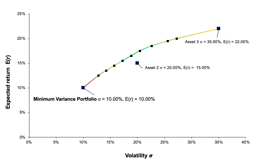
The pioneering work of Henry Markowitz (1952) depicted the effect of diversification by analyzing the portfolio asset allocation in terms of risk and (expected) return. Since unsystematic risk (specific risk) can be neutralized, investors will not receive an additional return. Systematic risk (market risk) is the component that the market rewards. Diversification is then at the heart of asset allocation as emphasized by Modern Portfolio Theory (MPT). The academic literature has since then delved deeper on the analysis of the optimal number of assets to hold in a well-diversified portfolio. We list below some notable contributions worth mentioning:
- Elton and Gruber (1977), Evans and Archer (1968), Tole (1982) and Statman (1987) among others delved deeper into the optimal number of assets to hold to generate the best risk and return portfolio. There is no consensus on the optimal number of assets to select.
- Evans and Archer (1968) depicted that the best results are achieved with 8-10 assets, while raising doubts about portfolios with number of assets above the threshold. Statman (1987) concluded that at least thirty to forty stocks should be included in a portfolio to achieve the portfolio diversification.
Lhabitant and Learned (2002) also mention the concept of naive diversification (also known as “1/N heuristics”) is an allocation strategy where the investor split the overall fund available is distributed into same. Naive diversification seeks to spread asset risk evenly in the portfolio to reduce overall risk. However, the authors mention important considerations for naïve/Markowitz optimization:
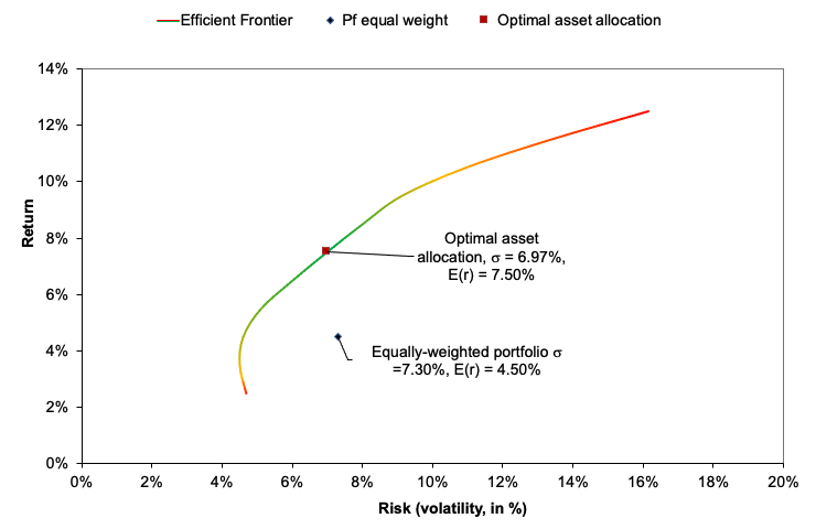
- Drawback of naive diversification: since it doesn’t account for correlation between assets, the allocation will yield a sub-optimal result and the diversification won’t be fully achieved. In practice, naive diversification can result in portfolio allocations that lie on the efficient frontier. On the other hand, mean-variance optimisation, the framework revolving he Modern Portfolio Theory is subject to input sensitivity of the parameters used in the optimization process. On a side note, it is worth mentioning that naive diversification is a good starting point, better than gut feeling. It simplifies allocation process while also benefiting by some degree of risk diversification.
- Non-normality of distribution of returns: hedge funds exhibit non-normal returns (fat tails and skewness). Those higher statistical moments are important for investors allocation but are disregarded in a mean-variance framework.
- Econometric difficulties arising from hedge fund data in an optimizer framework. Mean-variance optimisers tend to consider historical return and risk, covariances as an acceptable point to assess future portfolio performance. Applied in a construction of a hedge fund portfolio, it becomes even more difficult to derive the expected return, correlation, and standard deviation for each fund since data is scarcer and more difficult to obtain. Add to that the instability of the hedge funds returns and the non-linearity of some strategies which complicates the evaluation of a hedge fund portfolio.
- Operational risk arising from fund selection and implementation of the constraints in an optimiser software. Since some parameters are qualitative (i.e., lock up period, minimum investment period), these optimisers tool find it hard to incorporate these types of constraints in the model.
Conclusion
Due to entry restrictions, data scarcity, and a lack of meaningful benchmarks, hedge fund investing is difficult. The paper analyses in greater depth the optimal number of hedge funds to include in a diversified portfolio. According to the authors, adding funds naively to a portfolio tends to lower overall standard deviation and downside risk. In this context, diversification should be improved if the marginal benefit of adding a new asset to a portfolio exceeds its marginal cost.
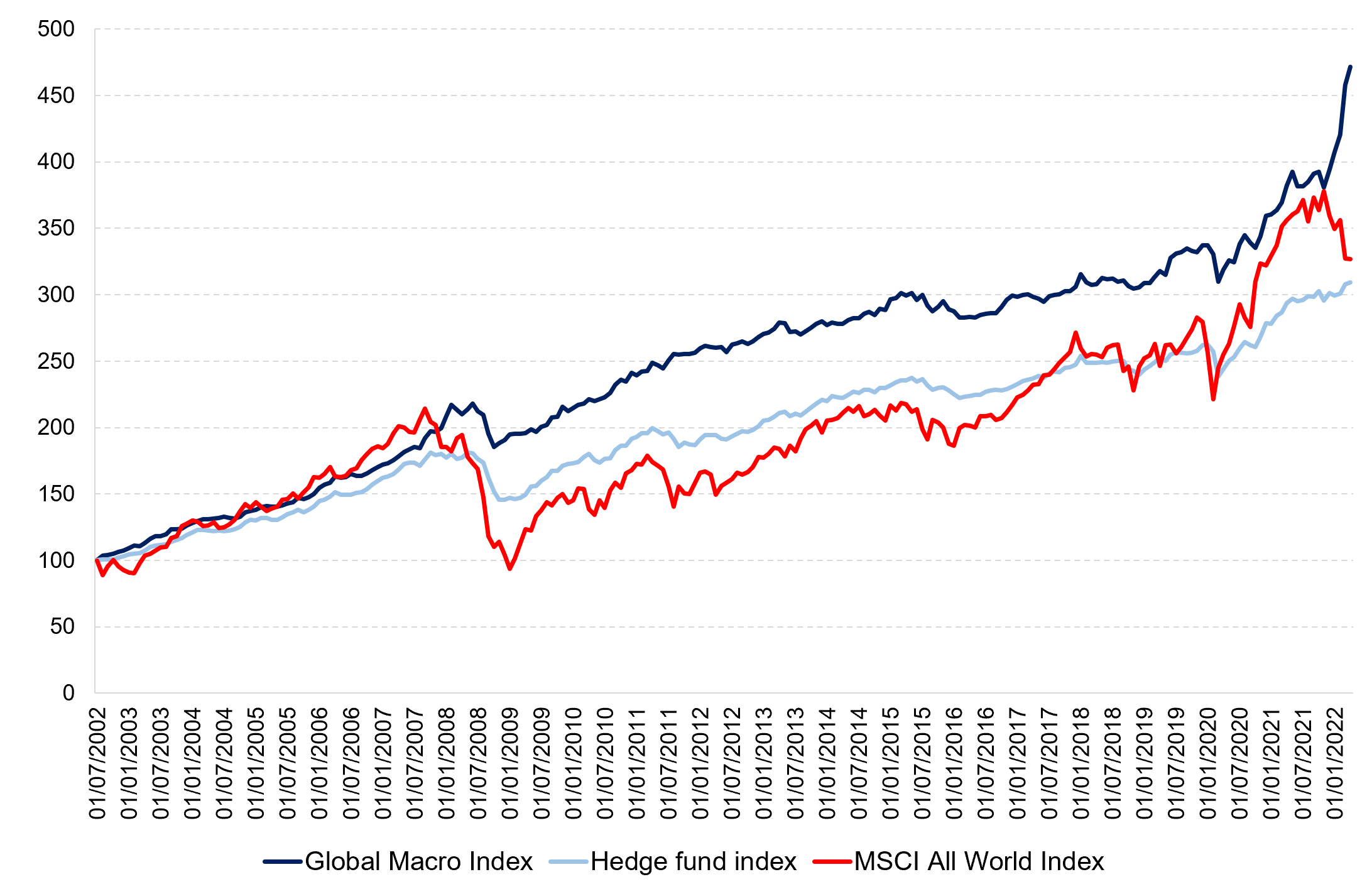
The authors reiterate that investors should not invest “naively” in hedge funds due to their inherent risk. The impact of naive diversification on the portfolio’s skewness, kurtosis, and overall correlation structure can be significant. Hedge fund portfolios should account for this complexity and examine the effect of adding a hedge fund to a well-balanced portfolio, taking into account higher statistical moments to capture the allocation’s impact on portfolio construction. Naive diversification is subject to the selection bias. In the 1990s, the most appealing hedge fund strategy was global macro, although the long/short equity strategy acquired popularity in the late 1990s. This would imply that allocations will be tilted towards these two strategies overall.
The answer to the title of the research paper? Hedge funds portfolios should hold between 15 and 40 underlying funds, while most diversification benefits are reached when accounting with 5 to 10 hedge funds in the portfolio.
Why should I be interested in this post?
The purpose of portfolio management is to maximise returns on the entire portfolio, not just on one or two stocks. By monitoring and maintaining your investment portfolio, you can accumulate a substantial amount of wealth for a range of financial goals, such as retirement planning. This article facilitates comprehension of the fundamentals underlying portfolio construction and investing. Understanding the risk/return profiles, trading strategy, and how to incorporate hedge fund strategies into a diversified portfolio can be of great interest to investors.
Related posts on the SimTrade blog
▶ Youssef LOURAOUI Introduction to Hedge Funds
▶ Youssef LOURAOUI Equity market neutral strategy
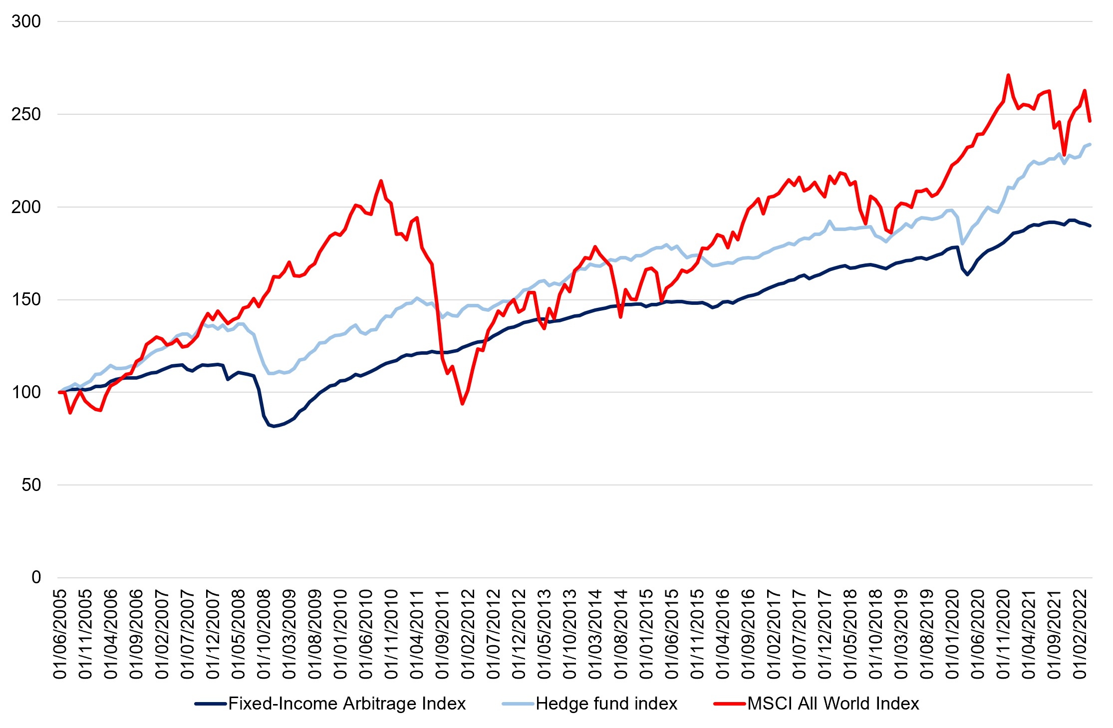
▶ Youssef LOURAOUI Fixed income arbitrage strategy
▶ Youssef LOURAOUI Global macro strategy
▶ Youssef LOURAOUI Long/short equity strategy
▶ Youssef LOURAOUI Portfolio
Useful resources
Academic research
Elton, E., and M. Gruber (1977). “Risk Reduction and Portfolio Size: An Analytical Solution.” Journal of Business, 50. pp. 415-437.
Evans, J.L., and S.H. Archer (1968). “Diversification and the Reduction of Dispersion: An Empirical Analysis”. Journal of Finance, 23. pp. 761-767.
Lhabitant, François S., Learned Mitchelle (2002). “Hedge fund diversification: how much is enough?” Journal of Alternative Investments. pp. 23-49.
Markowitz, H.M (1952). “Portfolio Selection.” The Journal of Finance, 7, pp. 77-91.
Statman, M. (1987). “How many stocks make a diversified portfolio?”, Journal of Financial and Quantitative Analysis , pp. 353-363.
Tole T. (1982). “You can’t diversify without diversifying”, Journal of Portfolio Management, 8, pp. 5-11.
About the author
The article was written in January 2023 by Youssef LOURAOUI (Bayes Business School, MSc. Energy, Trade & Finance, 2021-2022).


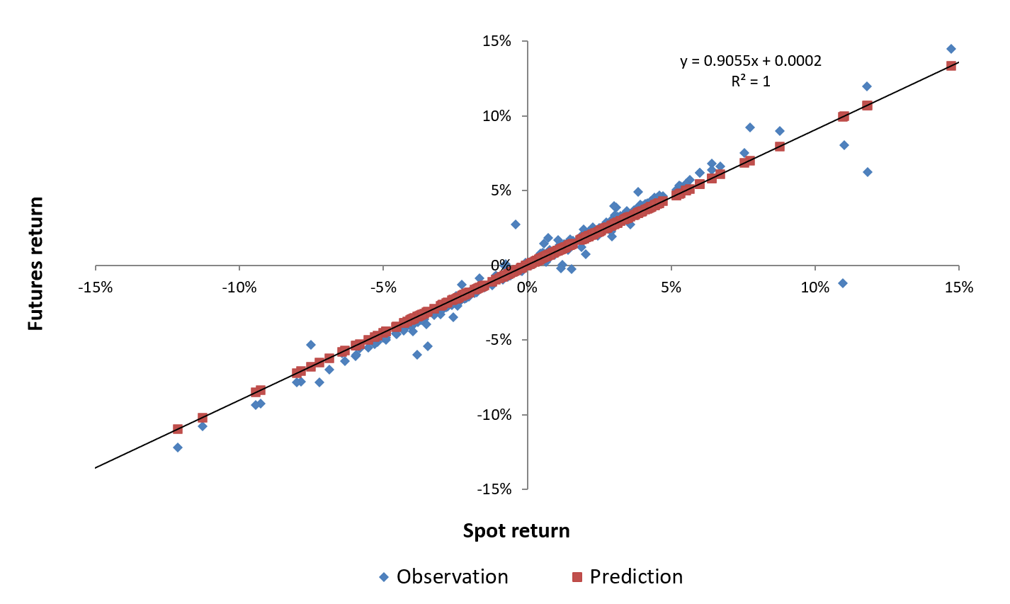
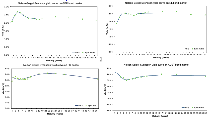
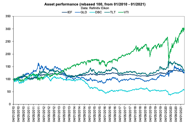
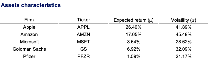
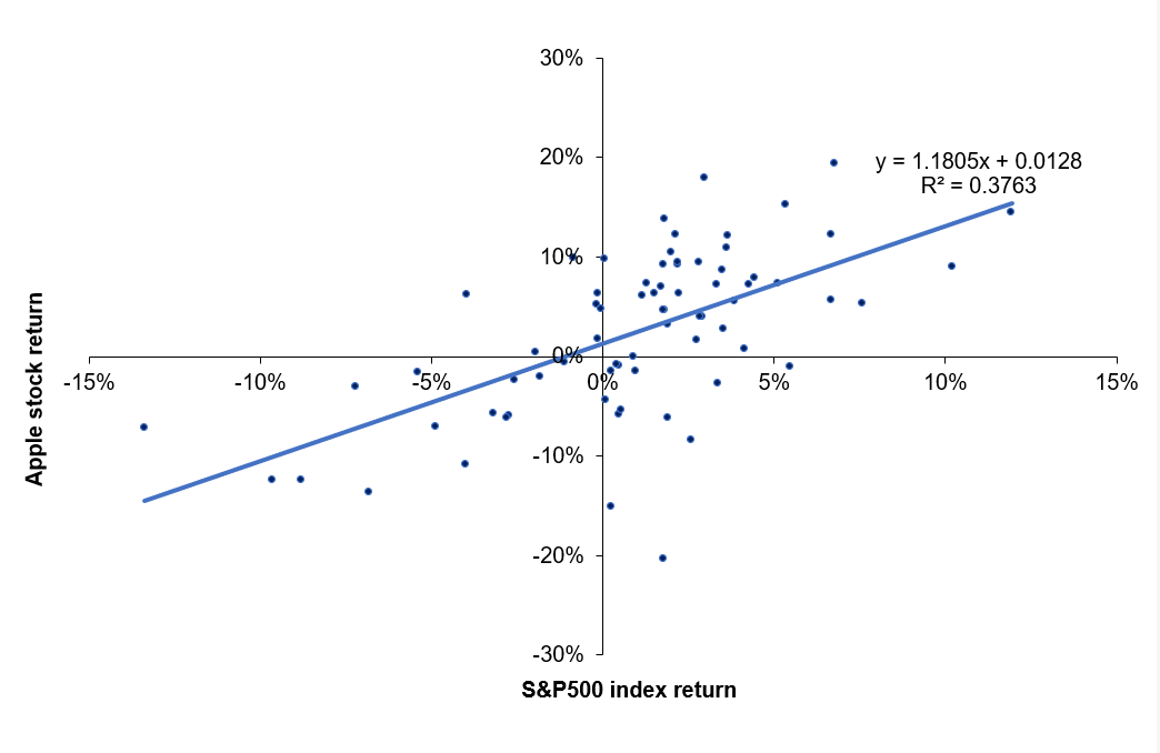
 Source: computation by the author (data: Refinitiv Eikon).
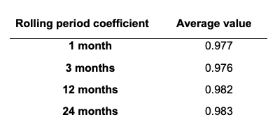
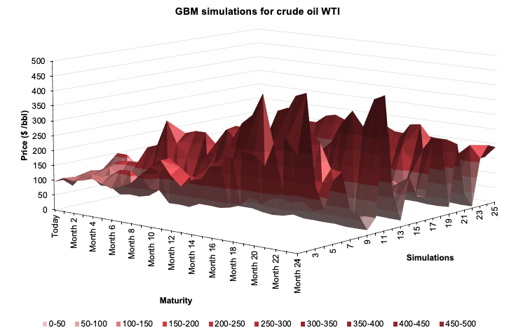
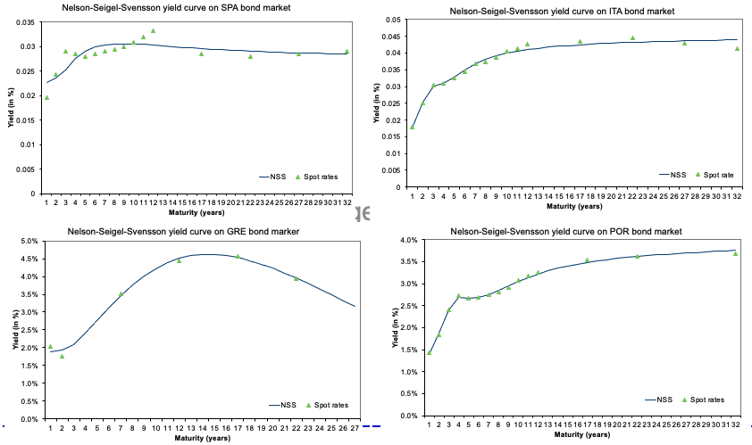
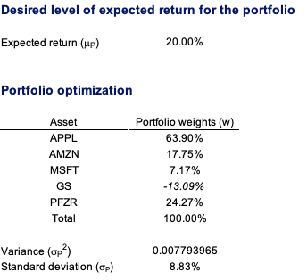
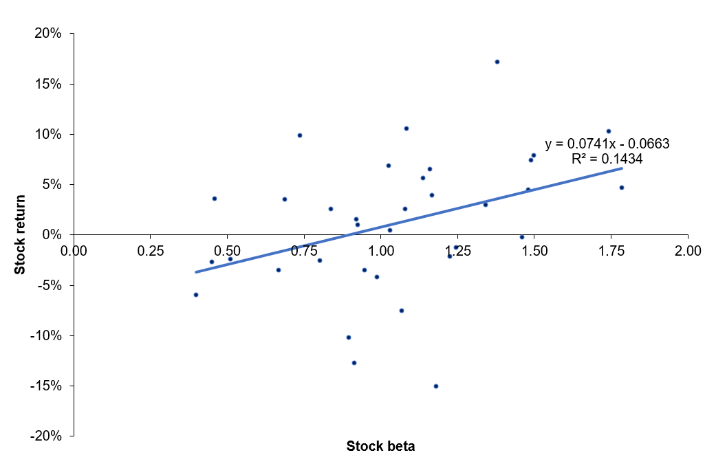
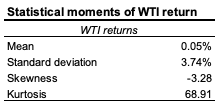
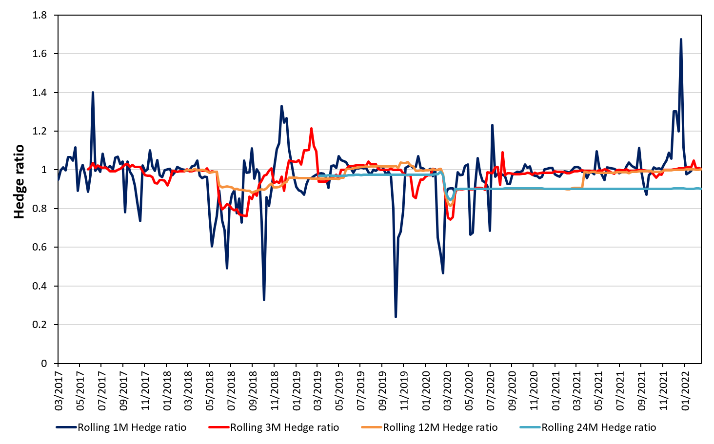
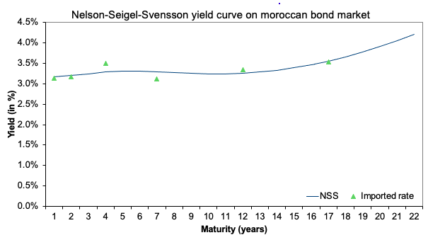
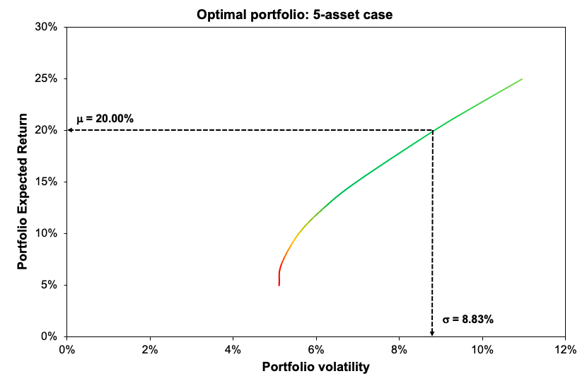
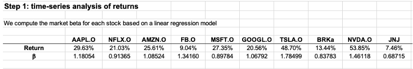
 Source: computation by the author (Data: Refinitiv Eikon).
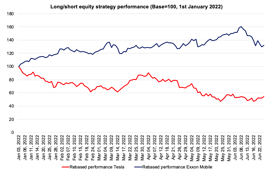
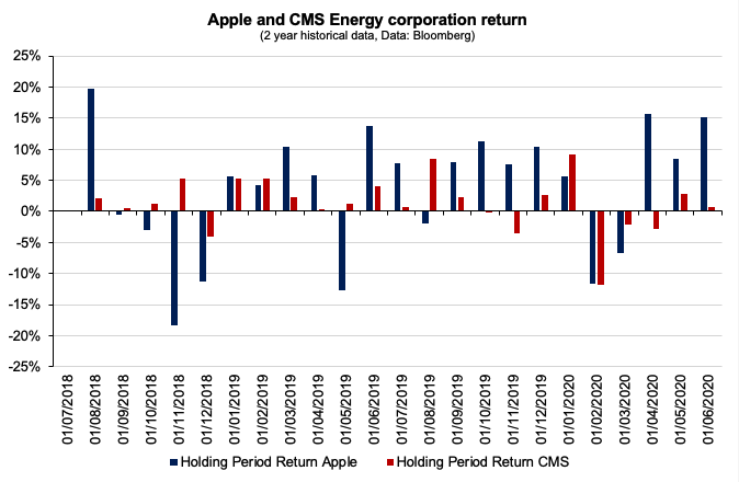
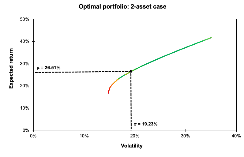
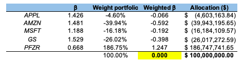 Source: computation by the author (Data: Bloomberg)
 Source: computation by the author. (Data: Reuters Eikon)


 Source: computation by the author.
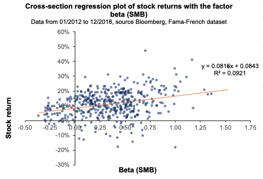 Source: computation by the author.
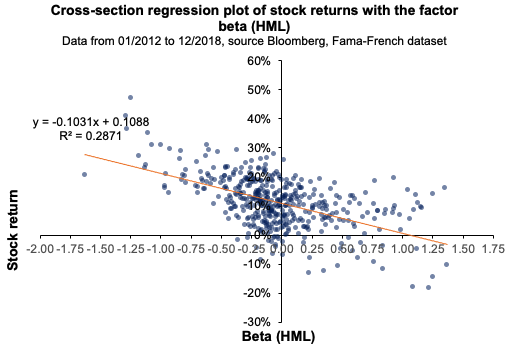 Source: computation by the author.
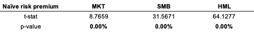 Source: computation by the author.
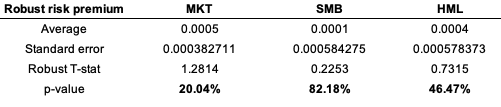 Source: computation by the author.
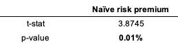 Source: computation by the author.
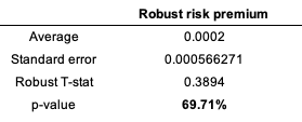 Source: computation by the author.
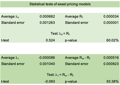 Source: computation by the author.
 Source: computation by the author.
 Source : computation by the author.
 Source: computation by the author.