Arbitrage Pricing Theory (APT)

January 2, 2023 by Youssef LOURAOUI

Arbitrage Pricing Theory (APT)

In this article, Youssef LOURAOUI (Bayes Business School, MSc. Energy, Trade & Finance, 2021-2022) presents the concept of arbitrage portfolio, a pillar concept in asset pricing theory.

This article is structured as follows: we present an introduction for the notion of arbitrage portfolio in the context of asset pricing, we present the assumptions and the mathematical foundation of the model and we then illustrate a practical example to complement this post.

Introduction

Arbitrage pricing theory (APT) is a method of explaining asset or portfolio returns that differs from the capital asset pricing model (CAPM). It was created in the 1970s by economist Stephen Ross. Because of its simpler assumptions, arbitrage pricing theory has risen in favor over the years. However, arbitrage pricing theory is far more difficult to apply in practice since it requires a large amount of data and complicated statistical analysis.The following points should be kept in mind when understanding this model:

Arbitrage is the technique of buying and selling the same item at two different prices at the same time for a risk-free profit.
Arbitrage pricing theory (APT) in financial economics assumes that market inefficiencies emerge from time to time but are prevented from occurring by the efforts of arbitrageurs who discover and instantly remove such opportunities as they appear.
APT is formalized through the use of a multi-factor formula that relates the linear relationship between the expected return on an asset and numerous macroeconomic variables.

The concept that mispriced assets can generate short-term, risk-free profit opportunities is inherent in the arbitrage pricing theory. APT varies from the more traditional CAPM in that it employs only one factor. The APT, like the CAPM, assumes that a factor model can accurately characterize the relationship between risk and return.

Assumptions of the APT model

Arbitrage pricing theory, unlike the capital asset pricing model, does not require that investors have efficient portfolios. However, the theory is guided by three underlying assumptions:

Systematic factors explain asset returns.
Diversification allows investors to create a portfolio of assets that eliminates specific risk.
There are no arbitrage opportunities among well-diversified investments. If arbitrage opportunities exist, they will be taken advantage of by investors.

To have a better grasp on the asset pricing theory behind this model, we can recall in the following part the foundation of the CAPM as a complementary explanation for this article.

Capital Asset Pricing Model (CAPM)

William Sharpe, John Lintner, and Jan Mossin separately developed a key capital market theory based on Markowitz’s work: the Capital Asset Pricing Model (CAPM). The CAPM was a huge evolutionary step forward in capital market equilibrium theory, since it enabled investors to appropriately value assets in terms of systematic risk, defined as the market risk which cannot be neutralized by the effect of diversification. In their derivation of the CAPM, Sharpe, Mossin and Litner made significant contributions to the concepts of the Efficient Frontier and Capital Market Line. The seminal contributions of Sharpe, Litner and Mossin would later earn them the Nobel Prize in Economics in 1990.

The CAPM is based on a set of market structure and investor hypotheses:

There are no intermediaries
There are no limits (short selling is possible)
Supply and demand are in balance
There are no transaction costs
An investor’s portfolio value is maximized by maximizing the mean associated with projected returns while reducing risk variance
Investors have simultaneous access to information in order to implement their investment plans
Investors are seen as “rational” and “risk averse”.

Under this framework, the expected return of a given asset is related to its risk measured by the beta and the market risk premium:

CAPM risk beta relation

Where :

E(r_i) represents the expected return of asset i
r_f the risk-free rate
β_i the measure of the risk of asset i
E(r_m) the expected return of the market
E(r_m)- r_f the market risk premium.

In this model, the beta (β) parameter is a key parameter and is defined as:

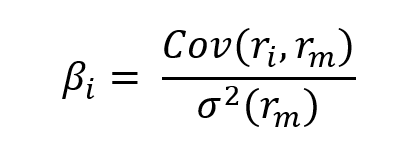
CAPM beta formula

Where:

Cov(r_i, r_m) represents the covariance of the return of asset i with the return of the market
σ²(r_m) is the variance of the return of the market.

The beta is a measure of how sensitive an asset is to market swings. This risk indicator aids investors in predicting the fluctuations of their asset in relation to the wider market. It compares the volatility of an asset to the systematic risk that exists in the market. The beta is a statistical term that denotes the slope of a line formed by a regression of data points comparing stock returns to market returns. It aids investors in understanding how the asset moves in relation to the market. According to Fama and French (2004), there are two ways to interpret the beta employed in the CAPM:

According to the CAPM formula, beta may be thought in mathematical terms as the slope of the regression between the asset return and the market return. Thus, beta quantifies the asset sensitivity to changes in the market return.
According to the beta formula, it may be understood as the risk that each dollar invested in an asset adds to the market portfolio. This is an economic explanation based on the observation that the market portfolio’s risk (measured by σ²(r_m)) is a weighted average of the covariance risks associated with the assets in the market portfolio, making beta a measure of the covariance risk associated with an asset in comparison to the variance of the market return.

Mathematical foundations

The APT can be described formally by the following equation

APT expected return formula

Where

E(r_p) represents the expected return of portfolio p
r_f the risk-free rate
β_k the sensitivity of the return on portfolio p to the k^th factor (f_k)
λ_k the risk premium for the k^th factor (f_k)
K the number of risk factors

Richard Roll and Stephen Ross found out that the APT can be sensible to the following factors:

Expectations on inflation
Industrial production (GDP)
Risk premiums
Term structure of interest rates

Furthermore, the researchers claim that an asset will have varied sensitivity to the elements indicated above, even if it has the same market factor as described by the CAPM.

Application

For this specific example, we want to understand the asset price behavior of two equity indexes (Nasdaq for the US and Nikkei for Japan) and assess their sensitivity to different macroeconomic factors. We extract a time series for Nasdaq equity index prices, Nikkei equity index prices, USD/CHY FX spot rate and US term structure of interest rate (10y-2y yield spread) from the FRED Economics website, a reliable source for macroeconomic data for the last two decades.

The first factor, which is the USD/CHY (US Dollar/Chinese Renminbi Yuan) exchange rate, is retained as the primary factor to explain portfolio return. Given China’s position as a major economic player and one of the most important markets for the US and Japanese corporations, analyzing the sensitivity of US and Japanese equity returns to changes in the USD/CHY Fx spot rate can help in understanding the market dynamics underlying the US and Japanese equity performance. For instance, Texas Instrument, which operates in the sector of electronics and semiconductors, and Nike both have significant ties to the Chinese market, with an overall exposure representing approximately 55% and 18%, respectively (Barrons, 2022). In the example of Japan, in 2017 the Japanese government invested 117 billion dollars in direct investment in northern China, one of the largest foreign investments in China. Similarly, large Japanese listed businesses get approximately 18% of their international revenues from the Chinese market (The Economist, 2019).

The second factor, which is the 10y-2y yield spread, is linked to the shape of the yield curve. A yield curve that is inverted indicates that long-term interest rates are lower than short-term interest rates. The yield on an inverted yield curve decreases as the maturity date approaches. The inverted yield curve, also known as a negative yield curve, has historically been a reliable indicator of a recession. Analysts frequently condense yield curve signals to the difference between two maturities. According to the paper of Yu et al. (2017), there is a significant link between the effects of varying degrees of yield slope with the performance of US equities between 2006 and 2012. Regardless of market capitalization, the impact of the higher yield slope on stock prices was positive.

The APT applied to this example can be described formally by the following equation:

APT expected return formula example

Where

E(r_p) represents the expected return of portfolio p
r_f the risk-free rate
β_{p, Chinese FX} the sensitivity of the return on portfolio p to the USD/CHY FX spot rate
β_{p, US spread} the sensitivity of the return on portfolio p to the US term structure
λ_{Chinese FX} the risk premium for the FX risk factor
λ_{US spread} the risk premium for the interest rate risk factor

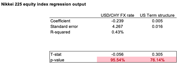
We run a first regression of the Nikkei Japanese equity index returns onto the macroeconomic variables retained in this analysis. We can highlight the following: Both factors are not statistically significant at a 10% significance level, indicating that the factors have poor predictive power in explaining Nikkei 225 returns over the last two decades. The model has a low R2, equivalent to 0.48%, which indicates that only 0.48% of the behavior of Nikkei performance can be attributed to the change in USD/CHY FX spot rate and US term structure of the yield curve (Table 1).

Table 1. Nikkei 225 equity index regression output.
Time-series regression
Source: computation by the author (Data: FRED Economics)

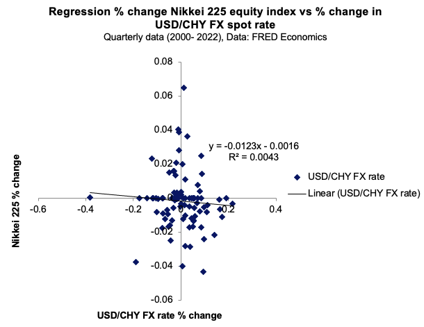
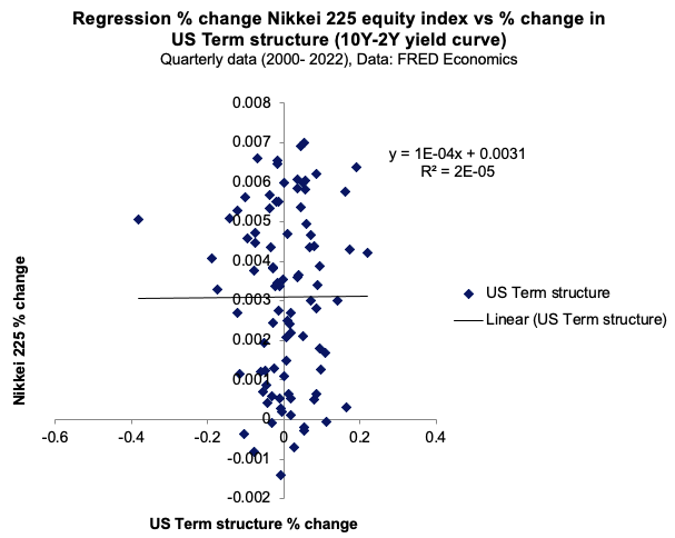
Figure 1 and 2 captures the linear relationship between the USD/CHY FX spot rate and the US term structure with respect to the Nikkei equity index.

Figure 1. Relationship between the USD/CHY FX spot rate with respect to the Nikkei 225 equity index.
Time-series regression
Source: computation by the author (Data: FRED Economics)

Figure 2. Relationship between the US term structure with respect to the Nikkei 225 equity index.
Time-series regression
Source: computation by the author (Data: FRED Economics)

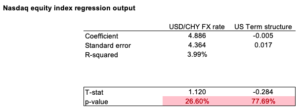
We conduct a second regression of the Nasdaq US equity index returns on the retained macroeconomic variables. We may emphasize the following: Both factors are not statistically significant at a 10% significance level, indicating that they have a limited ability to predict Nasdaq returns during the past two decades. The model has a low R2 of 4.45%, indicating that only 4.45% of the performance of the Nasdaq can be attributable to the change in the USD/CHY FX spot rate and the US term structure of the yield curve (Table 2).

Table 2. Nasdaq equity index regression output.
Time-series regression
Source: computation by the author (Data: FRED Economics)

Figure 3 and 4 captures the linear relationship between the USD/CHY FX spot rate and the US term structure with respect to the Nasdaq equity index.

Figure 3. Relationship between the USD/CHY FX spot rate with respect to the Nasdaq equity index.
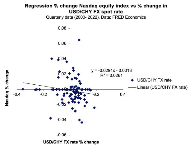
Time-series regression
Source: computation by the author (Data: FRED Economics)

Figure 4. Relationship between the US term structure with respect to the Nasdaq equity index.
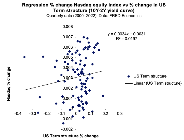
Time-series regression
Source: computation by the author (Data: FRED Economics)

Applying APT

We can create a portfolio with similar factor sensitivities as the Arbitrage Portfolio by combining the first two index portfolios (with a Nasdaq Index weight of 40% and a Nikkei Index weight of 60%). This is referred to as the Constructed Index Portfolio. The Arbitrage portfolio will have a full weighting on US equity index (100% Nasdaq equity index). The Constructed Index Portfolio has the same systematic factor betas as the Arbitrage Portfolio, but has a higher expected return (Table 3).

Table 3. Index, constructed and Arbitrage portfolio return and sensitivity table. img_SimTrade_portfolio_sensitivity
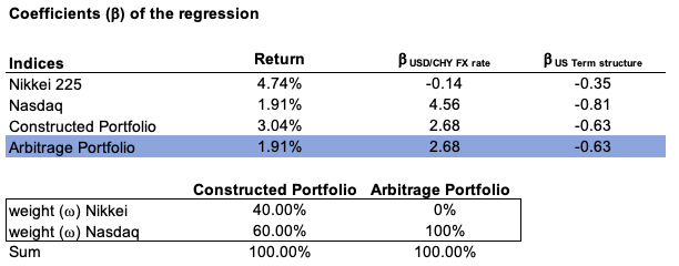
Source: computation by the author (Data: FRED Economics)

As a result, the Arbitrage portfolio is overvalued. We will then buy shares of the Constructed Index Portfolio and use the profits to sell shares of the Arbitrage Portfolio. Because every investor would sell an overvalued portfolio and purchase an undervalued portfolio, any arbitrage profit would be wiped out.

Excel file for the APT application

You can find below the Excel spreadsheet that complements the example above.

Why should I be interested in this post?

In the CAPM, the factor is the market factor representing the global uncertainty of the market. In the late 1970s, the portfolio management industry aimed to capture the market portfolio return, but as financial research advanced and certain significant contributions were made, this gave rise to other factor characteristics to capture some additional performance. Analyzing the historical contributions that underpins factor investing is fundamental in order to have a better understanding of the subject.

Useful resources

Academic research

Lintner, J. (1965) The Valuation of Risk Assets and the Selection of Risky Investments in Stock Portfolios and Capital Budgets. The Review of Economics and Statistics 47(1): 13-37.

Lintner, J. (1965) Security Prices, Risk and Maximal Gains from Diversification. The Journal of Finance 20(4): 587-615.

Roll, Richard & Ross, Stephen. (1995). The Arbitrage Pricing Theory Approach to Strategic Portfolio Planning. Financial Analysts Journal 51, 122-131.

Ross, S. (1976) The arbitrage theory of capital asset pricing Journal of Economic Theory 13(3), 341-360.

Sharpe, W.F. (1963) A Simplified Model for Portfolio Analysis. Management Science 9(2): 277-293.

Sharpe, W.F. (1964) Capital Asset Prices: A theory of Market Equilibrium under Conditions of Risk. The Journal of Finance 19(3): 425-442.

Yu, G., P. Fuller, D. Didia (2013) The Impact of Yield Slope on Stock Performance Southwestern Economic Review 40(1): 1-10.

Business Analysis

Barrons (2022) Apple, Nike, and 6 Other Companies With Big Exposure to China.

The Economist (2019) Japan Inc has thrived in China of late.

Investopedia (2022) Arbitrage Pricing Theory: It’s Not Just Fancy Math.

Time series

FRED Economics (2022) Chinese Yuan Renminbi to U.S. Dollar Spot Exchange Rate (DEXCHUS).

FRED Economics (2022) 10-Year Treasury Constant Maturity Minus 2-Year Treasury Constant Maturity (T10Y2Y).

FRED Economics (2022) NASDAQ Composite Index (NASDAQCOM).

FRED Economics (2022) Nikkei Stock Average, Nikkei 225 (NIKKEI225).

About the author

The article was written in January 2023 by Youssef LOURAOUI (Bayes Business School, MSc. Energy, Trade & Finance, 2021-2022).

Fama-MacBeth two-step regression method: the case of K risk factors

December 12, 2022 by Youssef LOURAOUI

Fama-MacBeth two-step regression method: the case of K risk factors

This article is structured as follows: we introduce the Fama-MacBeth two-step regression method. Then, we present the mathematical foundation that underpins their approach for K risk factors. We provide an illustration for the 3-factor mode developed by Fama and French (1993).

Introduction

Risk factors are frequently employed to explain asset returns in asset pricing theories. These risk factors may be macroeconomic (such as consumer inflation or unemployment) or microeconomic (such as firm size or various accounting and financial metrics of the firms). The Fama-MacBeth two-step regression approach found a practical way for measuring how correctly these risk factors explain asset or portfolio returns. The aim of the model is to determine the risk premium associated with the exposure to these risk factors.

The first step is to regress the return of every asset against one or more risk factors using a time-series approach. We obtain the return exposure to each factor called the “betas” or the “factor exposures” or the “factor loadings”.

The second step is to regress the returns of all assets against the asset betas obtained in Step 1 using a cross-section approach. We obtain the risk premium for each factor. Then, Fama and MacBeth assess the expected premium over time for a unit exposure to each risk factor by averaging these coefficients once for each element.

Mathematical foundations

We describe below the mathematical foundations for the Fama-MacBeth regression method for a K-factor application. In the analysis, we investigated the Fame-French three factor model in order to understand their significance as a fundamental driver of returns for investors under the Fama-MacBeth framework.

The model considers the following inputs:

The return of N assets denoted by R_i for asset i observed every day over the time period [0, T].
The risk factors denoted by F_k for k equal from 1 to K.

Step 1: time-series analysis of returns

For each asset i from 1 to N, we estimate the following linear regression model:

Fama-French time-series regression

From this model, we obtain the β_{i, Fk} which is the beta associated with the k^th risk factor.

Step 2: cross-sectional analysis of returns

For each period t from 1 to T, we estimate the following linear regression model:

Fama-French cross-sectional regression

Application: the Fama-French 3-Factor model

The Fama-French 3-factor model is an illustration of Fama-MacBeth two-step regression method in the case of K risk factors (K=3). The three factors are the market (MKT) factor, the small minus big (SMB) factor, and the high minus low (HML) factor. The SMB factor measures the difference in expected returns between small and big firms (in terms of market capitalization). The HML factor measures the difference in expected returns between value stocks and growth stock.

The model considers the following inputs:

The return of N assets denoted by R_i for asset i observed every day over the time period [0, T].
The risk factors denoted by F_MKT associated to the MKT risk factor, F_SMB associated to the MKT risk factor which measures the difference in expected returns between small and big firms (in terms of market capitalization) and F_HML associated to 𝐻𝑀𝐿 (“High Minus Low”) which measures the difference in expected returns between value stocks and growth stock

Step 1: time-series regression

img_SimTrade_Fama_French_time_series_regression

Step 2: cross-sectional regression

img_SimTrade_Fama_French_cross_sectional_regression

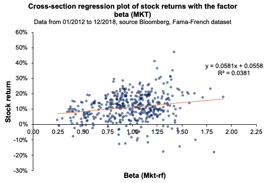
Figure 1 represents for a given period the cross-sectional regression of the return of all individual assets with respect to their estimated individual beta for the MKT factor.

Figure 1. Cross-sectional regression for the market factor.
Cross-section regression for the MKT factor Source: computation by the author.

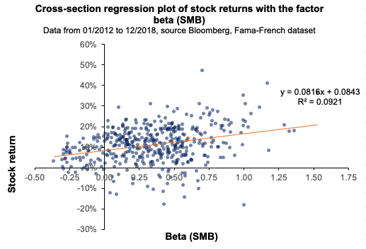
Figure 2 represents for a given period the cross-sectional regression of the return of all individual assets with respect to their estimated individual beta for the SMB factor.

Figure 2. Cross-sectional regression for the SMB factor.
Cross-section regression for the SMB factor Source: computation by the author.

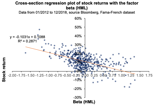
Figure 3 represents for a given period the cross-sectional regression of the return of all individual assets with respect to their estimated individual beta for the SMB factor.

Figure 3. Cross-sectional regression for the HML factor.
Cross-section regression for the HML factor Source: computation by the author.

Empirical study of the Fama-MacBeth regression

Fama-MacBeth seminal paper (1973) was based on an analysis of the market factor by assessing constructed portfolios of similar betas ranked by increasing values. This approach helped to overcome the shortcoming regarding the stability of the beta and correct for conditional heteroscedasticity derived from the computation of the betas for individual stocks. They performed a second time the cross-sectional regression of monthly portfolio returns based on equity betas to account for the dynamic nature of stock returns, which help to compute a robust standard error and assess if there is any heteroscedasticity in the regression. The conclusion of the seminal paper suggests that the beta is “dead”, in the sense that it cannot explain returns on its own (Fama and MacBeth, 1973).

Empirical study: Stock approach for a K-factor model

We collected a sample of 440 significant firms’ end-of-day stock prices in the US economy from January 3, 2012 to December 31, 2021. We calculated daily returns for each stock as well as the factor used in this analysis. We chose the S&P500 index to represent the market since it is an important worldwide stock benchmark that captures the US equities market.

Time-series regression

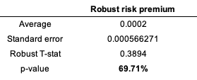
To assess the multi-factor regression, we used the Fama-MacBeth 3-factor model as the main factors assessed in this analysis. We regress the average returns for each stock against their factor betas. The first regression is statistically tested. This time-series regression is run on a subperiod of the whole period from January 03, 2012, to December 31, 2018. We use a t-statistic to explain the regression’s behavior. Because the p-value is in the rejection zone (less than the significance level of 5%), we can conclude that the factors can first explain an investor’s returns. However, as we will see later in the article, when we account for a second regression as proposed by Fama and MacBeth, the factors retained in this analysis are not capable of explaining the return on asset returns on its own. The stock approach produces statistically significant results in time-series regression at 10%, 5%, and even 1% significance levels. As shown in Table 1, the p-value is in the rejection range, indicating that the factors are statistically significant.

Table 1. Time-series regression t-statistic result.
Cross-section regression Source: computation by the author.

Cross-sectional regression

Over a second period from January 04, 2019, to December 31, 2021, we compute the dynamic regression of returns at each data point in time with respect to the betas computed in Step 1.

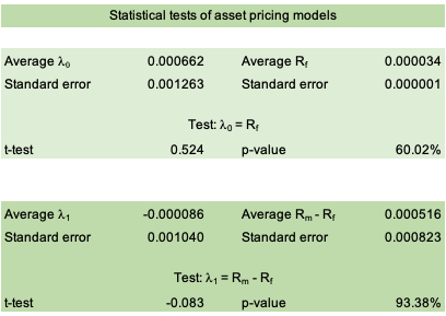
That being said, when the results are examined using cross-section regression, they are not statistically significant, as indicated by the p-value in Table 2. We are unable to reject the null hypothesis. The premium investors are evaluating cannot be explained solely by the factors assessed. This suggests that factors retained in the analysis fail to adequately explain the behavior of asset returns. These results are consistent with the Fama-MacBeth article (1973).

Table 2. Cross-section regression t-statistic result.
Source: computation by the author.

Excel file

You can find below the Excel spreadsheet that complements the explanations covered in this article.

Why should I be interested in this post?

Fama-MacBeth made a significant contribution to the field of econometrics. Their findings cleared the way for asset pricing theory to gain traction in academic literature. The Capital Asset Pricing Model (CAPM) is far too simplistic for a real-world scenario since the market factor is not the only source that drives returns; asset return is generated from a range of factors, each of which influences the overall return. This framework helps in capturing other sources of return.

Useful resources

Academic research

Brooks, C., 2019. Introductory Econometrics for Finance (4th ed.). Cambridge: Cambridge University Press. doi:10.1017/9781108524872

Fama, E. F., MacBeth, J. D., 1973. Risk, Return, and Equilibrium: Empirical Tests. Journal of Political Economy, 81(3), 607–636.

Roll R., 1977. A critique of the Asset Pricing Theory’s test, Part I: On Past and Potential Testability of the Theory. Journal of Financial Economics, 1, 129-176.

American Finance Association & Journal of Finance (2008) Masters of Finance: Eugene Fama (YouTube video)

About the author

The article was written in December 2022 by Youssef LOURAOUI (Bayes Business School, MSc. Energy, Trade & Finance, 2021-2022).

Fama-MacBeth regression method: the stock approach vs the portfolio approach

December 12, 2022 by Youssef LOURAOUI

Fama-MacBeth regression method: the stock approach vs the portfolio approach

In this article, Youssef LOURAOUI (Bayes Business School, MSc. Energy, Trade & Finance, 2021-2022) presents the Fama-MacBeth regression method used to test asset pricing models and addresses the difference when applying the regression method on individual stocks or portfolios composed of stocks with similar betas.

This article is structured as follow: we introduce the Fama-MacBeth testing method. Then, we present the mathematical foundation that underpins their approach. We conduct an empirical analysis on both the stock and the portfolio approach. We conclude with a discussion on econometric issues.

Introduction

As a reminder, the Fama-MacBeth regression method is composed on two steps: step 1 with a time-series regression and step 2 with a cross-section regression.

The first step is to regress the return of every stock against one or more risk factors using a time-series regression. We obtain the return exposure to each factor called the “betas” or the “factor exposures” or the “factor loadings”.

The second step is to regress the returns of all stocks against the asset betas obtained in the first step using a cross-section regression for different periods. We obtain the risk premium for each factor used to test the asset pricing model.

The implementation of this method can be done with individual stocks or with portfolios of stocks as proposed by Fama and MacBeth (1973). Their argument is the better stability of the beta when considering portfolios. In this article we illustrate the difference with the two implementations.

Fama and MacBeth (1973) implemented with individual stocks

We downloaded a sample of daily prices of stocks composing the S&P500 index over the period from January 03, 2012, to December 31, 2021 (we selected the stocks present from the beginning to the end of the period reducing our sample from 500 to 440 stocks). We computed daily returns for each stock and for the market factor retained in this study. To represent the market, we chose the S&P500 index, an important global stock benchmark capturing the US equity market.

The procedure to derive the Fama-MacBeth regression using the stock approach can be achieved as follow:

Step 1: time-series regression

We compute the beta of the stocks with respect to the market factor for the period covered (time-series regression). We estimate the beta of each stock related to the S&P500 index. The beta is computed as the slope of the linear regression of the stock return on the market return (S&P500 index return). This time-series regression is run on a subperiod of the whole period from January 03, 2012, to December 31, 2018.

Step 2: cross-sectional regression

Over a second period from January 04, 2019, to December 31, 2021, we compute the dynamic regression of returns at each data point in time with respect to the betas computed in Step 1.

With this procedure, we obtain a risk premium that would represent the relationship between the stock returns at each data point in time with their respective beta for the sample analyzed.

Test the statistical significance of the results obtained from the regression

Results in the time-series regression using the stock approach are statistically significant. As shown in Table 1, the p-value is in the rejection area, which implies that the factor that the market factor can be considered as a driver of return.

Table 1. Time-series regression t-statistic result.
img_SimTrade_Fama_MacBeth_cross_sectional_regression_stat_result Source: computation by the author.

However, when analyzed in the cross-section regression, the results are not statistically significant anymore. As shown in Table 2, the p-value is not in the rejection area. We cannot reject the null hypothesis (H0: non significance of the market factor). Market factor alone cannot explain the premium investors are considering.
This means that the market factor fails to explain properly the behavior of asset returns, which undermines the validity of the CAPM framework. These results are in line with the Fama-MacBeth paper (1973).

Table 2. Cross-section regression t-statistic result.
img_SimTrade_Fama_MacBeth_cross_sectional_regression_stat_result Source: computation by the author.

You can find below the Excel spreadsheet that complements the explanations covered in this part of the article (implementation of the Fama and MacBeth (1973) method with individual stocks).

Fama and MacBeth (1973) implemented with portfolios of stocks

The procedure to derive the Fama-MacBeth regression using the portfolio approach can be achieved as follow:

Step 1: time-series regression

We first compute the beta of the stocks with respect to the market factor for the period covered (time-series regression). We estimate the beta of each stock related to the S&P500 index. The beta is computed as the slope of the linear regression of the stock return on the market return (S&P500 index return). This time-series regression is run on a subperiod of the whole period from January 03, 2012, to December 31, 2015. We build twenty portfolios based on stock betas ranked in ascending order. The betas of the portfolios are then estimated again on a subperiod from January 04, 2016, to December 31, 2018.

It is challenging to maintain beta stability over time. Fama-MacBeth aimed to remedy this shortcoming through its novel technique. However, some issues must be addressed. When betas are calculated using a monthly time series, the statistical noise in the time series is significantly reduced in comparison to shorter time frames (i.e., daily observation). When portfolio betas are constructed, the coefficient becomes considerably more stable than when individual betas are evaluated. This is due to the diversification impact that a portfolio can produce, which considerably reduces the amount of specific risk.

Step 2: cross-sectional regression

Over a second period from January 03, 2019, to December 31, 2021, we compute the dynamic regression of portfolio returns at each data point in time with respect to the betas computed in Step 1.

With this procedure, we obtain a risk premium that would represent the relationship between the portfolio returns at each data point in time with their respective beta for the sample analyzed.

Test the statistical significance of the results obtained from the regression

Results in the cross-section regression using the portfolio approach are not statistically significant. As captured in Table 3, the p-value is not in the rejection area, which implies that the factor is statistically insignificant and that the market factor cannot be considered as a driver of return.

Table 3. Cross-section regression with portfolio approach t-statistic result.
img_SimTrade_Fama_MacBeth_Portfolio_cross_sectional_regression_stat_result Source: computation by the author.

You can find below the Excel spreadsheet that complements the explanations covered in this part of the article (implementation of the Fama and MacBeth (1973) method with portfolios of stocks).

Econometric issues

Errors in data measurement

Because regression uses a sample instead of the entire population, a certain margin of error must be accounted for since the authors derive estimated betas for the sample.

Asset return heteroscedasticity

In econometrics, heteroscedasticity is an important concern since it results in unequal residual variance. This indicates that a time series exhibiting some heteroscedasticity has a non-constant variance, which renders forecasting ineffective because the time series will not revert to its long-run mean.

Asset return autocorrelation

Standard errors in Fama-MacBeth regressions are solely corrected for cross-sectional correlation. This method does not fix the standard errors for time-series autocorrelation. This is typically not a concern for stock trading, as daily and weekly holding periods have modest time-series autocorrelation, whereas autocorrelation is larger over long horizons. This suggests that Fama-MacBeth regression may not be applicable in many corporate finance contexts where project holding durations are typically lengthy.

Why should I be interested in this post?

Useful resources

Academic research

Brooks, C., 2019. Introductory Econometrics for Finance (4th ed.). Cambridge: Cambridge University Press. doi:10.1017/9781108524872

Fama, E. F., MacBeth, J. D., 1973. Risk, Return, and Equilibrium: Empirical Tests. Journal of Political Economy, 81(3), 607–636.

Roll R., 1977. A critique of the Asset Pricing Theory’s test, Part I: On Past and Potential Testability of the Theory. Journal of Financial Economics, 1, 129-176.

American Finance Association & Journal of Finance (2008) Masters of Finance: Eugene Fama (YouTube video)

About the author

The article was written in December 2022 by Youssef LOURAOUI (Bayes Business School, MSc. Energy, Trade & Finance, 2021-2022).

Fama-MacBeth regression method: Analysis of the market factor

December 12, 2022 by Youssef LOURAOUI

In this article, Youssef LOURAOUI (Bayes Business School, MSc. Energy, Trade & Finance, 2021-2022) presents the Fama-MacBeth two-step regression method used to test asset pricing models. The seminal paper by Fama and MacBeth (1973) was based on an investigation of the market factor by evaluating portfolios of stocks with similar betas. In this article I will elaborate on the methodology and assess the statistical significance of the market factor as a fundamental driver of return.

This article is structured as follow: we introduce the Fama-MacBeth testing method used in asset pricing. Then, we present the mathematical foundation that underpins their approach. I then apply the Fama-MacBeth to recent US stock market data. Finally, I expose the limitations of their approach and conclude to discuss the generalization of the original study to other risk factors.

Introduction

The two-step regression method proposed by Fama-MacBeth was originally used in asset pricing to test the Capital Asset Pricing Model (CAPM). In this model, there is only one risk factor determining the variability of returns: the market factor.

The first step is to regress the return of every asset against the risk factor using a time-series approach. We obtain the return exposure to the factor called the “beta” or the “factor exposure” or the “factor loading”.

The second step is to regress the returns of all assets against the asset betas obtained in Step 1 during a given time period using a cross-section approach. We obtain the risk premium associated with the market factor. Then, Fama and MacBeth (1973) assess the expected premium over time for a unit exposure to the risk factor by averaging these coefficients once for each element.

Mathematical foundations

We describe below the mathematical foundations for the Fama-MacBeth two-step regression method.

Step 1: time-series analysis of returns

The model considers the following inputs:

The return of N assets denoted by R_i for asset i observed over the time period [0, T].
The risk factor denoted by F for the market factor impacting the asset returns.

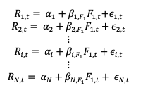
For each asset i (for i varying from 1 to N) we estimate the following time-series linear regression model:

Fama MacBeth time-series regression

From this model, we obtain the following coefficients: α_i and β_i which are specific to asset i.

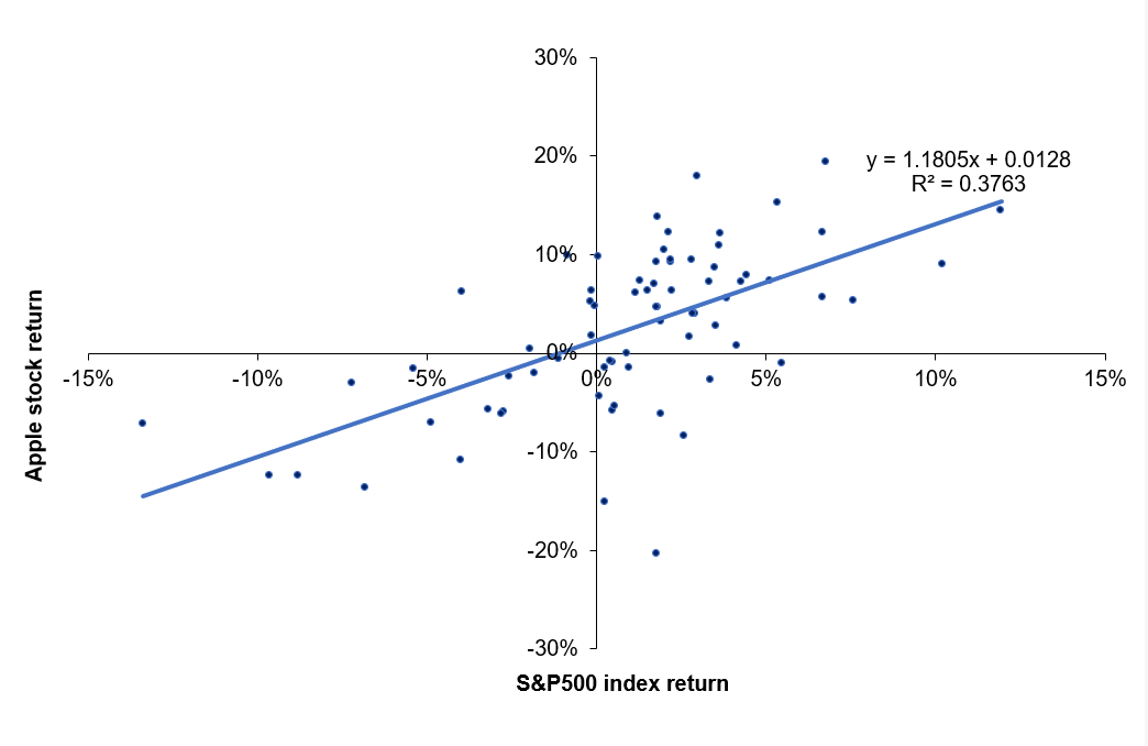
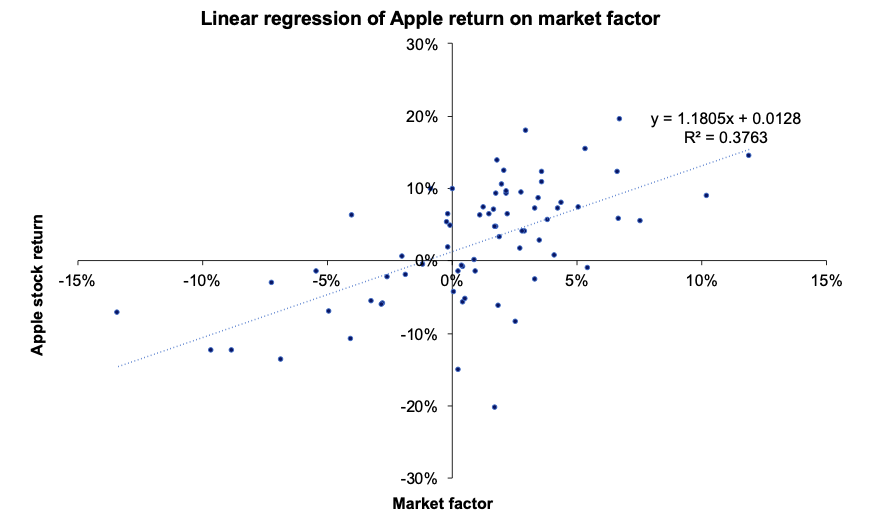
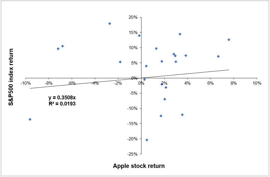
Figure 1 represents for a given asset (Apple stocks) the regression of its return with respect to the S&P500 index return (representing the market factor in the CAPM). The slope of the regression line corresponds to the beta of the regression equation.

Figure 1. Step 1: time-series regression for a given asset (Apple stock and the S&P500 index).
Source: computation by the author.

Step 2: cross-sectional analysis of returns

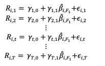
For each period t (from t equal 1 to T), we estimate the following cross-section linear regression model:

Fama MacBeth cross-section regression

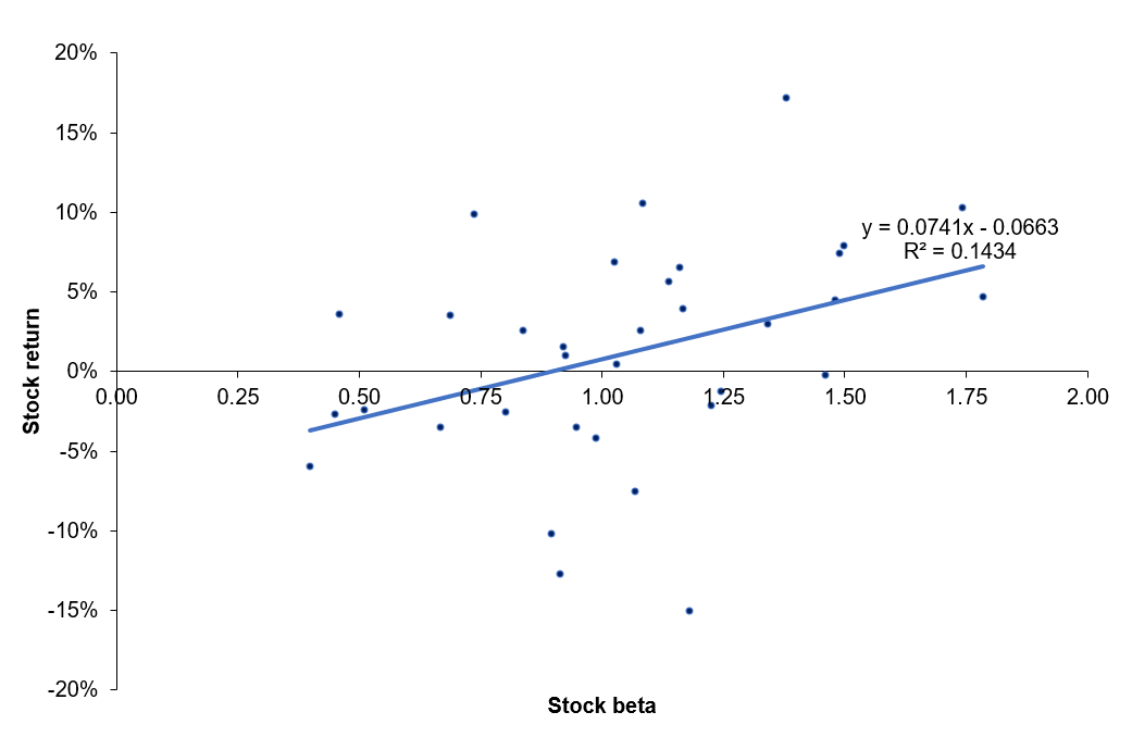
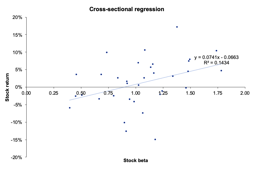
Figure 2 plots for a given period the cross-sectional returns and betas for a given point in time.

Figure 2 represents for a given period the regression of the return of all individual assets with respect to their estimated individual market beta.

Figure 2. Step 2: cross-section regression for a given time-period.

Source: computation by the author.

We average the gamma obtained for each data point. This is the way the Fama-MacBeth method is used to test asset pricing models.

Empirical study of the Fama-MacBeth regression

The seminal paper by Fama and MacBeth (1973) was based on an analysis of the market factor by assessing constructed portfolios of similar betas ranked by increasing values. This approach helped to overcome the shortcoming regarding the stability of the beta and correct for conditional heteroscedasticity derived from the computation of the betas for individual stocks. They performed a second time the cross-sectional regression of monthly portfolio returns based on equity betas to account for the dynamic nature of stock returns, which help to compute a robust standard error and assess if there is any heteroscedasticity in the regression. The conclusion of the seminal paper suggests that the beta is “dead”, in the sense that it cannot explain returns on its own (Fama and MacBeth, 1973).

Empirical study: Stock approach

We downloaded a sample of end-of-month stock prices of large firms in the US economy over the period from March 31, 2016, to March 31, 2022. We computed monthly returns. To represent the market, we chose the S&P500 index.

We then applied the Fama-MacBeth two-step regression method to test the market factor (CAPM).

Figure 3 depicts the computation of average returns and the betas and stock in the analysis.

Figure 3. Computation of average returns and betas of the stocks.
Source: computation by the author.

Figure 4 represents the first step of the Fama-MacBeth regression. We regress the average returns for each stock with their respective betas.

Figure 4. Step 1 of the regression: Time-series analysis of returns
Source: computation by the author.

The initial regression is statistically evaluated. To describe the behavior of the regression, we employ a t-statistic. Since the p-value is in the rejection area (less than the significance limit of 5 percent), we can deduce that the market factor can at first explain the returns of an investor. However, as we are going deal in the later in the article, when we account for a second regression as formulated by Fama and MacBeth (1973), the market factor is not capable of explaining on its own the return of asset returns.

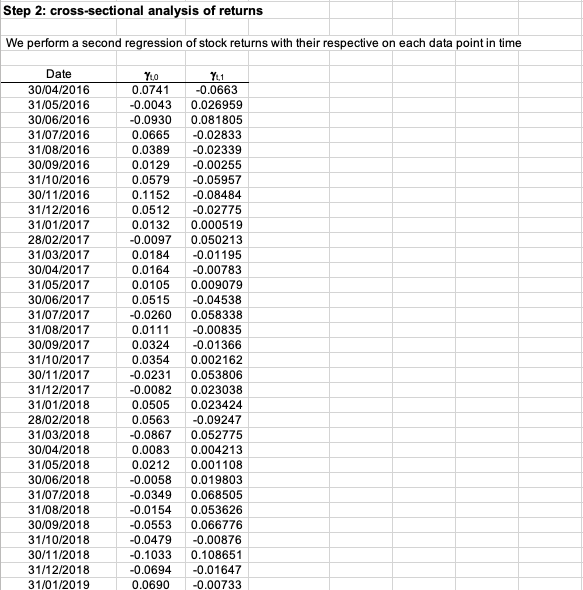
Figure 5 represents Step 2 of the Fama-MacBeth regression, where we perform for a given data point a regression of all individual stock returns with their respective estimated market beta.

Figure 5. Step 2: cross-sectional analysis of return.
Source: computation by the author.

Figure 6 represents the hypothesis testing for the cross-sectional regression. From the results obtained, we can clearly see that the p-value is not in the rejection area (at a 5% significance level), hence we cannot reject the null hypothesis. This means that the market factor fails to explain properly the behavior of asset returns, which undermines the validity of the CAPM framework. These results are in line with Fama-MacBeth (1973).

Figure 6. Hypothesis testing of the cross-sectional regression.
Source: computation by the author.

Excel file for the Fama-MacBeth two-step regression method

You can find below the Excel spreadsheet that complements the explanations covered in this article to implement the Fama-MacBeth two-step regression method.

Limitations of the Fama-McBeth approach

Selection of the market index

For the CAPM to be valid, we need to determine if the market portfolio is in the Markowitz efficient curve. According to Roll (1977), the market portfolio is not observable because it cannot capture all the asset classes (human capital, art, and real estate among others). He then believes that the returns cannot be captured effectively and hence makes the market portfolio, not a reliable factor in determining its efficiency.

Furthermore, the coefficients estimated in the time-series regressions are sensitive to the market index chosen for the study. These shortcomings must be taken into account when assessing CAPM studies.

Stability of the coefficients

The beta of individual assets are not stable over time. Fama and MacBeth attempted to address this shortcoming by implementing an innovative approach.

When betas are computed using a monthly time-series, the statistical noise of the time series is considerably reduced as opposed to shorter time frames (i.e., daily observation).

Using portfolio betas makes the coefficient much more stable than using individual betas. This is due to the diversification effect that a portfolio can achieve, reducing considerably the amount of specific risk.

Conclusion

Why should I be interested in this post?

Useful resources

Academic research

Brooks, C., 2019. Introductory Econometrics for Finance (4th ed.). Cambridge: Cambridge University Press. doi:10.1017/9781108524872

Fama, E. F., MacBeth, J. D., 1973. Risk, Return, and Equilibrium: Empirical Tests. Journal of Political Economy, 81(3), 607–636.

Roll R., 1977. A critique of the Asset Pricing Theory’s test, Part I: On Past and Potential Testability of the Theory. Journal of Financial Economics, 1, 129-176.

American Finance Association & Journal of Finance (2008) Masters of Finance: Eugene Fama (YouTube video)

Business Analysis

NEDL. 2022. Fama-MacBeth regression explained: calculating risk premia (Excel). [online] Available at: [Accessed 29 May 2022].

About the author

The article was written in December 2022 by Youssef LOURAOUI (Bayes Business School, MSc. Energy, Trade & Finance, 2021-2022).

Fama-MacBeth two-step regression method

January 30, 2024July 2, 2022 by Youssef LOURAOUI

In this article, Youssef Louraoui (Bayes Business School, MSc. Energy, Trade & Finance, 2021-2022) presents the Fama-MacBeth two-step regression method used to test asset pricing models.

This article is structured as follow: we introduce the Fama-MacBeth testing method. Then, we present the mathematical foundation that underpins their approach. We conclude with a practical case study followed by a discussion on econometric issues.

Introduction

Risk factors are frequently employed to explain asset returns in asset pricing theories. These risk factors may be macroeconomic (such as consumer inflation or unemployment) or microeconomic (such as firm size or various accounting and financial metrics of the firms). The Fama-MacBeth two-step regression approach a practical way for measuring how correctly these risk factors explain asset or portfolio returns. The aim of the model is to determine the risk premium associated with the exposure to these risk factors.

Mathematical foundations

We describe below the mathematical foundations for the Fama-MacBeth two-step regression method.

Step 1: time-series analysis of returns

The model considers the following inputs:

The return of N assets denoted by R_i for asset i observed over the time period [0, T].
The risk factors denoted by F₁ for the market factor influencing the asset returns.

For each asset i from 1 to N, we estimate the following parameters:

From this model, we obtain a series of coefficients: α_i which is the risk premium for asset i and the β_{i, F₁ associated to the market risk factor.}

Figure 1 represents for a given asset the regression of a return with respect to the market factor (as in the CAPM). The slope of the regression line corresponds to the market beta of the regression.

Figure 1 Time-series regression.
Source : computation by the author.

The econometric issues (estimation bias, heteroscedasticity, and autocorrelation) related to the model are discussed in more details in the econometric limitation section.

Step 2: cross-sectional analysis of returns

For each period t from 1 to T, we estimate the following linear regression model:

Figure 2 plots for a given period the cross-sectional returns and betas for a given point in time.

Figure 2 represents for a given period the regression of the return of all individual assets with respect to their estimated individual market beta.

Figure 2. Cross-sectional regression.
Time-series regression Source: computation by the author.

We average the gamma obtained for each data point. This is the way the Fama-MacBeth method is used to test asset pricing models.

Empirical study by Fama and MacBeth (1973)

Fama-MacBeth performed a second time the cross-sectional regression of monthly stock returns on the equity betas computed on the initial workings to account for the dynamic nature of stock returns, which help to compute a robust standard error to gauge the level of error and assess if there is any heteroscedasticity in the regression. The conclusion of the seminal paper suggests that the beta is “dead”, in the sense that it cannot explain returns on its own (Fama and MacBeth, 1973).

New empirical study

We then applied the Fama-MacBeth two-step regression method to test the market factor (CAPM).

Figure 3 depicts the computation of average returns and the betas and stock in the analysis.

Figure 3. Computation of average returns and betas of the stocks.
Source: computation by the author.

Figure 4 represents the first step of the Fama-MacBeth regression. We regress the average returns for each stock with their respective betas.

Figure 4. Step 1 of the regression: Time-series analysis of returns
Source: computation by the author.

The initial regression is statistically evaluated. To describe the behaviour of the regression, we employ a t-statistic. Since the p-value is in the rejection area (less than the significance limit of 5 percent), we can deduce that the market factor can at first explain the returns of an investor. However, as we are going deal in the later in the article, when we account for a second regression as formulated by Fama and MacBeth, the market factor is not capable of explaining on its own the return of asset returns.

Figure 5 represents Step 2 of the Fama-MacBeth regression, where we perform for a given data point a regression of all individual stock returns with their respective estimated market beta.

Figure 5. Step 2: cross-sectional analysis of return.
Source : computation by the author.

Figure 6 represents the hypothesis testing for the cross-sectional regression. From the results obtained, we can clearly see that the p-value is not in the rejection area (at a 5% significance level), hence we cannot reject the null hypothesis. This means that the market factor fails to explain properly the behaviour of asset returns, which undermines the validity of the CAPM framework. These results are in line with the Fama-MacBeth paper (1973).

Figure 6. Hypothesis testing of the cross-sectional regression.
Source: computation by the author.

Excel file for the Fama-MacBeth two-step regression method

You can find below the Excel spreadsheet that complements the explanations covered in this article to apply the Fama-MacBeth two-step regression method.

Econometric issues

Errors in data measurement

Because regression uses a sample instead of the entire population, a certain margin of error must be accounted for since the authors derive estimated betas for the sample.

Asset return heteroscedasticity

Asset return autocorrelation

Limitation of CAPM

Roll: selection of the appropriate market index

Furthermore, the coefficients are sensitive to the market index chosen for the study. These shortcomings must be taken into account when assessing other CAPM studies.

Fama-MacBeth: Stability of the coefficients

The stability of the beta across time is difficult. Fama-MacBeth attempted to address this shortcoming by implementing its innovative approach. However, some points need to be addressed:

When betas are computed using a monthly time series, the statistical noise of the time series is considerably reduced as opposed to shorter time frames (i.e., daily observation).

Constructing portfolio betas makes the coefficient much more stable than when assessing individual betas. This is due to the diversification effect that a portfolio can achieve, reducing considerably the amount of specific risk.

Why should I be interested in this post?

Useful resources

Academic research

Brooks, C., 2019. Introductory Econometrics for Finance (4th ed.). Cambridge: Cambridge University Press. doi:10.1017/9781108524872

Fama, E. F., MacBeth, J. D., 1973. Risk, Return, and Equilibrium: Empirical Tests. Journal of Political Economy, 81(3), 607–636.

Roll R., 1977. A critique of the Asset Pricing Theory’s test, Part I: On Past and Potential Testability of the Theory. Journal of Financial Economics, 1, 129-176.

American Finance Association & Journal of Finance (2008) Masters of Finance: Eugene Fama (YouTube video)

Business Analysis

NEDL. 2022. Fama-MacBeth regression explained: calculating risk premia (Excel). [online] Available at: [Accessed 29 May 2022].

About the author

The article was written in May 2022 by Youssef LOURAOUI (Bayes Business School, MSc. Energy, Trade & Finance, 2021-2022).

Specific risk

April 1, 2022 by Youssef LOURAOUI

In this article, Youssef LOURAOUI (Bayes Business School, MSc. Energy, Trade & Finance, 2021-2022) explains the specific risk of financial assets, a key concept in asset pricing models and asset management in practice.

This article is structured as follows: we start with a reminder of portfolio theory and the central concept of risk in financial markets. We then introduce the concept of specific risk of an individual asset and especially its sources. We then detail the mathematical foundation of risk. We finish with an insight of the relationship between diversification and risk reduction with a practical example to test this concept.

Portfolio Theory and Risk

Markowitz (1952) and Sharpe (1964) created a framework for risk analysis based on their seminal contributions to portfolio theory and capital market theory. All rational profit-maximizing investors attempt to accumulate a diversified portfolio of risky assets and borrow or lend to achieve a risk level consistent with their risk preferences given a set of assumptions. They established that the key risk indicator for an individual asset in these circumstances is its correlation with the market portfolio (the beta).

The variance of returns of an individual asset can be decomposed as the sum of systematic risk and specific risk. Systematic risk refers to the proportion of the asset return variance that can be attributed to the variability of the whole market. Specific risk refers to the proportion of the asset return variance that is unconnected to the market and reflects the unique nature of the asset. Specific risk is often regarded as insignificant or irrelevant because it can be eliminated in a well-diversified portfolio.

Sources of specific risk

Specific risk can find its origin in business risk (in the assets side of the balance sheet) and financial risk (in the liabilities side of the balance sheet):

Business risk

Internal or external issues might jeopardize a business. Internal risk is directly proportional to a business’s operational efficiency. An internal risk would include management neglecting to patent a new product, so eroding the company’s competitive advantage.

Financial risk

This pertains to the capital structure of a business. To continue growing and meeting financial obligations, a business must maintain an ideal debt-to-equity ratio.

Mathematical foundations

Following the Capital Asset Pricing Model (CAPM), the return on asset i, denoted by R_i can be decomposed as

img_SimTrade_return_decomposition

Where:

R_i the return of asset i
E(R_i) the risk premium of asset i
β_i the measure of the risk of asset i
R_M the return of the market
E(R_M) the risk premium of the market
R_M – E(R_M) the market factor
ε_i represent the specific part of the return of asset i

The three components of the decomposition are the expected return, the market factor and an idiosyncratic component related to asset only. As the expected return is known over the period, there are only two sources of risk: systematic risk (related to the market factor) and specific risk (related to the idiosyncratic component).

The beta of the asset with the market is computed as:

Beta

Where:

σ_i,m : the covariance of the asset return with the market return
σ_m² : the variance of market return

The total risk of the asset measured by the variance of asset returns can be computed as:

Decomposition of total risk

Where:

β_i² * σ_m² = systematic risk
σ_εi² = specific risk

In this decomposition of the total variance, the first component corresponds to the systematic risk and the second component to the specific risk.

Decomposition of returns

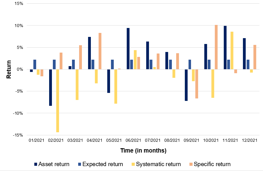
We analyze the decomposition of returns on Apple stocks. Figure 1 gives for every month of 2021 the decomposition of Apple stock returns into three parts: expected return, market factor (systematic return) and an idiosyncratic component (specific return). We used historical price downloaded from the Bloomberg terminal for the period 1999-2022.

Figure 1. Decomposition of Apple stock returns:
expected return, systematic return and specific return.
Decomposition of asset returns Computation by the author (data: Bloomberg).

You can download below the Excel file which illustrates the decomposition of returns on Apple stocks.

Why should I be interested in this post?

Investors will be less influenced by single incidents if they possess a range of firm stocks across several industries, as well as other types of assets in a number of asset classes, such as bonds and stocks.

An investor who only bought telecommunication equities, for example, would be exposed to a high amount of unsystematic risk (also known as idiosyncratic risk). A concentrated portfolio can have an impact on its performance. This investor would spread out telecommunication-specific risks by adding uncorrelated positions to their portfolio, such as firms outside of the telecommunication market.

Useful resources

Academic research

Evans, J.L., Archer, S.H. 1968. Diversification and the Reduction of Dispersion: An Empirical Analysis. The Journal of Finance, 23(5): 761–767.

Markowitz, H. 1952. Portfolio Selection. The Journal of Finance, 7(1): 77-91.

Mossin, J. 1966. Equilibrium in a Capital Asset Market. Econometrica, 34(4): 768-783.

Sharpe, W.F. 1963. A Simplified Model for Portfolio Analysis. Management Science, 9(2): 277-293.

Sharpe, W.F. 1964. Capital Asset Prices: A Theory of Market Equilibrium under Conditions of Risk. The Journal of Finance, 19(3): 425-442.

Tole T.M. 1982. You can’t diversify without diversifying. The Journal of Portfolio Management. Jan 1982, 8 (2) 5-11.

About the author

The article was written in April 2022 by Youssef LOURAOUI (Bayes Business School, MSc. Energy, Trade & Finance, 2021-2022).

Systematic risk

April 1, 2022 by Youssef LOURAOUI

In this article, Youssef LOURAOUI (Bayes Business School, MSc. Energy, Trade & Finance, 2021-2022) presents the systematic risk of financial assets, a key concept in asset pricing models and investment management theories more generally.

This article is structured as follows: we introduce the concept of systematic risk. We then explain the mathematical foundation of this concept. We present an economic understanding of market risk on recent events.

Portfolio Theory and Risk

Markowitz (1952) and Sharpe (1964) developed a framework on risk based on their significant work in portfolio theory and capital market theory. All rational profit-maximizing investors seek to possess a diversified portfolio of risky assets, and they borrow or lend to get to a risk level that is compatible with their risk preferences under a set of assumptions. They demonstrated that the key risk measure for an individual asset is its covariance with the market portfolio under these circumstances (the beta).

The fraction of an individual asset’s total variance attributable to the variability of the total market portfolio is referred to as systematic risk, which is assessed by the asset’s covariance with the market portfolio. Systematic risk can be decomposed into the following categories:

Interest rate risk

We are aware that central banks, such as the Federal Reserve, periodically adjust their policy rates in order to boost or decrease the rate of money in circulation in the economy. This has an effect on the interest rates in the economy. When the central bank reduces interest rates, the money supply expands, allowing companies to borrow more and expand, and when the policy rate is raised, the reverse occurs. Because this is cyclical in nature, it cannot be diversified.

Inflation risk

When inflation surpasses a predetermined level, the purchasing power of a particular quantity of money reduces. As a result of the fall in spending and consumption, overall market returns are reduced, resulting in a decline in investment.

Exchange Rate Risk

As the value of a currency reduces in comparison to other currencies, the value of the currency’s returns reduces as well. In such circumstances, all companies that conduct transactions in that currency lose money, and as a result, investors lose money as well.

Geopolitical Risks

When a country has significant geopolitical issues, the country’s companies are impacted. This can be mitigated by investing in multiple countries; but, if a country prohibits foreign investment and the domestic economy is threatened, the entire market of investable securities suffers losses.

Natural disasters

All companies in countries such as Japan that are prone to earthquakes and volcanic eruptions are at risk of such catastrophic calamities.

Following the Capital Asset Pricing Model (CAPM), the return on asset i, denoted by R_i can be decomposed as

img_SimTrade_return_decomposition

Where:

R_i the return of asset i
E(R_i) the risk premium of asset i
β_i the measure of the risk of asset i
R_M the return of the market
E(R_M) the risk premium of the market
R_M – E(R_M) the market factor
ε_i represent the specific part of the return of asset i

The beta of the asset with the market is computed as:

Beta

Where:

σ_i,m : the covariance of the asset return with the market return
σ_m² : the variance of market return

The total risk of the asset measured by the variance of asset returns can be computed as:

Decomposition of total risk

Where:

β_i² * σ_m² = systematic risk
σ_εi² = specific risk

In this decomposition of the total variance, the first component corresponds to the systematic risk and the second component to the specific risk.

Systematic risk analysis in recent times

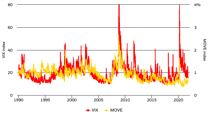
The volatility chart depicts the evolution of implied volatility for the S&P 500 and US Treasury bonds – the VIX and MOVE indexes, respectively. Implied volatility is the price of future volatility in the option market. Historically, the two markets have been correlated during times of systemic risk, like as in 2008 (Figure 1).

Figure 1. Volatility trough time (VIX and MOVE index).

Sources: BlackRock Risk and Quantitative Analysis and BlackRock Investment Institute, with data from Bloomberg and Bank of America Merrill Lynch, October 2021 (BlackRock, 2021).

The VIX index has declined following a spike in September amid the equity market sell-off. It has begun to gradually revert to pre-Covid levels. The periodic, albeit brief, surges throughout the year underscore the underlying fear about what lies beyond the economic recovery and the possibility of a wide variety of outcomes. The MOVE index — a gauge of bond market volatility – has remained relatively stable in recent weeks, despite the rise in US Treasury yields to combat the important monetary policy to combat the effect of the pandemic. This could be a reflection of how central banks’ purchases of government bonds are assisting in containing interest rate volatility and so supporting risk assets (BlackRock, 2021).

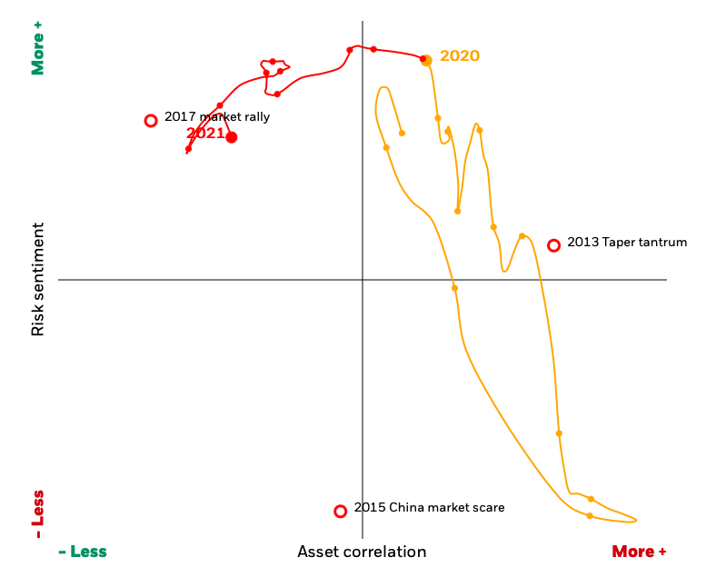
The regime map depicts the market risk environment in two dimensions by plotting market risk sentiment and the strength of asset correlations (Figure 2).

Figure 2. Regime map for market risk environment.

Source: BlackRock Risk and Quantitative Analysis and BlackRock Investment Institute, October 2021 (BlackRock, 2021).

Positive risk sentiment means that riskier assets, such as equities, are outperforming less risky ones. Negative risk sentiment means that higher-risk assets underperform lower-risk assets.

Due to the risk of fast changes in short-term asset correlations, investors may find it challenging to guarantee their portfolios are correctly positioned for the near future. When asset correlation is higher (as indicated by the right side of the regime map), diversification becomes more difficult and risk increases. When asset prices are less correlated (on the left side of the map), investors have greater diversification choices.

When both series – risk sentiment and asset correlation – are steady on the map, projecting risk and return becomes easier. However, when market conditions are unpredictable, forecasting risk and return becomes substantially more difficult. The map indicates that we are still in a low-correlation environment with a high-risk sentiment, which means that investors are rewarded for taking a risk (BlackRock, 2021). In essence, investors should use diversification to reduce the specific risk of their holding coupled with macroeconomic fundamental analysis to capture the global dynamics of the market and better understand the sources of risk.

Why should I be interested in this post?

Market risks fluctuate throughout time, sometimes gradually, but also in some circumstances dramatically. These adjustments typically have a significant impact on the right positioning of a variety of different types of investment portfolios. Investors must walk a fine line between taking enough risks to achieve their objectives and having the proper instruments in place to manage sharp reversals in risk sentiment.

Useful resources

Academic research

Markowitz, H. 1952. Portfolio Selection. The Journal of Finance, 7(1): 77-91.

Mossin, J. 1966. Equilibrium in a Capital Asset Market. Econometrica, 34(4): 768-783.

Sharpe, W.F. 1963. A Simplified Model for Portfolio Analysis. Management Science, 9(2): 277-293.

Sharpe, W.F. 1964. Capital Asset Prices: A Theory of Market Equilibrium under Conditions of Risk. The Journal of Finance, 19(3): 425-442.

Business analysis

BlackRock, 2021. Market risk monitor

About the author

The article was written in April 2022 by Youssef LOURAOUI (Bayes Business School, MSc. Energy, Trade & Finance, 2021-2022).

Monte Carlo simulation method

March 17, 2022 by Jayati WALIA

In this article, Jayati WALIA (ESSEC Business School, Grande Ecole – Master in Management, 2019-2022) explains the Monte Carlo simulation method and its applications in finance.

Introduction

Monte Carlo simulations are a broad class of computational algorithms that rely majorly on repeated random sampling to obtain numerical results. The underlying concept is to model the multiple possible outcomes of an uncertain event. It is a technique used to understand the impact of risk and uncertainty in prediction and forecasting models.

The Monte Carlo method was invented by John von Neumann (Hungarian-American mathematician and computer scientist) and Stanislaw Ulam (Polish mathematician) during World War II to improve decision making under uncertain conditions. It is named after the popular gambling destination Monte Carlo, located in Monaco and home to many famous casinos. This is because the random outcomes in the Monte Carlo modeling technique can be compared to games like roulette, dice and slot machines. In his autobiography, ‘Adventures of a Mathematician’, Ulam mentions that the method was named in honor of his uncle, who was a gambler.

How Monte Carlo simulation works

The main idea is to repeatedly run a large number of simulations of a random process for a variable of interest (such as an asset price in finance) covering a wide range of possible situations. The outcomes of this variables are drawn from a pre-specified probability distribution that is assumed to be known, including the analytical function and its parameters. Thus, Monte Carlo simulations inherently try to recreate the entire distribution of asset prices.

Example: Apple stock

Consider the Apple stock as our asset of interest for which we will generate stock prices according to the Monte Carlo simulation method.

The first step in the simulation is choosing a stochastic model for the behavior of our random variable (the Apple stock price in our case). A commonly used model is the geometric Brownian motion (GBM) model. The model assumes that future asset price changes are uncorrelated over time and the probability distribution function of the future price is a log-normal distribution. The movements in price in GBM process can be expressed as:

img_SimTrade_GBM_process

with dS being the change in asset price in continuous time dt. dW is the Wiener process (W_t+1 – W_t is a random variable from the normal distribution N(0, 1)). σ represents the price volatility considering the unexpected changes that can result from external effects (σ is assumed to be constant over time). μdt together represents the deterministic return within the time interval with μ representing the growth rate of the asset price or the ‘drift’.

Integrating dS/S over a finite interval, we get :

img_SimTrade_simulated_asset_price

Where ε is a random number generated from a normal distribution N(0,1).

This equation thus gives us the evolution of the asset price from a simulated model from day t-1 to day t.

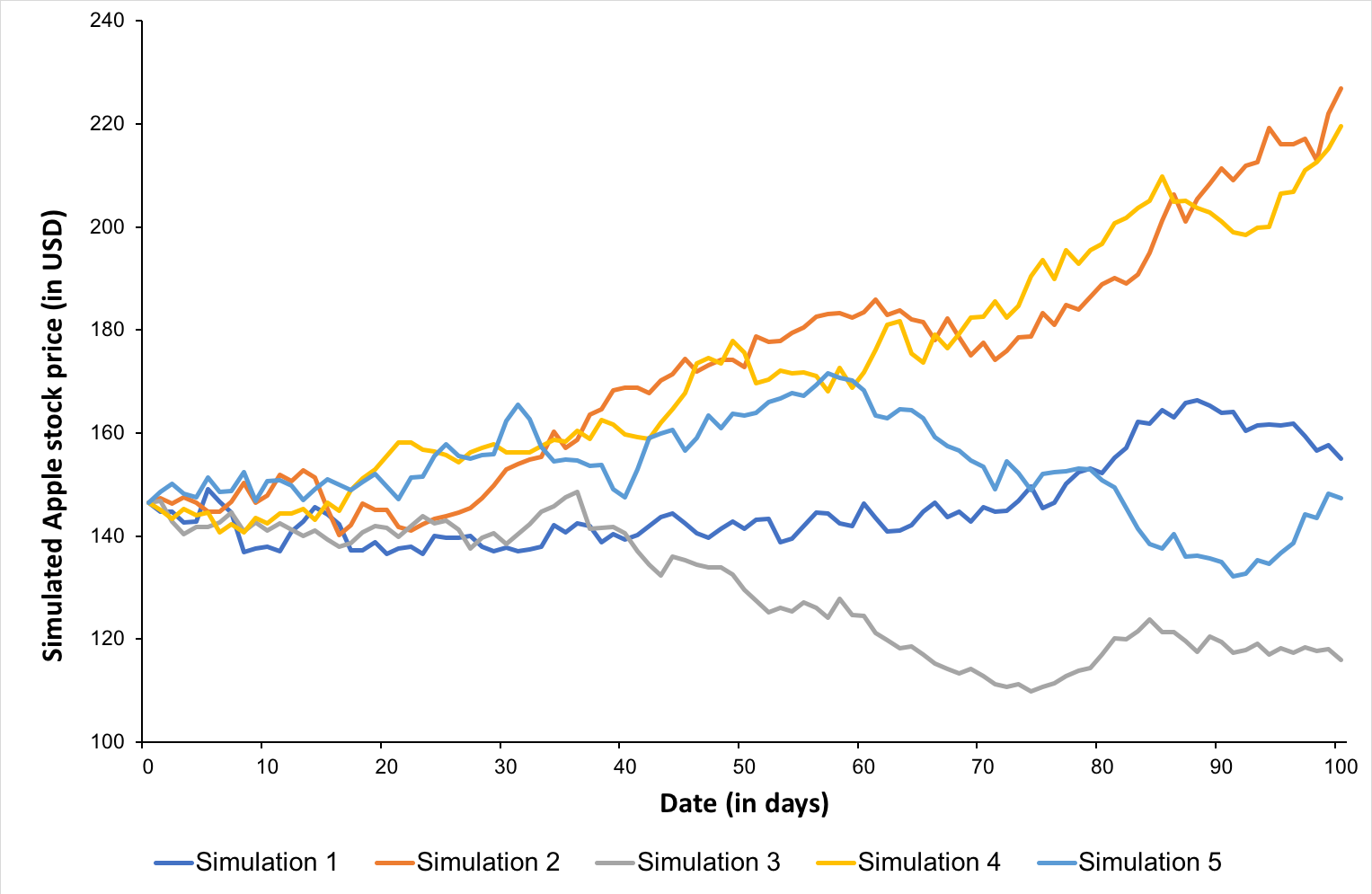
We can now generate a simulation path for 100 days using the above formula.

The figure below shows five simulations for the price of the Apple stock over 100 days with Δt = 1 day. The initial price for Apple stock (i.e, price at t=0) is $146.52.

Figure 1. Simulated Apple stock prices according to the Monte Carlo simulation method.
img_SimTrade_Apple_MonteCarloSim
Source: computation by author.

Thus, we can observe that the prices obtained by just these five simulations range from $100 to over $220.

You can download below the Excel file for generating Monte Carlo Simulations for Apple stock.

Applications in finance

The Monte Carlo simulation method is widely used in finance for valuation and risk analysis purposes.

One popular application is option pricing. For option contracts with complicated features (such as Asian options) or those with a combination of assets as their underlying, Monte Carlo simulations help generate multiple potential payoff scenarios for the option which are averaged out to determine the option price at the issuance date.

The Monte Carlo method is also used to assess potential risks by generating simulations of market variables affecting portfolios such as asset returns, interest rates, macroeconomic factors, etc. over different time periods. These simulations are then assessed as required for risk modelling and to compute risk metrics such as the value at Risk (VaR) of a position.

Other applications include personal finance planning and corporate project finance where simulations are generated to construct stochastic financial models for sensitivity analysis and net present value (NPV) projections.

Useful resources

Hull, J.(2008) Risk Management and Financial Institutions, Fifth Edition, Chapter 7 – Valuation and Scenario Analysis.

About the author

The article was written in March 2022 by Jayati WALIA (ESSEC Business School, Grande Ecole Program – Master in Management, 2019-2022).

Beta

November 20, 2021 by Youssef LOURAOUI

In this article, Youssef LOURAOUI (Bayes Business School, MSc. Energy, Trade & Finance, 2021-2022) explains the concept of beta, one of the most fundamental concepts in the financial industry, which is heavily used in asset management to assess the risk of assets and portfolios.

This article is structured as follows: we introduce the concept of beta in asset management. Next, we present the mathematical foundations of the concept. We finish with an interpretation of beta values for risk analysis.

Introduction

The (market) beta represents the sensitivity of an individual asset or a portfolio to the fluctuations of the market. This risk measure helps investors to predict the movements of their assets according to the movements of the market overall. It measures the asset risk in comparison with the systematic risk inherent to the market.

In practice, the beta for a portfolio (fund) in respect to the market M represented by a predefined index (the S&P 500 index for example) indicates the fund’s sensitivity to the index. Essentially, the fund’s beta to the index attempts to capture the amount of money made (or lost) when the index increases (or decreases) by a specified amount.

Graphically, the beta represents the slope of the straight line through a regression of data points between the asset return in comparison to the market return for different time periods. It is a traditional risk measure used in the asset management industry. To give a more insightful explanation, a regression analysis has been performed using data for the Apple stock (APPL) and the S&P500 index to see how the stock behaves in relation to the market fluctuations (monthly data for the period July 2018 – June 2020). Figure 1 depicts the regression between Apple stock and the S&P500 index (excess) returns. The estimated beta is between zero and one (beta = 0.3508), which indicates that the stock price fluctuates less than the market index.

Figure 1. Linear regression of the Apple stock return on the S&P500 index return.

Source: Computation by the author (data source: Thomson Reuters).

Mathematical derivation of Beta

Use of beta

William Sharpe, John Lintner, and Jan Mossin separately developed key capital markets theory as a result of Markowitz’s previous works: the Capital Asset Pricing Model (CAPM). The CAPM was a huge evolutionary step forward in capital market equilibrium theory since it enabled investors to appropriately value assets in terms of systematic risk, defined as the market risk which cannot be neutralized by the effect of diversification.

The CAPM expresses the expected return of an asset a function of the risk-free rate, the beta of the asset, and the expected return of the market. The main result of the CAPM is a simple mathematical formula that links the expected return of an asset to these different components. For an asset i, it is given by:

CAPM risk beta relation

Where:

E(r_i) represents the expected return of asset i
r_f the risk-free rate
β_i the measure of the risk of asset i
E(r_m) the expected return of the market
E(r_m)- r_f the market risk premium.

The risk premium for asset i is equal to β_i(E(r_m)- r_f), that is the beta of asset i, β_i, multiplied by the risk premium for the market, E(r_m)- r_f.

In this model, the beta (β) parameter is a key parameter and is defined as:

CAPM beta formula

Where:

Cov(r_i, r_m) represents the covariance of the return of asset i with the return of the market
σ²(r_m) the variance of the return of the market.

Excel file to compute the beta

You can download below an Excel file with data for Apple stock returns and the S&P500 index returns (used as a representation of the market). This Excel file computes the beta of apple with the S&P500 index.

Interpretation of the beta

Beta helps investors to explain how the asset moves compared to the market. More specifically, we can consider the following cases for beta values:

β = 1 indicates a fluctuation between the asset and its benchmark, thus the asset tends to move at a similar rate than the market fluctuations. A passive ETF replicating an index will present a beta close to 1 with its associated index.
0 < β < 1 indicates that the asset moves at a slower rate than market fluctuations. Defensive stocks, stocks that deliver consistent returns without regarding the market state like P&G or Coca Cola in the US, tend to have a beta with the market lower than 1.
β > 1 indicates a more aggressive effect of amplification between the asset price movements with the market movements. Call options tend to have higher betas than their underlying asset.
β = 0 indicates that the asset or portfolio is uncorrelated to the market. Govies, or sovereign debt bonds, tend to have a beta-neutral exposure to the market.
β < 0 indicates an inverse effect of market fluctuation impact in the asset volatility. In this sense, the asset would behave inversely in terms of volatility compared to the market movements. Put options and Gold typically tend to have negative betas.

Why should I be interested in this post?

If you are a business school or university student, this post will help you to understand the fundamentals of investment.

Useful resources

Academic research

Fama, Eugene F. 1965. The Behavior of Stock Market Prices.Journal of Business 37: January 1965, 34-105.

Fama, Eugene F. 1967. Risk, Return, and General Equilibrium in a Stable Paretian Market. Chicago, IL: University of Chicago.Unpublished manuscript.

Fama, Eugene F. 1968. Risk, Return, and Equilibrium: Some Clarifying Comments. Journal of Finance, (23), 29-40.

Lintner, J. 1965a. The Valuation of Risk Assets and the Selection of Risky Investments in Stock Portfolios and Capital Budgets. The Review of Economics and Statistics 47(1): 13-37.

Lintner, J. 1965b. Security Prices, Risk and Maximal Gains from Diversification. The Journal of Finance 20(4): 587-615.

Mangram, M.E., 2013. A simplified perspective of the Markowitz Portfolio Theory. Global Journal of Business Research, 7(1): 59-70.

Markowitz, H., 1952. Portfolio Selection. The Journal of Finance, 7(1): 77-91.

Mossin, J. 1966. Equilibrium in a Capital Asset Market. Econometrica 34(4): 768-783.

Sharpe, W.F. 1963. A Simplified Model for Portfolio Analysis. Management Science 9(2): 277-293.

Sharpe, W.F. 1964. Capital Asset Prices: A Theory of Market Equilibrium under Conditions of Risk. The Journal of Finance 19(3): 425-442.

Business analysis

JP Morgan Asset Management, 2021. Glossary of investment terms: Beta

Man Institute, 2021. How to calculate the Beta of a portfolio to a factor

Nasdaq, 2021. Beta

About the author

The article was written in November 2021 by Youssef LOURAOUI (Bayes Business School, MSc. Energy, Trade & Finance, 2021-2022).

Capital Market Line (CML)

January 30, 2024November 20, 2021 by Youssef LOURAOUI

In this article, Youssef LOURAOUI (Bayes Business School, MSc. Energy, Trade & Finance, 2021-2022) presents the Capital Market Line (CML), a key concept in asset pricing derived from the Capital Asset Pricing Model (CAPM).

This article is structured as follows: we first introduce the concept. We then illustrate how to estimate the capital market line (CML). We finish by presenting the mathematical foundations of the CML.

Capital Market Line

An optimal portfolio is a set of assets that maximizes the trade-off between expected return and risk: for a given level of risk, the portfolio with the highest expected return, or for a given level of expected return, the portfolio with the lowest risk.

Let us consider two cases: 1) when investors have access to risky assets only; 2) when investors have access to risky assets and a risk-free asset (earning a constant interest rate, 2% for example below).

Risky assets

In the case of risky assets only, the efficient frontier (the set of optimal portfolios) is represented below in Figure 1.

Figure 1. Efficient frontier with risky assets only.
img_Simtrade_CML_graph_1
Source: Computation by the author.

Risky assets and a risk-free asset

In the case of risky assets and a risk-free asset, the efficient frontier (the set of optimal portfolios) is represented below in Figure 2. In this case, the efficient frontier is a straight line called the Capital Market Line (CML).

Figure 2. Efficient frontier with risky assets and a risk-free asset.

Source: Computation by the author.

The CML joins the risk-free asset and the tangency portfolio, which is the intersection with the efficient frontier with risky assets only. We can reasonably conclude from Figure 2 that, to increase expected return, an investor has to increase the amount of risk he or she takes to attain returns higher than the risk-free interest rate. As a result, the Sharpe ratio of the market portfolio equals the slope of the CML. If the Sharpe ratio is more than the CML, an investment strategy can be implemented, such as buying assets if the Sharpe ratio is greater than the CML and selling assets if the Sharpe ratio is less than the CML (Drake and Fabozzi, 2011).

Investors who allocate their money between a riskless asset and the risky market portfolio M can expect a return equal to the risk-free rate plus compensation for the number of risk units σ_P) they accept. This result is in line with the underlying notion of all investment theory: investors perform two services in the capital markets for which they might expect to be compensated. First, they enable someone else to utilize their money in exchange for a risk-free interest rate. Second, they face the risk of not receiving the promised returns in exchange for their invested capital. The term E(r_M)- R_f) / σ_M refers to the investor’s expected risk premium per unit of risk, which is also known as the expected compensation per unit of risk taken.

Figure 3 represents the Capital Market Line which connect the risk-free asset to the efficient frontier line. The straight line in Figure 3 represents a combination of a risky portfolio and a riskless asset. Any combination of the risk-free asset and Portfolio A is similarly outperformed by some combination of the risk-free asset and Portfolio B. Continue drawing a line from R_f to the efficient frontier with increasing slopes until you reach Portfolio M’s point of tangency. All other possible portfolio combinations that investors could build are outperformed by the collection of portfolio possibilities along Line R_f-M, which is the CML. The CML, in this sense, represents a new efficient frontier that combines the Markowitz efficient frontier of risky assets with the ability to invest in risk-free securities. The CML’s slope is (E(r_M)- R_f) / σ(_M), which is the highest risk premium compensation that investors can expect for each unit of risk they take on (Reilly and Brown, 2012) (Figure 3).

If we fully invest our cash on the risk-free rate, we would be exactly on the y axis with an expected return of 2%. Each time we move along the curve that connects the risk-free rate to the optimum market portfolio, we allocate less weight to the risk-free rate, and we overweight more on riskier assets (Point A). Points M represents the optimal risky portfolio in the efficient frontier line, which minimizes the overall portfolio variance. It would have a weighting of 45% in stock A and a 55% in stock B, which would offer a 26.23% annualized return for a 17.27% annualized volatility. Point B represents a portfolio composition that is based on a leveraged position of 140% on the optimal risky portfolio and a short position on the risk-free asset of -40% (Figure 3).

Figure 3. Efficient frontier with different points.

Source: Computation by the author.

Mathematical representation

We can define the CML as the line that is tangent to the efficient frontier which connects the risk-free asset with the market portfolio:

img_SimTrade_CML_equations_0

Where:

σ_P: the volatility of portfolio P
R_f: the risk-free interest rate
E(R_M): the expected return of the market M
σ_M: the volatility of the market M
E[R_M– R_f]: the market risk premium.

The expected return of the portfolio can be computed as:

img_SimTrade_CML_equations_1

The Sharpe Ratio is shown in parenthesis, and it compares the performance of an investment, such as a security or portfolio, to the performance of a risk-free asset after adjusting for risk. It is calculated by dividing the difference between the investment returns and the risk-free return by the standard deviation of the investment returns. It denotes the additional amount of return that an investor receives for each unit of risk increase (Sharpe, 1963). We can define it mathematically as:

img_SimTrade_CML_equations_2

We can identify the following relationship between the slope of the CML and the Sharpe ratio of the market portfolio, defined mathematically as follows:

img_SimTrade_CML_equations_3

A simple strategy for stock selection is to buy assets with Sharpe ratios that are higher than the CML and sell those with Sharpe ratios that are lower. Indeed, the efficient market hypothesis implies that beating the market is impossible. As a result, all portfolios should have a Sharpe ratio that is lower than or equal to the market. As a result, if a portfolio (or asset) has a higher Sharpe ratio than the market, this portfolio (or asset) has a higher return per unit of risk (i.e. volatility), which contradicts the efficient market hypothesis. The alpha is the abnormal excess return over the market return at a given level of risk.

Why should I be interested in this post?

Sharpe ratio is a popular tool for assessing portfolio risk/return in finance. The Sharpe ratio informs the investor precisely which portfolio has the best performance among the available options. This simplifies the investor’s decision-making process. The higher the ratio, the greater the return for each unit of risk.

If you are a business school or university undergraduate or graduate student, this content will help you in broadening your knowledge of finance.

Useful resources

Academic research

Pamela, D. and Fabozzi, F., 2010. The Basics of Finance: An Introduction to Financial Markets, Business Finance, and Portfolio Management. John Wiley and Sons Edition.

Lintner, J. 1965a. The Valuation of Risk Assets and the Selection of Risky Investments in Stock Portfolios and Capital Budgets. The Review of Economics and Statistics 47(1): 13-37.

Lintner, J. 1965b. Security Prices, Risk and Maximal Gains from Diversification. The Journal of Finance, 20(4): 587-615.

Mossin, J. 1966. Equilibrium in a Capital Asset Market. Econometrica, 34(4): 768-783.

Reilly, R. K., Brown C. K., 2012. Investment Analysis & Portfolio Management, Tenth Edition.

Sharpe, W.F. 1963. A Simplified Model for Portfolio Analysis. Management Science, 9(2): 277-293.

Sharpe, W.F. 1964. Capital Asset Prices: A Theory of Market Equilibrium under Conditions of Risk. The Journal of Finance, 19(3): 425-442.

About the author

The article was written in November 2021 by Youssef LOURAOUI (Bayes Business School, MSc. Energy, Trade & Finance, 2021-2022).

Origin of factor investing

September 12, 2021 by Youssef LOURAOUI

Origin of factor investing

In this article, Youssef LOURAOUI (ESSEC Business School, Global Bachelor of Business Administration, 2017-2021) presents the origin of factor investing. A factor is defined as a persistent driver that helps explain assets’ long-term risk and return properties across asset classes.

This article is structured as follows: we begin by presenting Markowitz’s Modern Portfolio Theory (MPT) as the origin of factor investing (market factor). We then explain the Fama-French three-factor models, which is an extension of the CAPM single factor model (market factor). Furthermore, we explain also the Carhart four-factor model and the Fama-French five-factor model that aimed to capture additional factors to the market factor.

Markowitz’s Modern Portfolio Theory: Origin of the factor investing

Factor investing can be retraced to the work of Harry Markowitz in the early 1950s. The most important aspect of Markowitz’s approach was his fundamental finding that an asset’s risk and return should not be evaluated on its own, but rather on how it contributes to the entire risk and return of a portfolio. His dissertation, titled “Portfolio Selection”, was published in The Journal of Finance (1952). Nearly thirty years later, Markowitz shared the Nobel Prize for economics and corporate finance for his MPT contributions to both disciplines. The holy grail of Markowitz’s work is based on his calculation of the variance of a two-asset portfolio computed as follows:

Where:

w and (1-w) represents asset weights of assets A and B
σ² represents the variance of the assets and portfolio
cov(r_A,r_B) represents the covariance of assets A and B.

Capital Asset Pricing Model (CAPM)

William Sharpe, John Lintner, and Jan Mossin separately developed another key capital markets theory as a result of Markowitz’s previous works : the Capital Asset Pricing Model (CAPM). The CAPM was a huge evolutionary step forward in capital market equilibrium theory, since it enabled investors to appropriately value assets in terms of systematic risk, defined as the market risk which cannot be neutralized by the effect of diversification. In his derivation of the CAPM, Sharpe, Mossin and Litner made significant contributions to the concepts of the Efficient Frontier and Capital Market Line. Sharpe, Litner and Mossin seminal contributions would later earn him the Nobel Prize in Economics. The CAPM is based on a set of market structure and investor hypotheses:

There are no intermediaries
There are no limits (short selling is possible)
Supply and demand are in balance
There are no transaction costs
An investor’s portfolio value is maximized by maximizing the mean associated with projected returns while reducing risk variance
Investors have simultaneous access to information in order to implement their investment plans
Investors are seen as “rational” and “risk averse”.

Under this framework, the expected return of a given asset is related to its risk measured by the beta:

Where :

E(r) represents the expected return of the asset
r_f the risk-free rate
β a measure of the risk of the asset
E(r_m) the expected return of the market
E[r_m– r_f]represents the market risk premium.

In this model, the beta (β) parameter is a key parameter and is defined as:

Where:

Cov(r, r_m) represents the covariance of the asset with the market
σ²(r_m) is the variance of market return.

According to the CAPM formula, beta may be thought in mathematical terms as the slope of the regression between the asset return and the market return. Thus, beta quantifies the asset sensitivity to changes in the market return;
According to the beta formula, it may be understood as the risk that each dollar invested in an asset adds to the market portfolio. This is an economic explanation based on the observation that the market portfolio’s risk (measured by 〖σ(r_m)〗^2) is a weighted average of the covariance risks associated with the assets in the market portfolio, making beta a measure of the covariance risk associated with an asset in comparison to the variance of the market return.

Additionally, the CAPM makes a distinction between two forms of risk: systematic and specific risk. Systematic risk refers to the risk posed by the market’s basic structure, its participants, and any and all non-diversifiable elements such as monetary policy, political events, and natural disasters. By contrast, specific risk refers to the risk inherent in a particular asset and so is diversifiable. As a result, the CAPM solely captures systematic risk via the beta measure, with the market’s beta equal to one, lower-risk assets having a beta less than one, and higher-risk assets having a beta larger than one.

Finally, the CAPM’s central message is that when investors invest in a particular security/portfolio, they are rewarded twice: once via the time value of money impact (reflected in the risk-free component of the CAPM equation) and once via the effect of taking on more risk. However, the CAPM is not an empirically sound model, owing to an unnecessarily simplified set of assumptions and problems in establishing validating tests at the model’s first introduction (Fama and French, 2004). Thus, throughout time, the CAPM has been revised and modified to address not just its inadequacies but also to keep pace with financial and economic changes. Sharpe (1990), in his evaluation of the CAPM, cites various examples of revisions to his basic model proposed by other economists and financial experts.

The Fama-French three-factor model

Eugene Fama and Kenneth French created the Fama-French Three-Factor model in 1993 in response to the CAPM’s inadequacy. It contends that, in addition to the market risk component introduced by the CAPM, two more factors affect the returns on securities and portfolios: market capitalization (referred to as the “size” factor) and the book-to-market ratio (referred to as the “value” factor). According to Fama and French, the primary rationale for include these characteristics is because both size and book-to-market (BtM) ratios are related to the economic fundamentals of the business issuing the securities (Fama and French, 1993).

They continue by stating that:

Earnings and book-to-market ratios are inversely associated, with companies with low book-to-market ratios consistently reporting better earnings than those with high book-to-market ratios
Due to a similar risk component, size and average returns are inversely associated. This is based on their observation of the trajectory of small business profits in the 1980s: they suggest that small enterprises experience longer durations of earnings depression than larger enterprises in the event of a recession in the economy in which they operate. Additionally, they noted that smaller enterprises did not contribute to the economic expansion in the mid- and late-1980s following the 1982 recession
Profitability is connected to both size and BtM, and is a common risk factor that emphasizes and explains the positive association between BtM ratios and average returns. As thus, the return on a security/portfolio becomes:

Where :

E(𝑟) is the expected return of the asset/portfolio
𝑟_𝑓 is the risk-free rate
𝛽 is the measure of the market risk of the asset
𝐸(𝑟_𝑀) is the expected return of the market
𝛽_𝑆 is the measure of the risk related to the size of the asset
𝛽_𝑉 is the measure of the risk related to the value of the security/portfolio
𝑆𝑀𝐵 (which stands for “Small Minus Big”) measures the difference in expected returns between small and big firms (in terms of market capitalization)
𝐻𝑀𝐿 (which stands for “High Minus Low”) measures the difference in expected returns between value stocks and growth stock
𝛼 is a regression intercept
𝜖 is a measure of regression error

Both SMB and HML are derived using historical data as well as a mixture of portfolios focused on size and value. Professor French publishes these values on a regular basis on his personal website. Meanwhile, the betas for both the size and value components are derived using linear regression and might be positive or negative. However, the Fama-French three-factor model is not without flaws. Griffin (2002) highlights a significant flaw in the model when he claims that the Fama-French components of value and size are more accurate at explaining return differences when applied locally rather than internationally. As a result, each of the components should be addressed on a nation-by-country basis (as professor French now does on his website, where he specifies the SMB and HML factors for each nation, such as the United Kingdom, France, and so on). While the Fama-French model has gone further than the CAPM in terms of breaking down security returns, it remains an incomplete model with spatially confined interpretation of its additional variables. Efforts have been made over the years to complete this model, with Fama and French adding two more variables in 2015, profitability and investment strategy, and other scholars, like as Carhart (1997), adding a fourth feature, momentum, to the original Three-Factor model.

The Carhart four-factor model

Carhart (1997) extended the Fama-French three-factor model (1993) by adding a fourth factor: momentum. Momentum is defined as the observable tendency for prices to continue climbing or declining following an initial increase or decline. By definition, momentum is an anomaly, as the Efficient Market Hypothesis (EMH) states that there is no reason for security prices to continue growing or declining after an initial change in their value.

While traditional financial theory is unable to define precisely what causes momentum in certain securities, behavioural finance provides some insight into why momentum exists; indeed, Chan, Jegadeesh and Lakonishok (1996) argue that momentum arises from the inability of the majority of investors to react quickly and immediately to new market information and, thus, integrate that information into securities. This argument demonstrates investors’ irrationality when it comes to appraising the value of certain stocks and making investing decisions. Carhart was motivated to incorporate the momentum component into the Fama-French three-factor model since the model was unable to account for return variance in momentum-sorted portfolios (Fama and French, 1996 – Carhart 1997). Carhart incorporated Jegadeesh and Titman’s (1993) one-year momentum variation into his model as a result.

Where the additional component represents:

𝛽_𝑀 is the measure of the risk related to the momentum factor of the security/portfolio
𝑈𝑀𝐷 (which stands for “Up Minus Down”) measures the difference in expected returns between “winning” securities and “losing” securities (in terms of momentum).

As Carhart states in his article, the four-factor model, like the CAPM and the Fama-French Three-Factor, may be used to explain the sources of return on a specific security/portfolio (Carhart, 1997).

The Fama-French five-factor model

Fama and French state in 2014 that the first three-factor model they developed in 1993 does not adequately account for certain observed inconsistencies in predicted returns. As a consequence, Fama and French enhanced the three-factor model by adding two new variables: profitability and investment. The justification for these two factors arises from the theoretical implications of the dividend discount model (DDM), which claims that profitability and investment help to explain the returns achieved from the HML element in the first model (Fama and French, 2015).

Surprisingly, unlike the Carhart model, the new Fama-French model does not incorporate the momentum element. This is mostly because to Fama’s position on momentum. While not denying its existence, Fama thinks that the degree of risk borne by securities in an efficient market cannot fluctuate so dramatically that it justifies the necessity to recognize the momentum factor’s involvement (Fama and French, 2015). According to the Fama-French five-factor model, the return on any security is calculated as follows:

𝛽_P is the measure of the risk related to the profitability factor of the security/portfolio
𝑅𝑀𝑊 (which stands for “Robust Minus Weak”) measures the difference in expected returns between securities that exhibit strong profitability levels (thus making them “robust”) and securities that show inconsistent profitability levels (thus making them “weak”)
𝛽_𝐼 is the measure of the risk related to the investment factor of the asset
𝐶𝑀𝐴 (which stands for “Conservative Minus Aggressive”) measures the difference in expected returns between securities that engage in limited investment activities (thus making them “conservative”) and securities that show high levels of investment activity (thus making them “aggressive”).

To validate the new model, Fama and French created many portfolios with considerable returns disparities due to size, value, profitability, and investing characteristics. Additionally, they completed two exercises:

The first is a regression of portfolio results versus the improved model. This was done to determine the extent to which it explains the observed returns disparities between the selected portfolios
The second is to compare the new model’s performance to that of the three-factor model. This was done to determine if the new five-factor model adequately accounts for the observed returns differences in the old three-factor model. The following summarizes Fama and French’s conclusions about the new model.

The HML component becomes superfluous in terms of structure, since any value contribution to a security’s return can already be accounted by market, size, investment, and profitability factors. Thus, Fama and French advise investors and scholars to disregard the HML effect if their primary objective is to explain extraordinary returns (Fama and French, 2015).

They do, however, argue for the inclusion of all five elements when attempting to explain portfolio returns that display size, value, profitability, and investment tilts. Additionally, the model explains between 69% and 93% of the return disparities seen following the usage of the prior three-factor model (Fama and French, 2015). This new model, however, is not without flaws. Blitz, Hanauer, Vidojevic, and van Vliet (henceforth referred to as BHVV) identified five problems with the new Fama-French five-factor model in their 2016 paper “Five difficulties with the Five-Factor model”.

While two of these issues are related to some of the original Fama-French three factor model’s original factors (most notably the continued existence within the model of the CAPM relationship between market risk and return, as well as the new model’s overall acceptance by the academic community while some of the original factors are still contested), several of the other issues are related to other factors. These concerns include the following (Fama and French, 2015) :

The lack of motion
The new factors introduced lack robustness. The questions here include historical (i.e., will these factors apply to data points before to 1963) and if these aspects also apply to other asset types
The absence of adequate empirical support for the implementation of these Fama and French components

Use of the asset pricing models

All the models presented above are mostly employed in asset management to analyze the performance of an actively managed portfolio and the overall performance of a mutual fund.

Why should I be interested in this post?

Useful resources

Academic research

Blitz, D., Hanauer M.X., Vidojevic M., van Vliet, P., 2018. Five Concerns with the Five-Factor Model, The Journal of Portfolio Management, 44(4): 71-78.

Carhart, M.M. (1997), On Persistence in Mutual Fund Performance. The Journal of Finance, 52: 57-82.

Fama, E.F., French, K.R., 1992. The Cross-Section of Expected Stock Returns. The Journal of Finance, 47: 427-465.

Fama, E.F., French, K.R., 2004. The Capital Asset Pricing Model: Theory and Evidence. Journal of Economic Perspectives, 18(3): 25-46.

Fama, E.F., French, K.R., 2015. A five-factor asset pricing model. Journal of Financial Economics, 116(1): 1-22.

Lintner, J. 1965a. The Valuation of Risk Assets and the Selection of Risky Investments in Stock Portfolios and Capital Budgets. The Review of Economics and Statistics 47(1): 13-37.

Lintner, J. 1965b. Security Prices, Risk and Maximal Gains from Diversification. The Journal of Finance 20(4): 587-615.

Mangram, M.E., 2013. A simplified perspective of the Markowitz Portfolio Theory. Global Journal of Business Research, 7(1): 59-70.

Markowitz, H., 1952. Portfolio Selection. The Journal of Finance, 7(1): 77-91.

Mossin, J. 1966. Equilibrium in a Capital Asset Market. Econometrica 34(4): 768-783.

Sharpe, W.F. 1963. A Simplified Model for Portfolio Analysis. Management Science 9(2): 277-293.

Sharpe, W.F. 1964. Capital Asset Prices: A theory of Market Equilibrium under Conditions of Risk. The Journal of Finance 19(3): 425-442.

About the author

The article was written in September 2021 by Youssef LOURAOUI (ESSEC Business School, Global Bachelor of Business Administration, 2017-2021).

Arbitrage Pricing Theory (APT)

Introduction

Assumptions of the APT model

Capital Asset Pricing Model (CAPM)

Mathematical foundations

Application

Applying APT

Excel file for the APT application

Why should I be interested in this post?

Related posts on the SimTrade blog

Useful resources

Academic research

Business Analysis

Time series

About the author

Fama-MacBeth two-step regression method: the case of K risk factors

Introduction

Mathematical foundations

Step 1: time-series analysis of returns

Step 2: cross-sectional analysis of returns

Application: the Fama-French 3-Factor model

Empirical study of the Fama-MacBeth regression

Empirical study: Stock approach for a K-factor model

Time-series regression

Cross-sectional regression

Excel file

Why should I be interested in this post?

Related posts on the SimTrade blog

Useful resources

Academic research

About the author

Fama-MacBeth regression method: the stock approach vs the portfolio approach

Introduction

Fama and MacBeth (1973) implemented with individual stocks

Step 1: time-series regression

Step 2: cross-sectional regression

Test the statistical significance of the results obtained from the regression

Fama and MacBeth (1973) implemented with portfolios of stocks

Step 1: time-series regression

Step 2: cross-sectional regression

Test the statistical significance of the results obtained from the regression

Econometric issues

Errors in data measurement

Asset return heteroscedasticity

Asset return autocorrelation

Why should I be interested in this post?

Related posts on the SimTrade blog

Useful resources

Academic research

About the author

Introduction

Mathematical foundations

Step 1: time-series analysis of returns

Step 2: cross-sectional analysis of returns

Empirical study of the Fama-MacBeth regression

Empirical study: Stock approach

Excel file for the Fama-MacBeth two-step regression method

Limitations of the Fama-McBeth approach

Selection of the market index

Stability of the coefficients

Conclusion

Why should I be interested in this post?

Related posts on the SimTrade blog

Useful resources

Academic research

Business Analysis

About the author

Introduction

Mathematical foundations

Step 1: time-series analysis of returns

Step 2: cross-sectional analysis of returns

Empirical study by Fama and MacBeth (1973)

New empirical study

Excel file for the Fama-MacBeth two-step regression method

Econometric issues

Errors in data measurement

Asset return heteroscedasticity

Asset return autocorrelation

Limitation of CAPM

Roll: selection of the appropriate market index