Extreme correlation

February 4, 2024January 31, 2024 by Shengyu ZHENG

Extreme correlation

In this article, Shengyu ZHENG (ESSEC Business School, Grande Ecole Program – Master in Management, 2020-2024) explains the concept of extreme correlation.

Background

In financial risk management, there is a concept that is often overlooked, the extreme correlation also known as tail dependence. Tail dependence reveals how extreme events in two variables are linked. The oversight could leave portfolios exposed to amplified risks during market turbulence. In this post, we will get to see the definition and implications of this concept.

Linear correlation and copula

As presented in the post on copula, using linear correlation to model the dependence structure between random variables poses many limitations, and copula is a more generalized tool that allows to capture a fuller picture of the dependence structure.

Let’s recall the definition of copula. A copula, denoted typically as C∶[0,1]^d→[0,1] , is a multivariate distribution function whose marginals are uniformly distributed on the unit interval. The parameter d is the number of variables. For a set of random variables U₁, …, U_d with cumulative distribution functions F₁, …, F_d, the copula function C satisfies:

C(F₁(u₁),…,F_d(u_d)) = ℙ(U₁≤u₁,…,U_d≤u_d)

Here we introduce Student t-copula as an example, which will also be used as an illustration in the part of extreme correlation.

Tail dependence coefficient

The tail dependence coefficient captures the dependence level of a bivariate distribution at its tails. Let’s denote X and Y as two continuous random variables with continuous distribution F and G respectively. The (upper) tail dependence coefficient between X and Y is defined as:

with the limit of λ_U∈[0,1]

We can conclude that the tail dependence coefficient between two continuous random variables is a copula property, and it remains invariant with strict increasing transformations of the two random variables.

If λ_U∈(0,1], X and Y are considered asymptotically dependent in their (upper) tail. If λ_U=0, X and Y are considered asymptotically independent in their (upper) tail.

It is important to note that the independent of X and Y implies that λ_U=0, but the converse is not necessarily true. λ_U describes only the dependence level at the tails.

Examples of extreme correlation

Longin and Solnik (2001) and Gkillas and Longin (2019) employ the logistic model for the dependence function of the Gumbel copula (also called the Gumbel-Hougaard copula) for Fréchet margins, as follows:

This model contains the special cases of asymptotic independence and total dependence. It is parsimonious, as we only need one parameter to model the bivariate dependence structure of exceedances, i.e., the dependence parameter α with 0<α≤1. The correlation of exceedances ρ (also called extreme correlation) can be computed from the dependence parameter α of the logistic model as follows: ρ= 1-α^2. The special cases where α is equal to 1 and α converges towards 0 correspond to asymptotic independence, in which ρ is equal to 0, and total dependence, in which ρ is equal to 1, respectively (Tiago de Oliveira, 1973).

Useful resources

Academic resources

Gkillas K. and F. Longin (2018) Is Bitcoin the new digital Gold?, Working paper, ESSEC Business School.

Longin F. (2016) Extreme events in finance: a handbook of extreme value theory and its applications Wiley Editions.

Longin F. and B. Solnik (2001) Extreme Correlation of International Equity Markets, The Journal of Finance, 56, 649-676.

Zeevi A. and R. Mashal (2002) Beyond Correlation: Extreme Co-Movements between Financial Assets. Available at SSRN: https://ssrn.com/abstract=317122

Other resources

Extreme Events in Finance

Rieder H. E. (2014) Extreme Value Theory: A primer (slides).

About the author

The article was written in January 2024 by Shengyu ZHENG (ESSEC Business School, Grande Ecole Program – Master in Management, 2020-2024).

Optimal threshold selection for the peak-over-threshold approach of extreme value theory

January 28, 2024January 27, 2024 by Shengyu ZHENG

Optimal threshold selection for the peak-over-threshold approach of extreme value theory

In this article, Shengyu ZHENG (ESSEC Business School, Grande Ecole Program – Master in Management, 2020-2024) explains the different methods used to select the threshold for the tails for the peak-over-threshold (POT) approach of extreme value theory (EVT).

The Peak-over-Threshold threshold approach

As we have seen in the previous post, Extreme Value Theory: the Block-Maxima approach and the Peak-Over-Threshold approach, there are two main paradigms to model the extreme behavior of a random variable (say asset returns in finance).

Amongst the two, the POT approach makes use of all data entries above a designated high threshold u. The threshold exceedances could be fitted into a generalized Pareto distribution (GPD):

Illustration of the POT approach

Threshold selection

Along with the POT approach arises the issue of threshold selection to define when the tail of the distribution starts. Estimating parameters for extreme value distributions becomes more stable when based on exceedances beyond an appropriate threshold. In the tail, the distribution may behave more consistently, leading to more reliable parameter estimates. This stability is crucial for making accurate predictions about extreme events.

An efficient method for the computation of an optimal threshold optimizes the trade-off between bias and inefficiency (Jansen and de Vries, 1991). As explained by Gkillas, Katsiampa, and Longin (2021): “on the one hand, a low threshold value induces an estimation bias, due to observations not belonging to the distribution tails considered as exceedances. On the other hand, a high threshold value leads to inefficient estimates with high standard errors, due to the reduced size of the estimation sample”.

Methods of optimal threshold selection

There are several methods to this issue. We explain in detail the methods based on the plot analysis and Monte Carlo simulations. We also briefly discuss other methods: bootstrapping techniques, bias reduction, etc.

Plot analysis

The most known plot for deriving the optimal threshold is the Hill plot.

The Hill estimator is commonly used to estimate the tail index of a generalised Pareto distribution and to estimate the optimal threshold. The tail index is a measure of the heaviness of the tails of a distribution. According to the statistical order X_(1:n), the Hill estimator for the tail index α=1/ξ is given by

with k being the highest statistical order.

The Hill plot is a graphical representation of the Hill estimators. In a Hill plot, the sample data is sorted in descending order, and the plot shows the logarithm of the sample quantiles against their corresponding order statistics. The slope of the line in the plot provides information about the tail behaviour of the distribution. What we are looking for here is the point from where the plot starts to stabilise.

Here we have an example of a Hill Plot of the logarithmic losses of the S&P 500 index.

There exist alternative plots based on the standard Hill plot, such as Alternative Hill plot, smoothed Hill plot. These two alternatives are available in the evmix R package.

Monte Carlo simulations

Jansen and de Vries (1991) proposed a Monte Carlo simulation method as follows. Imagine we would like to study the behaviour of a random variable at its extreme. First a family of specific models for this random variable is assumed (say the family of Student-t distributions). Based on the assumption of a specific distribution, Monte Carlo simulations are launched. For each simulation, the optimal number of return exceedances is computed, and this corresponds to the optimal threshold. The mean squared error (MSE) of simulated optimal numbers of return exceedances is then calculated. With this result, we can derive the optimal threshold for the observed series. As Theil (1971) explains, the MSE criterion takes into account of a double effect of bias and inefficiency. The MSE of S simulated observations of the estimator of a parameter X could be represented as:

Where X̄ represents the mean of S simulated observations. The first part on the right of the equation represents the bias, and the second part represents the inefficiency.

Other methods

There are many other methods based on various mechanisms, such as bootstrap and bias reduction. The tea package in R has in place multiple methods for estimating optimal thresholds from a series of scholars. In the R file that can be downloaded below, we can find various examples. For instance, the “danielsson” function from the package is based on a double bootstrap procedure for choosing the optimal sample fraction. (Danielsson et al., 2001). The “DK” function is a Bias-based procedure for choosing the optimal threshold. (Drees & Kaufmann, 1998)

Download R file to model extreme behavior of the index

You can find below an R file to calculate optimal threshold for the POT approach.

Useful resources

Academic resources

Danielsson, J. and Haan, L. and Peng, L. and Vries, C.G. (2001). Using a bootstrap method to choose the sample fraction in tail index estimation. Journal of Multivariate analysis, 2, 226-248.

Drees H. and E. Kaufmann (1998) Selecting the optimal sample fraction in univariate extreme value estimation. Stochastic Processes and their Applications, 75(2), 149–172.

Embrechts P., C. Klüppelberg and T. Mikosch (1997) Modelling Extremal Events for Insurance and Finance.

Embrechts P., R. Frey and A.J. McNeil (2022) Quantitative Risk Management, Princeton University Press.

Gumbel, E. J. (1958) Statistics of extremes New York: Columbia University Press.

Jansen D. and C. de Vries (1991) On the Frequency of Large Stock Returns: Putting Booms and Busts into Perspective, The Review of Economics and Statistics, 73, 18-24.

Longin F. (2016) Extreme events in finance: a handbook of extreme value theory and its applications Wiley Editions.

Longin F. and B. Solnik (2001) Extreme Correlation of International Equity Markets, The Journal of Finance, 56, 649-676.

Other resources

Extreme Events in Finance

Rieder H. E. (2014) Extreme Value Theory: A primer (slides).

About the author

The article was written in December 2023 by Shengyu ZHENG (ESSEC Business School, Grande Ecole Program – Master in Management, 2020-2024).

Extreme returns and tail modelling of the CSI 300 index for the Chinese equity market

January 27, 2024November 23, 2023 by Shengyu ZHENG

Extreme returns and tail modelling of the CSI 300 index for the Chinese equity market

In this article, Shengyu ZHENG (ESSEC Business School, Grande Ecole Program – Master in Management, 2020-2024) describes the statistical behavior of extreme returns of the CSI 300 index for the Chinese equity market and explains how extreme value theory can be used to model the tails of its distribution.

The CSI 300 index for the Chinese equity market

The CSI 300 Index, or China Securities Index 300, is a comprehensive stock market benchmark that tracks the performance of the top 300 A-share stocks listed on the Shanghai and Shenzhen stock exchanges. Introduced in 2005, the index is designed to represent a broad and diverse spectrum of China’s leading companies across various sectors, including finance, technology, consumer goods, and manufacturing. The CSI 300 is a crucial indicator of the overall health and direction of the Chinese stock market, reflecting the dynamic growth and evolution of China’s economy.

The CSI 300 employs a free-float market capitalization-weighted methodology. This means that the index’s composition and movements are influenced by the market value of the freely tradable shares, providing a more accurate representation of the companies’ actual impact on the market. As China continues to play a significant role in the global economy, the CSI 300 has become a key reference point for investors seeking exposure to the Chinese market and monitoring economic trends in the dynamic economy. With its emphasis on the country’s most influential and traded stocks, the CSI 300 serves as an essential tool for both domestic and international investors navigating the complexities of the Chinese financial landscape.

In this article, we focus on the CSI 300 index of the timeframe from March 11th, 2021, to April 1st, 2023. Here we have a line chart depicting the evolution of the index level of this period.

Figure 1 below gives the evolution of the CSI 300 index from March 11th, 2021, to April 1st, 2023 on a daily basis.

Figure 1. Evolution of the CSI 300 index.

Source: computation by the author (data: Yahoo! Finance website).

Figure 2 below gives the evolution of the logarithmic returns of CSI 300 index from March 11th, 2021, to April 1st, 2023 on a daily basis. We observe concentration of volatility reflecting large price fluctuations in both directions (up and down movements). This alternation of periods of low and high volatility is well modeled by ARCH models.

Figure 2. Evolution of the CSI 300 index logarithmic returns.

Source: computation by the author (data: Yahoo! Finance website).

Summary statistics for the CSI 300 index

Table 1 below presents the summary statistics estimated for the CSI 300 index:

Table 1. Summary statistics for the CSI 300 index.
summary statistics of the CSI 300 index returns
Source: computation by the author (data: Yahoo! Finance website).

The mean, the standard deviation / variance, the skewness, and the kurtosis refer to the first, second, third and fourth moments of statistical distribution of returns respectively. We can conclude that during this timeframe, the CSI 300 index takes on a downward trend, with relatively important daily deviation, negative skewness and excess of kurtosis.

Tables 2 and 3 below present the top 10 negative daily returns and top 10 positive daily returns for the index over the period from March 11th, 2021, to April 1st, 2023.

Table 2. Top 10 negative daily returns for the CSI 300 index.
Top 10 negative returns of the CSI 300 index
Source: computation by the author (data: Yahoo! Finance website).

Table 3. Top 10 positive daily returns for the CSI 300 index.
Top 10 positive returns of the CSI 300 index
Source: computation by the author (data: Yahoo! Finance website).

Modelling of the tails

Here the tail modelling is conducted based on the Peak-over-Threshold (POT) approach which corresponds to a Generalized Pareto Distribution (GPD). Let us recall the theoretical background of this approach.

The POT approach takes into account all data entries above a designated high threshold u. The threshold exceedances could be fitted into a generalized Pareto distribution:

Illustration of the POT approach

An important issue for the POT-GPD approach is the threshold selection. An optimal threshold level can be derived by calibrating the tradeoff between bias and inefficiency. There exist several approaches to address this problematic, including a Monte Carlo simulation method inspired by the work of Jansen and de Vries (1991). In this article, to fit the GPD, we use the 2.5% quantile for the modelling of the negative tail and the 97.5% quantile for that of the positive tail.

Based on the POT-GPD approach with a fixed threshold selection, we arrive at the following modelling results for the GPD for negative extreme returns (Table 4) and positive extreme returns (Table 5) for the CSI 300 index:

Table 4. Estimate of the parameters of the GPD for negative daily returns for the CSI 300 index.
Modelling of negative extreme returns of the CSI 300 index
Source: computation by the author (data: Yahoo! Finance website).

Table 5. Estimate of the parameters of the GPD for positive daily returns for the CSI 300 index.
Modelling of positive extreme returns of the CSI 300 index
Source: computation by the author (data: Yahoo! Finance website).

Figure 3 represents the historical distribution of negative return exceedances and the estimated GPD for the left tail.

Figure 3. GPD for the left tail of the CSI 300 index returns.

Source: computation by the author (data: Yahoo! Finance website).

Figures 4 represents the historical distribution of positive return exceedances and the estimated GPD for the right tail.

Figure 4. GPD for the right tail of the CSI 300 index returns.

Source: computation by the author (data: Yahoo! Finance website).

Applications in risk management

Extreme Value Theory (EVT) as a statistical approach is used to analyze the tails of a distribution, focusing on extreme events or rare occurrences. EVT can be applied to various risk management techniques, including Value at Risk (VaR), Expected Shortfall (ES), and stress testing, to provide a more comprehensive understanding of extreme risks in financial markets.

Why should I be interested in this post?

Extreme Value Theory is a useful tool to model the tails of the evolution of a financial instrument. In the ever-evolving landscape of financial markets, being able to grasp the concept of EVT presents a unique edge to students who aspire to become an investment or risk manager. It not only provides a deeper insight into the dynamics of equity markets but also equips them with a practical skill set essential for risk analysis. By exploring how EVT refines risk measures like Value at Risk (VaR) and Expected Shortfall (ES) and its role in stress testing, students gain a valuable perspective on how financial institutions navigate during extreme events. In a world where financial crises and market volatility are recurrent, this post opens the door to a powerful analytical framework that contributes to informed decisions and financial stability.

Download R file to model extreme behavior of the index

You can find below an R file (file with txt format) to study extreme returns and model the distribution tails for the CSI 300 index.

Useful resources

Academic resources

Embrechts P., C. Klüppelberg and T. Mikosch (1997) Modelling Extremal Events for Insurance and Finance Springer-Verlag.

Embrechts P., R. Frey, McNeil A.J. (2022) Quantitative Risk Management Princeton University Press.

Gumbel, E. J. (1958) Statistics of extremes New York: Columbia University Press.

Longin F. (2016) Extreme events in finance: a handbook of extreme value theory and its applications Wiley Editions.

Other resources

Extreme Events in Finance

Chan S. Statistical tools for extreme value analysis

Rieder H. E. (2014) Extreme Value Theory: A primer (slides).

About the author

The article was written in November 2023 by Shengyu ZHENG (ESSEC Business School, Grande Ecole Program – Master in Management, 2020-2024).

Extreme returns and tail modelling of the Nikkei 225 index for the Japanese equity market

November 23, 2023 by Shengyu ZHENG

Extreme returns and tail modelling of the Nikkei 225 index for the Japanese equity market

In this article, Shengyu ZHENG (ESSEC Business School, Grande Ecole Program – Master in Management, 2020-2024) describes the statistical behavior of extreme returns of the Nikkei 225 index for the Japanese equity market and explains how extreme value theory can be used to model the tails of its distribution.

The Nikkei 225 index for the Japanese equity market

The Nikkei 225, often simply referred to as the Nikkei, is a stock market index representing the performance of 225 major companies listed on the Tokyo Stock Exchange (TSE). Originating in 1950, this index has become a symbol of Japan’s economic prowess and serves as a crucial benchmark in the Asian financial markets. Comprising companies across diverse sectors such as technology, automotive, finance, and manufacturing, the Nikkei 225 offers a comprehensive snapshot of the Japanese economic landscape, reflecting the nation’s technological innovation, industrial strength, and global economic influence.

Utilizing a price-weighted methodology, the Nikkei 225 calculates its value based on stock prices rather than market capitalization, distinguishing it from many other indices. This approach means that higher-priced stocks have a more significant impact on the index’s movements. Investors and financial analysts worldwide closely monitor the Nikkei 225 for insights into Japan’s economic trends, market sentiment, and investment opportunities. As a vital indicator of the direction of the Japanese stock market, the Nikkei 225 continues to be a key reference point for making informed investment decisions and navigating the complexities of the global financial landscape.

In this article, we focus on the Nikkei 225 index of the timeframe from April 1st, 2015, to April 1st, 2023. Here we have a line chart depicting the evolution of the index level of this period.

Figure 1 below gives the evolution of the Nikkei 225 index from April 1, 2015 to April 1, 2023 on a daily basis.

Figure 1. Evolution of the Nikkei 225 index.

Source: computation by the author (data: Yahoo! Finance website).

Figure 2 below gives the evolution of the daily logarithmic returns of Nikkei 225 index from April 1, 2015 to April 1, 2023 on a daily basis. We observe concentration of volatility reflecting large price fluctuations in both directions (up and down movements). This alternation of periods of low and high volatility is well modeled by ARCH models.

Figure 2. Evolution of the Nikkei 225 index logarithmic returns.

Source: computation by the author (data: Yahoo! Finance website).

Summary statistics for the Nikkei index

Table 1 below presents the summary statistics estimated for the Nikkei 225 index:

Table 1. Summary statistics for the Nikkei 225 index.
summary statistics of the Nikkei 225 index returns
Source: computation by the author (data: Yahoo! Finance website).

The mean, the standard deviation / variance, the skewness, and the kurtosis refer to the first, second, third and fourth moments of statistical distribution of returns respectively. We can conclude that during this timeframe, the Nikkei 225 index takes on a slight upward trend, with relatively important daily deviation, negative skewness and excess of kurtosis.

Tables 2 and 3 below present the top 10 negative daily returns and top 10 positive daily returns for the index over the period from April 1, 2015 to April 1, 2023.

Table 2. Top 10 negative daily returns for the Nikkei 225 index.
Top 10 negative returns of the Nikkei 225 index
Source: computation by the author (data: Yahoo! Finance website).

Table 3. Top 10 positive daily returns for the Nikkei 225 index.
Top 10 positive returns of the Nikkei 225 index
Source: computation by the author (data: Yahoo! Finance website).

Modelling of the tails

Here the tail modelling is conducted based on the Peak-over-Threshold (POT) approach which corresponds to a Generalized Pareto Distribution (GPD). Let’s recall the theoretical background of this approach.

The POT approach takes into account all data entries above a designated high threshold u. The threshold exceedances could be fitted into a generalized Pareto distribution:

Illustration of the POT approach

Table 4. Estimate of the parameters of the GPD for negative daily returns for the Nikkei 225 index.
Modelling of negative extreme returns of the Nikkei 225 index
Source: computation by the author (data: Yahoo! Finance website).

Table 5. Estimate of the parameters of the GPD for positive daily returns for the Nikkei 225 index.
Modelling of positive extreme returns of the Nikkei 225 index
Source: computation by the author (data: Yahoo! Finance website).

Figure 3. GPD for the left tail of the Nikkei 225 index returns.

Source: computation by the author (data: Yahoo! Finance website).

Figure 4. GPD for the right tail of the Nikkei 225 index returns.

Source: computation by the author (data: Yahoo! Finance website).

Applications in risk management

Why should I be interested in this post?

Download R file to model extreme behavior of the index

You can find below an R file (file with txt format) to study extreme returns and model the distribution tails for the Nikkei 225 index.

Useful resources

Academic resources

Embrechts P., C. Klüppelberg and T. Mikosch (1997) Modelling Extremal Events for Insurance and Finance Springer-Verlag.

Embrechts P., R. Frey, McNeil A.J. (2022) Quantitative Risk Management Princeton University Press.

Gumbel, E. J. (1958) Statistics of extremes New York: Columbia University Press.

Longin F. (2016) Extreme events in finance: a handbook of extreme value theory and its applications Wiley Editions.

Other resources

Extreme Events in Finance

Chan S. Statistical tools for extreme value analysis

Rieder H. E. (2014) Extreme Value Theory: A primer (slides).

About the author

The article was written in November 2023 by Shengyu ZHENG (ESSEC Business School, Grande Ecole Program – Master in Management, 2020-2024).

Extreme returns and tail modelling of the FTSE 100 index for the UK equity market

November 23, 2023 by Shengyu ZHENG

Extreme returns and tail modelling of the FTSE 100 index for the UK equity market

In this article, Shengyu ZHENG (ESSEC Business School, Grande Ecole Program – Master in Management, 2020-2024) describes the statistical behavior of extreme returns of the FTSE 100 index for the UK equity market and explains how extreme value theory can be used to model the tails of its distribution.

The FTSE 100 index for the UK equity market

The FTSE 100 index, an acronym for the Financial Times Stock Exchange 100 Index, stands as a cornerstone of the UK financial landscape. Comprising the largest and most robust companies listed on the London Stock Exchange (LSE), this index is a barometer for the overall health and trajectory of the British stock market. Spanning diverse sectors such as finance, energy, healthcare, and consumer goods, the FTSE 100 encapsulates the economic pulse of the nation. The 100 companies in the index are chosen based on their market capitalization, with larger entities carrying more weight in the index’s calculation, making it a valuable tool for investors seeking a comprehensive snapshot of the UK’s economic performance.

Investors and analysts globally turn to the FTSE 100 for insights into market trends and economic stability in the UK. The index’s movements provide a useful reference point for decision-making, enabling investors to gauge the relative strength and weaknesses of different industries and the economy at large. Moreover, the FTSE 100 serves as a powerful benchmark for numerous financial instruments, including mutual funds, exchange-traded funds (ETFs), and other investment products. As a result, the index plays a pivotal role in shaping investment strategies and fostering a deeper understanding of the intricate dynamics that drive the British financial markets.

In this article, we focus on the FTSE 100 index of the timeframe from April 1st, 2015, to April 1st, 2023. Here we have a line chart depicting the evolution of the index level of this period.

Figure 1 below gives the evolution of the FTSE 100 index from April 1, 2015 to April 1, 2023 on a daily basis.

Figure 1. Evolution of the FTSE 100 index.

Source: computation by the author (data: Yahoo! Finance website).

Figure 2 below gives the evolution of the daily logarithmic returns of FTSE 100 index from April 1, 2015 to April 1, 2023. We observe concentration of volatility reflecting large price fluctuations in both directions (up and down movements). This alternation of periods of low and high volatility is well modeled by ARCH models.

Figure 2. Evolution of the FTSE 100 index returns.

Source: computation by the author (data: Yahoo! Finance website).

Summary statistics for the FTSE 100 index

Table 1 below presents the summary statistics estimated for the FTSE 100 index:

Table 1. Summary statistics for the FTSE 100 index returns.
Summary statistics of the FTSE 100 index returns
Source: computation by the author (data: Yahoo! Finance website).

The mean, the standard deviation / variance, the skewness, and the kurtosis refer to the first, second, third and fourth moments of statistical distribution of returns respectively. We can conclude that during this timeframe, the FTSE 100 index takes on a slight upward trend, with relatively important daily deviation, negative skewness and excess of kurtosis.

Tables 2 and 3 below present the top 10 negative daily returns and top 10 positive daily returns for the index over the period from April 1, 2015 to April 1, 2023.

Table 2. Top 10 negative daily returns for the FTSE 100 index.
Top 10 negative returns of the FTSE 100 index
Source: computation by the author (data: Yahoo! Finance website).

Table 3. Top 10 positive daily returns for the FTSE 100 index.
Top 10 positive returns of the FTSE 100 index
Source: computation by the author (data: Yahoo! Finance website).

Modelling of the tails

The POT approach takes into account all data entries above a designated high threshold u. The threshold exceedances could be fitted into a generalized Pareto distribution:

Illustration of the POT approach

Table 4. Estimate of the parameters of the GPD for negative daily returns for the FTSE 100 index.

Source: computation by the author (data: Yahoo! Finance website).

Table 5. Estimate of the parameters of the GPD for positive daily returns for the FTSE 100 index.

Source: computation by the author (data: Yahoo! Finance website).

Figure 3. GPD for the left tail of the FTSE 100 index returns.

Source: computation by the author (data: Yahoo! Finance website).

Figure 4. GPD for the right tail of the FTSE 100 index returns.

Source: computation by the author (data: Yahoo! Finance website).

Applications in risk management

Why should I be interested in this post?

Download R file to model extreme behavior of the index

You can find below an R file (file with txt format) to study extreme returns and model the distribution tails for the FTSE 100 index.

Useful resources

Academic resources

Embrechts P., C. Klüppelberg and T. Mikosch (1997) Modelling Extremal Events for Insurance and Finance Springer-Verlag.

Embrechts P., R. Frey, McNeil A.J. (2022) Quantitative Risk Management Princeton University Press.

Gumbel, E. J. (1958) Statistics of extremes New York: Columbia University Press.

Longin F. (2016) Extreme events in finance: a handbook of extreme value theory and its applications Wiley Editions.

Other resources

Extreme Events in Finance

Chan S. Statistical tools for extreme value analysis

Rieder H. E. (2014) Extreme Value Theory: A primer (slides).

About the author

The article was written in November 2023 by Shengyu ZHENG (ESSEC Business School, Grande Ecole Program – Master in Management, 2020-2024).

Copula

January 27, 2024November 23, 2023 by Shengyu ZHENG

Copula

In this article, Shengyu ZHENG (ESSEC Business School, Grande Ecole Program – Master in Management, 2020-2024) presents copula, a statistical tool that is commonly used to model dependency of random variables.

Linear correlation

In the world stacked with various risks, a simplistic look of individual risks does not suffice, since the interactions between risks could add to or diminish the aggregate risk loading. As we often see in statistical modelling, linear correlation, as one of the simplest ways to look at dependency between random variables, is commonly used for this purpose.

Definition of linear correlation

To put it concisely, the linear correlation coefficient, denoted by ‘ρ(X,Y)’, takes values within the range of -1 to 1 and represents the linear correlation of two random variables X and Y. A positive ‘ρ(X,Y)’ indicates a positive linear relationship, signifying that as one variable increases, the other tends to increase as well. Conversely, a negative ‘ρ(X,Y)’ denotes a negative linear relationship, signifying that as one variable increases, the other tends to decrease. A correlation coefficient near zero implies a lack of linear relation.

Limitation of linear correlation

As a simplistic model, while having the advantage of easy application, linear correlation fails to capture the intricacy of the dependance structure between random variables. There exist three main limitations of linear correlation.

ρ(X,Y) only gives a scalar summary of linear dependence and it requires that both var(X) and var(Y) must exist and finite;
Given that assumption that X and Y are stochastically independent, it can be inferred that ρ(X,Y) = 0. Whereas, the converse does not stand for most of the cases (except if (X,Y) is a Gaussian random vector).
Linear correlation is not invariant with regard to strict increasing transformations. If T is such a transformation, ρ(T(X),T(Y)) ≠ ρ(X,Y)

Therefore, if we have in hand the marginal distributions of two random variables and their linear correlations, it does not suffice to determine the joint distribution.

Copula

A copula is a mathematical function that describes the dependence structure between multiple random variables, irrespective of their marginal distributions. It describes the interdependency that transcends linear relationships. Copulas are employed to model the joint distribution of variables by separating the marginal distributions from the dependence structure, allowing for a more flexible and comprehensive analysis of multivariate data. Essentially, copulas serve as a bridge between the individual distributions of variables and their joint distribution, enabling the characterization of their interdependence.

Definition of copula

A copula, denoted typically as C∶[0,1]^d→[0,1] , is a multivariate distribution function whose marginals are uniformly distributed on the unit interval. The parameter d is the number of variables. For a set of random variables U₁, …, U_d with cumulative distribution functions F₁, …, F_d, the copula function C satisfies:

C(F₁(u₁),…,F_d(u_d)) = ℙ(U₁≤u₁,…,U_d≤u_d)

Fréchet-Hoeffding bounds

The Fréchet–Hoeffding theorem states that copulas follow the bounds:

max{1 – d + ∑^d_i=1u_i} ≤ C(u) ≤ min{u₁, …, u_d}

In a bivariate case (dimension equals 2), the Fréchet–Hoeffding bounds are

max{u+v-1,0} ≤ C(u,v) ≤ min{u,v}

The upper bound corresponds to the case of comonotonicity (perfect positive dependence) and the lower bound corresponds to the case of countermonotonicity (perfect negative dependence).

Sklar’s theorem

Sklar’s theorem states that every multivariate cumulative distribution function of a random vector X can be expressed in terms of its marginals and a copula. The copula is unique if the marginal distributions are continuous. The theorem states also that the converse is true.

Sklar’s theorem shows how a unique copula C fully describes the dependence of X. The theorem provides a way to decompose a multivariate joint distribution function into its marginal distributions and a copula function.

Examples of copulas

Many types of dependence structures exist, and new copulas are being introduced by researchers. There are three standard classes of copulas that are commonly in use among practitioners: elliptical or normal copulas, Archimedean copulas, and extreme value copulas.

Elliptical or normal copulas

The Gaussian copula and the Student-t copula are among this category. Be reminded that the Gaussian copula played a notable role in the 2008 financial crisis, particularly in the context of mortgage-backed securities and collateralized debt obligations (CDOs). The assumption of normality and underestimation of systemic risk based on the Gaussian copula failed to account for the extreme risks in face of crisis.

Here is an example of a simulated normal copula with the parameter being 0.8.

Figure 1. Simulation of normal copula.

Source: computation by the author.

Archimedean copulas

Archimedean copulas are a class of copulas that have a particular mathematical structure based on Archimedean copula families. These copulas have a connection with certain mathematical functions known as Archimedean generators.

Here is an example of a simulated Clayton copula with the parameter being 3, which is from the category of Archimedean copulas

Figure 2. Simulation of Clayton copula.

Source: computation by the author.

Extreme value copulas

Extreme value copulas could overlap with the two other classes. They are a specialized class of copulas designed to model the tail dependence structure of multivariate extreme events. These copulas are particularly useful in situations where the focus is on capturing dependencies in the extreme upper or lower tails of the distribution.

Here is an example of a simulated Tawn copula with the parameter being 0.8, which is from the category of extreme value copulas

Figure 3. Simulation of Tawn copula.
Simulation of Clayton copula
Source: computation by the author.

Download R file to simulate copulas

You can find below an R file (file with txt format) to simulate the 3 copulas mentioned above.

Why should I be interested in this post?

Copulas are pivotal in risk management, offering a sophisticated approach to model the dependence among various risk factors. They play a crucial role in portfolio risk assessment, providing insights into how different assets behave together and enhancing the robustness of risk measures, especially in capturing tail dependencies. Copulas are also valuable in credit risk management, aiding in the assessment of joint default probabilities and contributing to an understanding of credit risks associated with diverse financial instruments. Their applications extend to insurance, operational risk management, and stress testing scenarios, providing a toolset for comprehensive risk evaluation and informed decision-making in dynamic financial environments.

Useful resources

Course notes from Quantitative Risk Management of Prof. Marie Kratz, ESSEC Business School.

About the author

The article was written in November 2023 by Shengyu ZHENG (ESSEC Business School, Grande Ecole Program – Master in Management, 2020-2024).

Extreme returns and tail modelling of the EURO STOXX 50 index for the European equity market

November 12, 2023 by Shengyu ZHENG

Extreme returns and tail modelling of the EURO STOXX 50 index for the European equity market

In this article, Shengyu ZHENG (ESSEC Business School, Grande Ecole Program – Master in Management, 2020-2024) describes the statistical behavior of extreme returns of the EURO STOXX 50 index for the European equity market and explains how extreme value theory can be used to model the tails of its distribution.

The EURO STOXX 50 index for the European equity market

The EURO STOXX 50 index stands as a benchmark of the European equity market, comprising 50 blue-chip stocks that collectively reflect the performance and market capitalization of leading companies across the Eurozone. Methodically constructed to represent diverse sectors, the index encapsulates the economic dynamics of 11 Eurozone nations. Established by STOXX Ltd., a subsidiary of Deutsche Börse Group, the selection of constituent stocks is governed by stringent criteria, including liquidity, free-float market capitalization, and sector representation. The objective is to provide investors with a comprehensive and representative gauge of the Eurozone’s equity markets.

The construction of the EURO STOXX 50 is rooted in a transparent and rules-based methodology. Component weights are determined by free-float market capitalization, a methodology designed to consider only the tradable shares of each company. This ensures that the index accurately reflects the economic significance of each constituent while preventing undue influence from large, non-tradable share blocks. Furthermore, the index is regularly reviewed and adjusted to accommodate changes in the market landscape, such as corporate actions, ensuring its relevance and accuracy in reflecting the dynamics of the Eurozone equities.

From an application standpoint, the EURO STOXX 50 serves as a valuable tool for market participants seeking exposure to the broader European equity markets. Investors and fund managers often utilize the index as a benchmark against which to measure the performance of their portfolios, assess market trends, and make informed investment decisions. Its widespread use as an underlying asset for financial products, such as exchange-traded funds (ETFs) and derivatives, underscores its significance as a reliable barometer of the Eurozone’s economic health and a foundational element in the global financial landscape.

In this article, we focus on the EURO STOXX 50 index of the timeframe from April 1st, 2015, to April 1st, 2023. Here we have a line chart depicting the evolution of the index level of this period.

Figure 1 below gives the evolution of the EURO STOXX 50 index from April 1, 2015 to April 1, 2023 on a daily basis.

Figure 1. Evolution of the EURO STOXX 50 index.
Evolution of the S&P 500 index
Source: computation by the author (data: Yahoo! Finance website).

Figure 2 below gives the evolution of the daily logarithmic returns of EURO STOXX 50 index from April 1, 2015 to April 1, 2023 on a daily basis. We observe concentration of volatility reflecting large price fluctuations in both directions (up and down movements). This alternation of periods of low and high volatility is well modeled by ARCH models.

Figure 2. Evolution of the EURO STOXX 50 index logarithmic returns.
Evolution of the S&P 500 index return
Source: computation by the author (data: Yahoo! Finance website).

Summary statistics for the EURO STOXX 50 index

Table 1 below presents the summary statistics estimated for the EURO STOXX 50 index:

Table 1. Summary statistics for the EURO STOXX 50 index.
summary statistics of the EURO STOXX 50 index returns
Source: computation by the author (data: Yahoo! Finance website).

The mean, the standard deviation / variance, the skewness, and the kurtosis refer to the first, second, third and fourth moments of statistical distribution of returns respectively. We can conclude that during this timeframe, the EURO STOXX 50 index takes on a slight upward trend, with relatively important daily deviation, negative skewness and excess of kurtosis.

Tables 2 and 3 below present the top 10 negative daily returns and top 10 positive daily returns for the index over the period from April 1, 2015 to April 1, 2023.

Table 2. Top 10 negative daily returns for the EURO STOXX 50 index.
Top 10 negative returns of the S&P 500 index
Source: computation by the author (data: Yahoo! Finance website).

Table 3. Top 10 positive daily returns for the EURO STOXX 50 index.
Top 10 positive returns of the S&P 500 index
Source: computation by the author (data: Yahoo! Finance website).

Modelling of the tails

The POT approach takes into account all data entries above a designated high threshold u. The threshold exceedances could be fitted into a generalized Pareto distribution:

Illustration of the POT approach

Table 4. Estimate of the parameters of the GPD for negative daily returns for the EURO STOXX 50 index.
Modelling of Top 10 negative returns of the SX5E index
Source: computation by the author (data: Yahoo! Finance website).

Table 5. Estimate of the parameters of the GPD for positive daily returns for the EURO STOXX 50 index.
Modelling of Top 10 positive returns of the EURO STOXX 50 index
Source: computation by the author (data: Yahoo! Finance website).

Figure 3. GPD for the left tail of the EURO STOXX 50 index returns.
GPD for the left tail of the SX5E index returns
Source: computation by the author (data: Yahoo! Finance website).

Figure 4. GPD for the right tail of the EURO STOXX 50 index returns.

Source: computation by the author (data: Yahoo! Finance website).

Applications in risk management

EVT as a statistical approach is used to analyze the tails of a distribution, focusing on extreme events or rare occurrences. EVT can be applied to various risk management techniques, including Value at Risk (VaR), Expected Shortfall (ES), and stress testing, to provide a more comprehensive understanding of extreme risks in financial markets.

Why should I be interested in this post?

The Extreme Value Theory is a useful tool to model the tails of the evolution of a financial instrument. In the ever-evolving landscape of financial markets, being able to grasp the concept of EVT presents a unique edge to students who aspire to become an investment or risk manager. It not only provides a deeper insight into the dynamics of equity markets but also equips them with a practical skill set essential for risk analysis. By exploring how EVT refines risk measures like Value at Risk (VaR) and Expected Shortfall (ES) and its role in stress testing, students gain a valuable perspective on how financial institutions navigate during extreme events. In a world where financial crises and market volatility are recurrent, this post opens the door to a powerful analytical framework that contributes to informed decisions and financial stability.

Download R file to model extreme behavior of the index

You can find below an R file (file with txt format) to study extreme returns and model the distribution tails for the EURO STOXX 50 index.

Useful resources

Academic resources

Embrechts P., C. Klüppelberg and T Mikosch (1997) Modelling Extremal Events for Insurance and Finance.

Embrechts P., R. Frey, McNeil A. J. (2022) Quantitative Risk Management, Princeton University Press.

Gumbel, E. J. (1958) Statistics of extremes. New York: Columbia University Press.

Longin F. (2016) Extreme events in finance: a handbook of extreme value theory and its applications Wiley Editions.

Other resources

Extreme Events in Finance

Chan S. Statistical tools for extreme value analysis

Rieder H. E. (2014) Extreme Value Theory: A primer (slides).

About the author

The article was written in October 2023 by Shengyu ZHENG (ESSEC Business School, Grande Ecole Program – Master in Management, 2020-2024).

Extreme returns and tail modelling of the S&P 500 index for the US equity market

October 20, 2023 by Shengyu ZHENG

Extreme returns and tail modelling of the S&P 500 index for the US equity market

In this article, Shengyu ZHENG (ESSEC Business School, Grande Ecole Program – Master in Management, 2020-2024) describes the statistical behavior of extreme returns of the S&P 500 index for the US equity market and explains how extreme value theory can be used to model the tails of its distribution.

The S&P 500 index for the US equity market

The S&P 500, or the Standard & Poor’s 500, is a renowned stock market index encompassing 500 of the largest publicly traded companies in the United States. These companies are selected based on factors like market capitalization and sector representation, making the index a diversified and reliable reflection of the U.S. stock market. It is a market capitalization-weighted index, where companies with larger market capitalization represent a greater influence on their performance. The S&P 500 is widely used as a benchmark to assess the health and trends of the U.S. economy and as a performance reference for individual stocks and investment products, including exchange-traded funds (ETF) and index funds. Its historical significance, economic indicator status, and global impact contribute to its status as a critical barometer of market conditions and overall economic health.

Characterized by its diversification and broad sector representation, the S&P 500 remains an essential tool for investors, policymakers, and economists to analyze market dynamics. This index’s performance, affected by economic data, geopolitical events, corporate earnings, and market sentiment, can provide valuable insights into the state of the U.S. stock market and the broader economy. Its rebalancing ensures that it remains current and representative of the ever-evolving landscape of American corporations. Overall, the S&P 500 plays a central role in shaping investment decisions and assessing the performance of the U.S. economy.

In this article, we focus on the S&P 500 index of the timeframe from April 1st, 2015, to April 1st, 2023. Here we have a line chart depicting the evolution of the index level of this period. We can observe the overall increase with remarkable drops during the covid crisis (2020) and the Russian invasion in Ukraine (2022).

Figure 1 below gives the evolution of the S&P 500 index from April 1, 2015 to April 1, 2023 on a daily basis.

Figure 1. Evolution of the S&P 500 index.

Source: computation by the author (data: Yahoo! Finance website).

Figure 2 below gives the evolution of the daily logarithmic returns of S&P 500 index from April 1, 2015 to April 1, 2023 on a daily basis. We observe concentration of volatility reflecting large price fluctuations in both directions (up and down movements). This alternation of periods of low and high volatility is well modeled by ARCH models.

Figure 2. Evolution of the S&P 500 index logarithmic returns.

Source: computation by the author (data: Yahoo! Finance website).

Summary statistics for the S&P 500 index

Table 1 below presents the summary statistics estimated for the S&P 500 index:

Table 1. Summary statistics for the S&P 500 index.
summary statistics of the S&P 500 index returns
Source: computation by the author (data: Yahoo! Finance website).

The mean, the standard deviation / variance, the skewness, and the kurtosis refer to the first, second, third and fourth moments of statistical distribution of returns respectively. We can conclude that during this timeframe, the S&P 500 index takes on a slight upward trend, with relatively important daily deviation, negative skewness and excess of kurtosis.

Tables 2 and 3 below present the top 10 negative daily returns and top 10 positive daily returns for the S&P 500 index over the period from April 1, 2015 to April 1, 2023.

Table 2. Top 10 negative daily returns for the S&P 500 index.
Top 10 negative returns of the S&P 500 index
Source: computation by the author (data: Yahoo! Finance website).

Table 3. Top 10 positive daily returns for the S&P 500 index.
Top 10 positive returns of the S&P 500 index
Source: computation by the author (data: Yahoo! Finance website).

Modelling of the tails

The POT approach takes into account all data entries above a designated high threshold u. The threshold exceedances could be fitted into a generalized Pareto distribution:

Illustration of the POT approach

Table 4. Estimate of the parameters of the GPD for negative daily returns for the S&P 500 index.

Source: computation by the author (data: Yahoo! Finance website).

Table 5. Estimate of the parameters of the GPD for positive daily returns for the S&P 500 index.

Source: computation by the author (data: Yahoo! Finance website).

Figure 3. GPD for the left tail of the S&P 500 index returns.

Source: computation by the author (data: Yahoo! Finance website).

Figure 4. GPD for the right tail of the S&P 500 index returns.

Source: computation by the author (data: Yahoo! Finance website).

Applications in risk management

Why should I be interested in this post?

Download R file to model extreme behavior of the index

You can find below an R file (file with txt format) to study extreme returns and model the distribution tails for the S&P 500 index.

Useful resources

Academic resources

Embrechts P., C. Klüppelberg and T. Mikosch (1997) Modelling Extremal Events for Insurance and Finance Springer-Verlag.

Embrechts P., R. Frey, McNeil A.J. (2022) Quantitative Risk Management Princeton University Press.

Gumbel, E. J. (1958) Statistics of extremes New York: Columbia University Press.

Longin F. (2016) Extreme events in finance: a handbook of extreme value theory and its applications Wiley Editions.

Other resources

Extreme Events in Finance

Chan S. Statistical tools for extreme value analysis

Rieder H. E. (2014) Extreme Value Theory: A primer (slides).

About the author

The article was written in October 2023 by Shengyu ZHENG (ESSEC Business School, Grande Ecole Program – Master in Management, 2020-2024).

Les distributions statistiques

October 16, 2023 by Shengyu ZHENG

Distributions statistiques : variable discrète vs variable continue

Dans cet article, Shengyu ZHENG (ESSEC Business School, Grande Ecole – Master in Management, 2020-2024) explique les distributions statistiques pour des variables aléatoires discrètes et continues.

Variables aléatoires discrète et continue

Une variable aléatoire est une variable dont la valeur est déterminée d’après la réalisation d’un événement aléatoire. Plus précisément, la variable (X) est une fonction mesurable depuis un ensemble de résultats (Ω) à un espace mesurable (E).

X : Ω → E

On distingue principalement deux types de variables aléatoires : discrètes et continues.

Une variable aléatoire discrète prend des valeurs dans un ensemble dénombrable comme l’ensemble des entiers naturels. Par exemple, le nombre de points marqués lors d’un match de basket est une variable aléatoire discrète, car elle ne peut prendre que des valeurs entières telles que 0, 1, 2, 3, etc. Les probabilités associées à chaque valeur possible de la variable aléatoire discrète sont appelées probabilités de masse.

En revanche, une variable aléatoire continue prend des valeurs dans un ensemble non dénombrable comme l’ensemble des nombres réels. Par exemple, la taille ou le poids d’une personne sont des variables aléatoires continues, car elles peuvent prendre n’importe quelle valeur réelle positive. Les probabilités associées à une variable aléatoire continue sont déterminées par une fonction de densité de probabilité. Cette fonction permet de mesurer la probabilité que la variable aléatoire se situe dans un intervalle donné de valeurs.

Méthodes pour décrire des distributions statistiques

Afin de mieux comprendre une variable aléatoire, il y a plusieurs moyens pour décrire la distribution de la variable.

Calcul des statistiques

Une statistique est le résultat d’une suite d’opérations appliquées à un ensemble d’observations appelé échantillon et une mesure numérique qui résume une caractéristique de cet ensemble. Par exemple, la moyenne est un exemple de statistiques.
Les statistiques peuvent être divisées en deux types principaux : les statistiques descriptives et les statistiques inférentielles.

Les statistiques descriptives sont utilisées pour résumer et décrire les caractéristiques de base d’un ensemble de données. Elles comprennent des mesures telles que les moments d’une distribution (la moyenne, la variance, le skewness, le kurtosis, …). Une explication plus détaillée est disponible dans l’article Moments de la distribution.

Les statistiques inférentielles, quant à elles, sont utilisées pour faire des inférences sur une population à partir d’un échantillon de données. Elles incluent des tests d’hypothèses, des intervalles de confiance, des analyses de régression, des modèles prédictifs, etc.

Histogramme

Un histogramme est un type de graphique qui permet de représenter la distribution des données d’un échantillon. Il est constitué d’une série de rectangles verticaux, où chaque rectangle représente une plage de valeurs de la variable étudiée (appelée classe), et dont la hauteur correspond à la fréquence des observations de cette classe.

L’histogramme est un outil très utilisé pour visualiser la distribution des données et pour identifier les tendances et les formes dans les données pour les variables discrètes ainsi que continues discrétisées.

Fonction de masse et fonction de densité

Une fonction de masse de probabilité est une fonction mathématique qui permet de décrire la distribution de probabilité d’une variable aléatoire discrète.

La fonction de masse de probabilité associe à chaque valeur possible de la variable aléatoire discrète une probabilité. Par exemple, si X est une variable aléatoire discrète prenant les valeurs 1, 2, 3 et 4 avec des probabilités respectives de 0,2, 0,3, 0,4 et 0,1, alors la fonction de masse de probabilité de X (loi multinomiale) est donnée par :
P(X=1) = 0,2
P(X=2) = 0,3
P(X=3) = 0,4
P(X=4) = 0,1

Il est important de noter que la somme des probabilités pour toutes les valeurs possibles de la variable aléatoire doit être égale à 1, c’est-à-dire, pour toute variable aléatoire discrète X :
∑ P(X=x) = 1

Figure 1. Fonction de masse d’une loi multinomiale (pour une variable discrète).

Source : calcul par l’auteur

Par contre, une fonction de densité représente la distribution de probabilité d’une variable aléatoire continue. La fonction de densité permet de calculer la probabilité que la variable aléatoire prenne une valeur dans un intervalle donné.
Graphiquement, l’aire sous la courbe de la fonction de densité entre deux valeurs a et b correspond à la probabilité que la variable aléatoire prenne une valeur dans l’intervalle [a, b].

Il est important de noter que la fonction de densité est une fonction continue, positive et intégrable sur tout son domaine. L’intégrale de la fonction de densité sur l’ensemble des valeurs possibles de la variable aléatoire est égale à 1.

Figure 2. Fonction de densité d’une loi normale (pour une variable continue).

Source : calcul par l’auteur

Fonction de répartition

La fonction de répartition (ou fonction de distribution cumulative) est une fonction mathématique qui décrit la probabilité qu’une variable aléatoire prenne une valeur inférieure ou égale à une certaine valeur donnée. Elle est définie pour toutes les variables aléatoires, qu’elles soient continues ou discrètes.
Pour une variable aléatoire discrète, la fonction de répartition F(x) est définie comme la somme des probabilités des valeurs inférieures ou égales à x :

F(x) = P(X ≤ x) = Σ P(X = xi) pour xi ≤ x

Pour une variable aléatoire continue, la fonction de répartition F(x) est définie comme l’intégrale de la densité de probabilité f(x) de -∞ à x :
F(x)=P(X≤x)= ∫_-∞^xf(t)dt

Exemples

Dans cette partie, nous allons prendre deux exemples d’analyse de distribution statistique, l’un d’une variable aléatoire discrète et l’autre d’une variable continue.

Variable discrète : résultat du lancer d’un dé à six faces

Le jeu de lancer de dé à six faces consiste à lancer un dé pour obtenir un résultat aléatoire entre 1 et 6, correspondant aux six faces du dé. Les résultats ne prennent que les valeurs entières (1, 2, 3, 4, 5 et 6) et ils ont tous une probabilité identique de 1/6.

Dans cet exemple, le code R permet de simuler N lancers de dé et de visualiser la distribution des N résultats à l’aide d’un histogramme. En utilisant ce code, il est possible de simuler des parties de lancer de dé et d’analyser les résultats pour mieux comprendre la distribution des probabilités.

Si cette expérience aléatoire est répétée 1 000 fois, nous arrivons à un résultat dont l’histogramme est comme :

Figure 3. Histogramme des résultats de lancers d’un dé à six faces.

Source : calcul par l’auteur

Nous constatons que les résultats sont distribués d’une manière équilibrée et ont la tendance de converger vers la probabilité théorique 1/6.

Variable continue : rendments de l’indice CAC40

Le rendement d’un indice d’actions comme le CAC 40 pour le marché français est une variable aléatoire continue parce qu’elle peut prendre toutes les valeurs réelles.

Nous utilisons un historique de l’indice boursier journalier pour des cours de clôture de l’indice CAC 40 du 1^er avril 2021 au 1^er avril 2023 pour calculer des rendements journalières (rendements logarithmiques).

En finance, la distribution des rendements journalières de l’indice CAC 40 est souvent modélisée par une loi normale, même si la loi normale ne modélise pas forcément bien la distribution observée, surtout les queues de distributions observées. Dans le graphique ci-dessous, nous voyons que la distribution normale ne décrit pas bien la distribution réelle.

Figure 4. Fonction de densité des rendements journalières de l’indice CAC 40 (variable continue).

Source : calcul par l’auteur

Pour des observations issues pour une variable continue, il est toujours possible de regrouper les observations dans des intervalles et de représenter dans un histogramme.

La table 1 ci-dessous donne les statistiques descriptives pour les rendements journalières de l’indice CAC 40.

Table 1. Statistiques descriptives pour les rendements journalières de l’indice CAC 40.

Statistiques descriptives	Valeur
Moyenne	0.035
Médiane	0.116
Écart-type	1.200
Skewness	-0.137
Kurtosis	6.557

Les résultats du calcul des statistiques descriptives correspondent bien à ce que nous pouvons remarquer du graphique. La distribution des rendements a une moyenne légèrement positive. La queue de la distribution empirique est plus épaisse que celle de la distribution normale vu les survenances des rendements (positives ou négatives) extrêmes.

Fichier R pour cet article

A propos de l’auteur

Cet article a été écrit en octobre 2023 par Shengyu ZHENG (ESSEC Business School, Grande Ecole Program – Master in Management, 2020-2024).

My experience as Actuarial Apprentice at La Mutuelle Générale

October 9, 2023 by Shengyu ZHENG

My experience as Actuarial Apprentice at La Mutuelle Générale

In this article, Shengyu ZHENG (ESSEC Business School, Grande Ecole Program – Master in Management, 2020-2024) shares his professional experience as Actuarial Apprentice at La Mutuelle Générale .

About the company

La Mutuelle Générale is a major French mutual insurance company that has established itself as a trusted provider of health and social protection solutions. With a history dating back to its foundation in 1945 as the mutual health insurance provider for La Poste et France Télécom, La Mutuelle Générale has grown to become a key player in the mutual health insurance sector in France.

Unlike private insurance companies, mutual insurance companies are based on the concept of solidarity and not for lucrative purposes. As a mutual insurance company, La Mutuelle Générale has no shareholders but only member clients who also contribute to the decision making of the company.

Specializing in health insurance and complementary health coverage, La Mutuelle Générale offers a comprehensive range of insurance products and services designed to meet the diverse needs of both individual and collective clients. On top of the coverage offered by the French social security system, la Mutuelle Générale’s health insurance offerings encompass a wide array of guarantees, including medication reimbursement, hospitalization coverage, dental care, optical care, and so forth. The company strives to provide flexible and tailored solutions to suit the specific requirements of the member clients.

The core business of the mutual insurance company is composed of health insurance and social protection (short-term incapacity, long-term invalidity, dependency and death). For the purpose of providing a more comprehensive healthcare service, in 2020, the company launched its Flex service platform, which enables partner companies to access services such as home care or personal assistance.

Overall, La Mutuelle Générale stands as a reliable and reputable insurance company, driven by the mission to provide quality healthcare coverage and social protection to individuals and businesses across France. They combine their extensive expertise, expansive coverage, and a dedicated workforce to promote well-being, financial security in face of healthcare needs, and peace of mind for their members.

Logo of La Mutuelle Générale

Source: website of La Mutuelle Générale

My position

Since September 2022, I have been engaged in a one-year apprenticeship contract for the position of Actuarial Analyst in the Technical Department that englobes all the actuarial missions. Specifically, I was in the team of Studies and Products Collective Health Insurance and Social Protection. This team takes charge of the actuarial studies of social protections and collective health insurance contracts.

My missions

Within the team, I had the chance to assist my colleagues to conduct actuarial studies in various subjects:

Monitor the profitability and risk of different insurance portfolios

We continually evaluate the financial performance and risk exposure associated with individual and group Health Insurance and Life Insurance policies. We assess factors such as claims experience, investment returns, and expenses to gauge the profitability and financial health of the portfolios. By closely monitoring these aspects, the management can make informed decisions to ensure the sustainability and growth of the company.

Calculate and provide rates for group Health Insurance and Life Insurance products

We are responsible for developing the pricing structure and tools for group Health Insurance and Life Insurance products. According to the size of the clients, we deploy different pricing strategies.

We model factors such as the demographics and health profiles of the insured individuals, expected claims frequency and severity, and desired profit margins. Through mathematical models and statistical analysis, we determine appropriate premia for corresponding products.

Here I introduce brief the key idea of insurance pricing. The mechanism of insurance is that the insured person pays for a premium beforehand to get guarantee against a certain risk for a period in the future. Insurance works on the basis of mutualisation, explained by the Law of Large Numbers. For example, for automobile insurance against the risk of theft. The risk does not befall everyone (the probability of occurrence is relatively low). Whereas, when it happens, the owner has to endure a loss amount that is relatively high and it is in this case that insurance companies accompany the car owner to cover part or all of the loss if the owner is insured.

Let’s denote X_i as the loss amount for insured person i (X_i equals 0 if the risk does not take place). If an insurance company has n insured persons, and we assume all X_i are independent and identically distributed. According to the Law of Large Numbers, we have:

1/n ∑ ⁿ_{i =1} X_i → 𝔼[ X_i]

If n is large enough, the total claim amount will converge to 𝔼[ X₁]. Therefore, if every insured person pays individually a premium of 𝔼[ X₁], the insurance company as a whole would be able to pay off all the possible claims.

Ensure the implementation of the underwriting policy:

The Underwriting Department relies on a tool to assess and price group insurance contracts. Actuaries play a crucial role in guaranteeing the consistency and accuracy of the pricing scales used within this tool. We review and validate the formulas and algorithms used to calculate premia, to make sure that they are aligned with the company’s underwriting guidelines and principles and with our calculations.

We work closely with the underwriting team to enforce the company’s underwriting policy. This involves establishing guidelines and criteria for accepting or rejecting insurance applications, determining coverage limits, and setting appropriate pricing. We provide insights and recommendations based on their analyses to ensure the underwriting policy is effectively implemented, balancing risk management and business objectives.

Conduct studies related to the current political and economic conditions

Given the dynamic nature of the insurance sector, we conduct studies to assess the impact of external factors, such as economic conditions, on insurance products. For example, we analyze the effects of the 100% Santé reform on insurance premia and claim payouts. We also conduct theoretical research of the impact of the 2023 retirement reform on our social protection portfolio.

By understanding these impacts, actuaries can adapt pricing strategies, adjust risk models, and make informed decisions to address emerging challenges and provide appropriate coverage to policyholders in conformity with the framework of regulations.

Required skills and knowledge

First and foremost, the position pivoted on actuarial studies requires solid understanding of actuarial and insurance concepts and theories. For example, it is indispensable to understand the contractual aspects of insurance policies, pricing theories and accounting rules of insurance products. Actuary is a profession that requires high-level specified expertise, and the title of Actuary is recognized by actuarial associations in respective countries after passing the credentialing process.

Besides, statistical and information techniques are highly needed. The professions of Actuary could be in a way considered as a combination of Statistician, Informatician and Marketer. Making use of statistical and information techniques, actuaries delve deep into data to uncover useful information that would aid the pricing of insurance policies and the decision-making process.

Last but not least, since the insurance sector is highly regulated and insurance offerings are mostly homogeneous, a solid and comprehensive knowledge of the local regulatory environment and business landscape is a must to make sure efficient development and management of the product portfolio. In my case, a thorough understanding of the French social security system and product specificities is crucial.

What I have learned

This apprenticeship experience takes place in parallel with my double curriculum in Actuarial Science at Institut de Statistique de Sorbonne Université (ISUP). I had the opportunities to apply the theoretical aspects in actual projects and work on various subjects with the guidance of experienced professionals. I had the chance to deepen my understanding in insurance pricing, health insurance & social protection and risk management for insurers.

Financial concepts related my internship

Insurance pricing

Health insurance pricing involves the application of theoretical concepts and statistical analysis to assess risk, project future claims, and determine suitable premiums. Insurers utilize statistical models to evaluate factors such as age, gender, pre-existing conditions, and healthcare utilization patterns to estimate the likelihood and cost of potential claims. By considering risk pooling, loss ratios, and health economic studies, insurers strive to set premiums that balance financial sustainability while providing adequate coverage to policyholders. Regulatory guidelines and statistical modeling further contribute to the development of pricing strategies in health insurance.

Solvency II

Solvency II is a regulatory framework for insurance companies in the European Union (EU) that aims to ensure financial stability and solvency. It establishes risk-based capital requirements, governance standards, and disclosure obligations for insurers. Under Solvency II, insurers are required to assess and manage their risks, maintain sufficient capital to withstand potential losses, and regularly report their financial and risk positions to regulatory authorities. The framework promotes a comprehensive approach to risk management, aligning capital requirements with the underlying risks of insurance activities and enhancing transparency and accountability in the insurance sector.

Useful resources

La Mutuelle Générale

Institut des Actuaires

Pricing Insurance #1: Pure Premium Method

About the author

The article was written in October 2023 by Shengyu ZHENG (ESSEC Business School, Grande Ecole Program – Master in Management, 2020-2024).

La Directive Solvabilité II

April 17, 2023 by Shengyu ZHENG

Dans cet article, Shengyu ZHENG (ESSEC Business School, Grande Ecole – Master in Management, 2020-2023) présente la directive Solvabilité II pour les compagnies d’assurance.

Vue globale

Solvabilité II (surnom de la Directive 2009/138/CE du Parlement européen et du Conseil du 25 novembre 2009) est une réglementation européenne qui s’applique aux compagnies d’assurance. Elle a pour objectif de renforcer la solidité financière des assureurs et de garantir leur capacité à faire face à des situations imprévues. Pour atteindre ces objectifs, la directive Solvabilité II impose aux compagnies d’assurance des exigences en matière de solvabilité, de gouvernance et de communication. Elle exige également une gestion prudente des risques, notamment en imposant des normes strictes pour l’évaluation et la gestion des risques. La directive Solvabilité II a été conçue pour encourager les assureurs à améliorer leur gestion interne et en particulier à mieux gérer leurs fonds propres (capital), ce qui devrait leur permettre de mieux protéger les assurés et de garantir leur stabilité financière à long terme.

Histoire de mise en œuvre

La directive Solvabilité II a été mise en œuvre en réponse à la crise financière de 2008, pour remplacer la directive Solvabilité I, qui était en vigueur depuis les années 1970. Les exigences imposées par la directive Solvabilité I se sont avérées obsolètes et insuffisantes pour répondre aux défis des développements financiers et économiques, notamment mise en évidence par les survenances des crises financières au début du 21e siècle. Solvabilité II présente plusieurs avantages clés, notamment une harmonisation des exigences de solvabilité à travers l’Union Européenne (UE), une plus grande transparence et des méthodologies plus modernes en gestion des risques d’assurance. La directive a été adoptée par le Parlement Européen en 2009 et est entrée en vigueur en 2016.

En France, la directive Solvabilité II a été transposée en droit national par l’ordonnance n° 2015-378 du 2 avril 2015 et la loi n° 2016-1691 du 9 décembre 2016. Ces textes modifient le Code des assurances et mettent en place un nouveau régime de surveillance prudentielle des assureurs/réassureurs. Les assureurs/réassureurs sont désormais tenus de se conformer aux exigences de Solvabilité II transcrites en texte de droit.

Les trois piliers de Solvabilité II

Solvabilité II s’appuie sur trois piliers, chacun ayant un objectif spécifique.

Pilier I : Normes quantitatives

Le premier pilier de la directive Solvabilité II établit les normes quantitatives pour le calcul des provisions techniques et des fonds propres. Les compagnies d’assurance doivent déterminer les provisions techniques, qui sont les montants réservés pour payer les sinistres futurs. Les niveaux réglementaires pour les fonds propres sont également définis dans ce pilier. Les fonds propres constituent la base financière des compagnies d’assurance et leur permettent de faire face aux risques auxquels elles sont exposées. Les deux ratios clés constamment utilisés pour évaluer les niveaux de fonds propres sont le Minimum Capital Requirement (MCR) et le Solvency Capital Requirement (SCR).

Pilier II : Normes qualitatives

Le deuxième pilier a pour objectif de fixer des normes qualitatives pour la gestion interne des risques dans les entreprises, ainsi que pour l’exercice des pouvoirs de surveillance par les autorités de réglementation. Il accentue le système de gouvernance et l’évaluation interne des risques et de la solvabilité, notamment via l’application du dispositif “Own Risk and Solvency Assessment (ORSA)”. L’identification des entreprises les plus risquées est également un objectif clé de ce pilier, et les autorités de réglementation peuvent exiger que ces entreprises maintiennent un capital plus élevé que le montant recommandé par le calcul du SCR (capital add-on) et/ou qu’elles réduisent leur exposition aux risques.

Pilier III : Communication d’information

Le troisième pilier a pour objectif de définir les informations détaillées auxquelles le public peut accéder et celles destinées aux autorités de réglementation et de contrôle. Son objectif est de standardiser, au niveau européen, les informations publiées et remises aux superviseurs. Les informations peuvent être de nature qualitative ou quantitative, et la fréquence de publication peut varier en fonction des documents concernés.

Pourquoi devons-nous nous intéresser à ce sujet ?

En tant qu’étudiants qui aspirent à une carrière dans ce secteur, nous avons tout intérêt à comprendre les enjeux de Solvabilité II, car cette directive a un impact majeur sur l’industrie de l’assurance en Europe. En effet, elle impose des exigences strictes en matière de gestion des risques et de solvabilité des compagnies d’assurance, ce qui a des répercussions sur l’ensemble de l’industrie quel que soit la fonction (actuariat, investissement, trésorerie…). Les étudiants qui souhaitent se lancer dans une carrière dans le secteur de l’assurance doivent donc comprendre les tenants et les aboutissants de cette réglementation pour mieux appréhender les défis et les opportunités du marché.

De plus, les étudiants en économie, en finance ou en droit peuvent également bénéficier d’une meilleure compréhension de cette directive, qui est un exemple concret de la manière dont les réglementations financières sont mises en place pour garantir la stabilité du marché et la protection des consommateurs. Enfin, en se tenant informés des dernières évolutions de Solvabilité II, les étudiants peuvent développer des compétences clés telles que la compréhension des réglementations financières et l’analyse des risques, qui sont essentielles pour réussir dans une carrière dans le secteur de l’assurance ou dans des secteurs connexes.

Ressources utiles

EUR-Lex, Directive 2009/138/CE du Parlement européen et du Conseil du 25 novembre 2009 sur l’accès aux activités de l’assurance et de la réassurance et leur exercice (solvabilité II) (Texte présentant de l’intérêt pour l’EEE)

A propos de l’auteur

Cet article a été écrit en avril 2023 par Shengyu ZHENG (ESSEC Business School, Grande Ecole – Master in Management, 2020-2023).

Capital Guaranteed Products

March 15, 2023 by Shengyu ZHENG

Capital Guaranteed Products

In this article, Shengyu ZHENG (ESSEC Business School, Grande Ecole Program – Master in Management, 2020-2023) explains how capital guaranteed products are built.

Motivation for investing in capital-guaranteed products

In order to invest the surplus of the firm liquid assets, corporate treasurers take into account the following characteristics of the financial instruments: performance, risk and liquidity. It is a common practice that some corporate investment strategies require that the investment capital should at least be guaranteed. The sacrifice of this no-loss guarantee is limited return in case of appreciation of the underlying asset price.

Capital-guaranteed (or capital-protected) products are one of the most secure forms of investment, usually in the form of certificates. They provide a guarantee that a specified minimum amount (usually 100 per cent of the issuance price) will be repaid at maturity. They are suitable particularly for risk-averse investors who wish to hold the products through to maturity and are not prepared to bear any loss that might exceed the level of the guaranteed repayment.

Performance

Let us consider a capital-guaranteed product with the following characteristics:

Table 1. Characteristics of the capital-guaranteed products

Notional amount	EUR 1,000,000.00
Underlying asset	CAC40 index
Participation rate	40%
Minimum amount guarantee	100% of the initial level
Effective date	February 01, 2022
Maturity date	July 30, 2022

We also have the following information about the market:

Table 2. Market information

Risk-free rate (annual rate)	8%
Implied volatility (annualized)	10%

In case of depreciation of the underlying index, the return of the product remains zero, which means the original capital invested is guaranteed (or protected). In case of appreciation of the underlying index, the product only yields 40% of the return of the underlying index. The following chart is a straightforward illustration of the performance structure of this product.

Performance of the capital guaranteed product

Construction of a capital guaranteed product

We can decompose a capital-guaranteed product into three parts:

Investment in the risk-free asset that would yield the guaranteed capital at maturity
Investment in a call option that guarantees participation in the appreciation of the underlying asset
Margin of the bank

Decomposition of the capital guaranteed product

Investment in the risk-free asset

The essence of the capital guarantee is realized by investing a part of the initial capital in the risk-free asset and obtaining the amount of the guaranteed capital at maturity. Given the amount of the capital to be guaranteed and the risk-free rate, we can calculate the amount to be invested in risk-free asset: 1,000,000/(1+0.08)^0.5 =962,250.45 €

Investment in the call option

To realize the upside exposure, call options are a perfect vehicle. With a notional amount of 1,000,000 € and a maturity of 6 months, an at-the-money call option would cost 41,922.70 € (calculated with the Black-Scholes-Merton formula). Since the participation rate is 40%, the amount to be invested in the call option would be 16,769.08 € (= 40% * 41,922.70 €).

Margin of the bank

The margin of the bank is equal to the difference between the original capital and the two parts of the investment. In this case, the margin is 20,980.47 € (= 1,000,000.00 € – 962,250.45 € – 16,769.08 €)
If we compress the margin, there would be more capital available to invest in the call option, thus increasing the participation rate. In the case of zero margin, we obtain the maximum participation rate. In this scenario, the maximum participation rate would be 90.05% (= (1,000,000.00 € – 962,250.45 €) / 41,922.70 €).

Sensitivity to variations of the marketplace

Considering the two parts of the investment constituting the capital-guaranteed product, we can see that the risk-free rate and the volatility of the underlying asset are the two major factors influencing the pricing of this product. Here let us focus on the maximum participation rate as a proxy of the value of the product to the buyer of the product.

The effect of the risk-free rate could be ambiguous at the first glance. On one hand, if the risk-free rate rises, there needs to be less capital invested in the risk-free asset and there would be therefore more capital to be placed in purchasing the call options. On the other hand, if the risk-free rate rises, the call option value rises as well. With the same amount of capital, fewer call options could be purchased. However, the largest portion of the original capital is invested in the risk-free asset and the impact on this regard is more important. Overall, a rising risk-free rate has a positive impact on the participation rate.

The effect of the volatility of the underlying asset, however, is clear. Rising volatility has no impact on the risk-free investment in the framework of our hypotheses. It, however, raises the value of the call options, which means that fewer options could be purchased with the same amount of capital. Overall, rising volatility has a negative impact on the participation rate.

Statistical distribution of the return

The statistical distribution of the return of the instrument is mixed by two parts: the discrete part equal to 0 corresponding to the case of depreciation of the underlying asset; and the continuous part of positive return. Based on a Gaussian assumption for the statistical distribution, we can calculate the probability mass of the depreciation of the underlying asset is 33.70%. In the continuous part, the return follows a Gaussian statistical distribution, with a mean equal to the periodic return over the participation rate and a standard deviation equal to periodic implied volatility over the participation rate, if the Gaussian assumption prevails.

Statistical distribution of the return of the capital guaranteed product

Risks and constraints

Liquidity risk

Being exotic financial instruments, capital-guaranteed products are not traded in standard exchanges. By construction, these products can normally only be redeemed at maturity and therefore are less liquid. There could be, however, early redemption clauses involved to mitigate the long-term liquidity risks. Investors should be aware of their liquidity needs before entering into a position in this product.

Counterparty risk

Similar to all other over-the-counter (OTC) transactions, there is no mechanism such as a central clearing counterparty (CCP) to ensure the timeliness and integrity of due payments. In case of financial difficulty including the bankruptcy of the issuer, the capital guarantee would be rendered worthless. It is therefore highly recommended to enter into such transactions with issuers of higher ratings.

Limited return

It is worth noting that capital-guaranteed products have weak exposure to the appreciation of the underlying asset. In this case, for a probability of 33.70%, there would be a return of zero, which is lower than investing directly in the risk-free security.

In order to mitigate this limit, the issuer could modify the level of guarantee to a lower level than 100%. This allows the product to have more exposure to the upside movement of the underlying asset with a relatively low risk of capital loss. To realize this involves entering positions of out-of-the-money call options.

Taxation and fees

In many countries, the return of capital-guaranteed products is considered as ordinary income, instead of capital gains or tax-advantaged dividends. For example, in Switzerland, it is not recommended to buy such a product with a long maturity, since the tax burden, in this case, could be higher than the “impaired” return of the product.

Moreover, fees for such products could be higher than exchange-traded funds (ETFs) or mutual funds. This part of investment cost should also be taken into account in making investment decisions.

Download the Excel file to analyze capital-guaranteed products

You can find below an Excel file to analyze capital-guaranteed products.

Why should I be interested in this post?

As a family of investments that is often used in corporate treasury management, it is important to understand the mechanism and structure of capital-guaranteed products. It would be conducive for future asset managers, treasurer managers, or structurers to make the appropriate and optimal investment decisions.

Resources

Books

Cox J. C. & M. Rubinstein (1985) “Options Markets” Prentice Hall.

Hull J. C. (2005) “Options, Futures and Other Derivatives” Prentice Hall, 6th edition.

Articles

Black F. and M. Scholes (1973) The Pricing of Options and Corporate Liabilities Journal of Political Economy, 81(3): 637-654.

Lacoste V. and Longin F. (2003) Term guaranteed fund management: the option method and the cushion method Proceeding of the French Finance Association, Lyon, France.

Merton R. (1974) On the Pricing of Corporate Debt Journal of Finance, 29(2): 449-470.

Websites

longin.fr Pricer for standard equity options – Call and put

Euronext www.euronext.com: website of the Euronext exchange where the historical data of the CAC 40 index can be downloaded

Euronext CAC 40 Index Option: website of the Euronext exchange where the option prices of the CAC 40 index are available

Six General information about capital protection without a cap: website of the Swiss stock exchange where information of various financial products are available.

About the author

The article was written in February 2023 by Shengyu ZHENG (ESSEC Business School, Grande Ecole Program – Master in Management, 2020-2023).

Mesures de risques

February 4, 2024February 1, 2023 by Shengyu ZHENG

Mesures de risques

Dans cet article, Shengyu ZHENG (ESSEC Business School, Grande Ecole Program – Master in Management, 2020-2023) présente les mesures de risques basées sur la distribution statistique des rentabilités d’une position de marché, ce qui est une approche possible pour mesurer les risques (comme expliqué dans mon article Catégorie de mesures de risques).

Les mesures de risques basées sur la distribution statistique sont des outils largement utilisés pour la gestion des risques par de nombreux de participants du marché, dont les traders, les teneurs de marché, les gestionnaires d’actifs, les assureurs, les institutions réglementaires et les investisseurs.

Ecart-type / Variance

La variance (moment d’ordre deux de la distribution statistique) est une mesure de la dispersion des valeurs par rapport à la moyenne. La variance est définie par

Var(X) = σ ² = 𝔼[(X-μ)²]

Par construction, la variance est toujours positive (ou nulle pour une variable aléatoire constante).

En finance, l’écart-type (racine carrée de la variance) mesure la volatilité des actifs financiers. Un écart-type (ou une variance élevée) indique une dispersion plus importante, et donc un risque plus important, ce n’est pas apprécié par les investisseurs qui ont de l’aversion au risque. L’écart-type (ou la variance) est un paramètre clef dans la théorie moderne du portefeuille de Markowitz.

La variance a un estimateur non biaisé donné par

Ŝ² = (∑ⁿ_i=1(x_i – X̄)²)/(n-1)

Value at Risque (VaR)

La Value at Risque (VaR, parfois traduite comme valeur en enjeu) est une notion classique pour mesurer les risques de perte d’un actif. Elle correspond au montant de perte d’une position qui ne devrait être dépassé qu’avec une probabilité donnée sur un horizon précisé, ou autrement dit, au montant de la pire perte attendue sur un horizon de temps pour un certain niveau de confiance. Elle est essentiellement le quantile de la probabilité donnée de la distribution de perte (rendement négatif).

Dans le langage mathématique, la VaR est définie comme :

VaR_α = inf{y ∈ : ℙ[L>y] ≤ 1 – α} = inf{ y ∈ : ℙ[L ≤ y] ≥ α }

VaR_α = q_α(F) ≔ F^←(α)

α est la probabilité donnée ; L est une variable aléatoire de montant de perte ; F est la distribution cumulative de perte (rendement négatif), ce qui est continue et strictement croissante ; F^← est l’inverse de F.

Les organismes financiers se servent assez souvent de cette mesure pour la rapidité et la simplicité des calculs. Toutefois, elle présente certaines lacunes. Elle n’est pas une mesure cohérente. Cela dit, l’addition des VaRs de 2 portefeuilles aurait aucun sens. À part cela, basée sur une hypothèse gaussienne, elle ne tient pas compte de la gravité et la possibilité des évènements extrêmes, tant que les distributions du marché financier sont, pour la plupart, leptokurtiques.

Expected Shortfall (ES)

L’Expected shortfall (ES) est la perte espérée pendant N jours conditionnellement au fait de se situer dans la queue (1 – α) de la distribution des gains ou des pertes (N est l’horizon temporel et α est le niveau de confiance). Autrement dit, elle est la moyenne des pertes lors d’un choc qui est pire que α% cas. L’ES est donc toujours supérieure à la VaR. Elle est souvent appelée VaR conditionnelle (CVaR).

ES_α = ∫ ¹_α (VaR_β(L) dβ)/(1 – α)

En comparaison de la VaR, ES est capable de montrer la gravité de perte dans des cas extrêmes. Ce point est primordial pour la gestion moderne de risques qui souligne la résilience surtout en cas d’extrême.

La VaR a été préférée par les participants du marché financier depuis longtemps, mais les défauts importants présentés ci-dessus ont occasionné des reproches, notamment face aux souvenances des crises majeures. L’ES, rendant compte des évènements extrêmes, tend désormais à s’imposer.

Stress Value (SV)

La Stress Value (SV) est un concept similaire à la VaR. Comme la VaR, la SV est définie comme un quantile. Pour la SV, la probabilité associée au quantile est proche de 1 (par exemple, un quantile de 99.5% pour la SV, en comparaison d’un quantile de 95% pour la VaR habituelle). La SV décrit plus précisément les pertes extrêmes.

L’estimation paramétrique de SV normalement s’appuie sur la théorie de valeurs extrêmes (EVT), alors que celle de VaR est basée sur une distribution gaussienne.

Programme R pour calculer les mesures de risques

Vous pouvez télécharger ci-dessous un programme R qui permet de calculer les mesures de risques d’une position de marché (construite à partir d’indices d’actions ou d’autres actifs).

Voici est une liste des symboles d’actif (“tickers”) que nous pouvons intégrer dans le programme R.

Example de calcul des mesures de risque de l’indice S&P 500

Ce programme nous permet de calculer rapidement des mesures de risque pour des actifs financiers dont les données historiques peuvent être téléchargées sur le site Yahoo! Finance. Je vous présente une analyse de risque pour l’indice S&P 500.

En saisissant la date de début comme 01/01/2012 et la date d’arrêté comme 01/01/2022, ce programme est en mesure de calculer les mesures de risque pour toute la période considérée.

Vous trouverez ci-dessous les mesures de risque calculées pour toute la période : la volatilité historique, la volatilité conditionnelle sur les 3 derniers mois, VaR, ES et SV.

risk mesures S&P 500

Autres articles sur le blog SimTrade

▶ Shengyu ZHENG Catégories de mesures de risques

▶ Shengyu ZHENG Moments de la distribution

▶ Shengyu ZHENG Extreme Value Theory: the Block-Maxima approach and the Peak-Over-Threshold approach

▶ Youssef LOURAOUI Markowitz Modern Portfolio Theory

Ressources

Articles académiques

Merton R.C. (1980) On estimating the expected return on the market: An exploratory investigation, Journal of Financial Economics, 8:4, 323-361.

Hull J. (2010) Gestion des risques et institutions financières, Pearson, Glossaire français-anglais.

Données

Yahoo! Finance

A propos de l’auteur

Cet article a été écrit en février 2023 par Shengyu ZHENG (ESSEC Business School, Grande Ecole Program – Master in Management, 2020-2023).

Catégories de mesures de risques

February 4, 2024January 22, 2023 by Shengyu ZHENG

Catégories de mesures de risque

Dans cet article, Shengyu ZHENG (ESSEC Business School, Grande Ecole Program – Master in Management, 2020-2023) présente les catégories de mesures de risques couramment utilisées en finance.

Selon le type d’actif et l’objectif de gestion de risques, on se sert de mesures de risques de différentes catégories. Techniquement, on distingue trois catégories de mesures de risques selon l’objet statistique utilisé : la distribution statistique, la sensibilité et les scénarios. Généralement, les méthodes des différentes catégories sont employées et combinées, en constituant un système de gestion de risques qui facilite de différents niveaux des besoins managériaux.

Approche basée sur la distribution statistique

Les mesures modernes de risques s’intéressent à la distribution statistiques de la variation de valeur d’une positon de marché (ou de la rentabilité de cette position) à un horizon donné.

Les mesures se divise principalement en deux types, globales et locales. Les mesures globales (variance, beta) rendent compte de la distribution entière. Les mesures locales (Value-at-Risk, Expected Shortfall, Stress Value) se focalisent sur les queues de distribution, notamment la queue où se situent les pertes.

Cette approche n’est toutefois pas parfaite. Généralement un seul indicateur statistique n’est pas suffisant pour décrire tous les risques présents dans la position ou le portefeuille. Le calcul des propriétés statistiques et l’estimation des paramètres sont basés sur les données du passé, alors que le marché financier ne cesse d’évoluer. Même si la distribution reste inchangée entre temps, l’estimation précise de distribution n’est pas évidente et les hypothèses paramétriques ne sont pas toujours fiables.

Approche basée sur les sensibilités

Cette approche permet d’évaluer l’impact d’une variation d’un facteur de risques sur la valeur ou la rentabilité du portefeuille. Les mesures, telles que la duration et la convexité pour les obligations et les Grecques pour les produits dérivés, font partie de cette catégorie.

Elles comportent aussi des limites, notamment en termes d’agrégation de risques.

Approche basée sur les scénarios

Cette approche considère la perte maximale dans tous les scénarios générés sous les conditions de changements majeurs du marché. Les chocs peuvent s’agir, par exemple, d’une hausse de 10% d’un taux d’intérêt ou d’une devise, accompagnée d’une chute de 20% des indices d’actions importants.

Un test de résistance est un dispositif souvent mis en place par les banques centrales afin d’assurer la solvabilité des acteurs importants et la stabilité du marché financier. Un test de résistance, ou en anglicisme un « stress test », est un exercice consistance à simuler des conditions économiques et financières extrêmes mais effectivement plausibles, dans le but d’étudier les conséquences majeures apportées surtout aux établissements financiers (par exemple, les banques ou les assureurs), et de quantifier la capacité de résistance de ces établissements.

Autres article sur le blog SimTrade

▶ Shengyu ZHENG Mesures de risques

▶ Shengyu ZHENG Moments de la distribution

▶ Shengyu ZHENG Extreme Value Theory: the Block-Maxima approach and the Peak-Over-Threshold approach

▶ Youssef LOURAOUI Markowitz Modern Portfolio Theory

Resources

Academic research (articles)

Aboura S. (2009) The extreme downside risk of the S&P 500 stock index. Journal of Financial Transformation, 2009, 26 (26), pp.104-107.

Gnedenko, B. (1943). Sur la distribution limite du terme maximum d’une série aléatoire. Annals of mathematics, 423–453.

Hosking, J. R. M., Wallis, J. R., & Wood, E. F. (1985) “Estimation of the generalized extreme-value distribution by the method of probability-weighted moments” Technometrics, 27(3), 251–261.

Longin F. (1996) The asymptotic distribution of extreme stock market returns Journal of Business, 63, 383-408.

Longin F. (2000) From VaR to stress testing : the extreme value approach Journal of Banking and Finance, 24, 1097-1130.

Longin F. et B. Solnik (2001) Extreme correlation of international equity markets Journal of Finance, 56, 651-678.

Mises, R. v. (1936). La distribution de la plus grande de n valeurs. Rev. math. Union interbalcanique, 1, 141–160.

Pickands III, J. (1975). Statistical Inference Using Extreme Order Statistics. The Annals of Statistics, 3(1), 119– 131.

Academic research (books)

Embrechts P., C. Klüppelberg and T Mikosch (1997) Modelling Extremal Events for Insurance and Finance.

Embrechts P., R. Frey, McNeil A. J. (2022) Quantitative Risk Management, Princeton University Press.

Gumbel, E. J. (1958) Statistics of extremes. New York: Columbia University Press.

Longin F. (2016) Extreme events in finance: a handbook of extreme value theory and its applications Wiley Editions.

Other materials

Extreme Events in Finance

Rieder H. E. (2014) Extreme Value Theory: A primer (slides).

A propos de l’auteur

Cet article a été écrit en janvier 2023 par Shengyu ZHENG (ESSEC Business School, Grande Ecole Program – Master in Management, 2020-2023).

Moments d’une distribution statistique

April 8, 2024January 7, 2023 by Shengyu ZHENG

Moments d’une distribution statistique

Dans cet article, Shengyu ZHENG (ESSEC Business School, Grande Ecole Program – Master in Management, 2020-2023) présente les quatre premiers moments d’une distribution statistique : la moyenne, la variance, la skewness et la kurtosis.

Variable aléatoire

X : Ω → E

X est une variable aléatoire réelle à condition que l’espace mesurable (E) soit, ou fasse partie de, l’ensemble des nombres réels (ℝ).

Je présente un exemple avec la rentabilité d’un investissement dans l’action Apple. La figure 1 ci-dessous représente la série temporelle de la rentabilité journalière de l’action Apple sur la période allant de novembre 2017 à novembre 2022.

Figure 1. Série temporelle de rentabilités de l’action Apple.
Série de rentabilité
Source : calcul par l’auteur (données : Yahoo Finance).

Figure 2. Histogramme des rentabilités de l’action Apple.
Histogramme de rentabilité
Source : calcul par l’auteur (données : Yahoo Finance).

Moments d’une distribution statistique

Le moment d’ordre r ∈ ℕ est un indicateur de la dispersion de la variable aléatoire X. Le moment ordinaire d’ordre r est défini, s’il existe, par la formule suivante :

m_r = 𝔼 (X^r)

Nous avons aussi le moment centré d’ordre r défini, s’il existe, par la formule suivante :

c_r = 𝔼([X-𝔼(X)]^r)

Moment d’ordre un : la moyenne

Définition

La moyenne ou l’espérance mathématique d’une variable aléatoire est la valeur attendue en moyenne si la même expérience aléatoire est répétée un grand nombre de fois. Elle correspond à une moyenne pondérée par probabilité des valeurs que peut prendre cette variable, et elle est donc connue comme la moyenne théorique ou la vraie moyenne.

Si une variable X prend une infinité de valeurs x₁, x₂,… avec les probabilités p₁, p₂,…, l’espérance de X est définie comme :

Μ = m₁= 𝔼(X) = ∑^∞_i=1p_ix_i

L’espérance existe à condition que cette somme soit absolument convergente.

Estimation statistique

La moyenne empirique est un estimateur de l’espérance. Cet estimateur est sans biais, convergent (selon la loi des grands nombres), et distribué normalement (selon le théorème centrale limite).

A partir d’un échantillon de variables aléatoire réelles indépendantes et identiquement distribuées (X₁,…,X_n), la moyenne empirique est donc :

X̄ = (∑ⁿ_i=1x_i)/n

Pour une loi normale centrée réduite (μ = 0 et σ = 1), la moyenne est égale à zéro.

Moment d’ordre deux : la variance

Définition

La variance (moment d’ordre deux) est une mesure de la dispersion des valeurs par rapport à sa moyenne.

Var(X) = σ ² = 𝔼[(X-μ)²]

Elle exprime l’espérance du carré de l’écart à la moyenne théorique. Elle est donc toujours positive.

Pour une loi normale centrée réduite (μ = 0 et σ = 1), la variance est égale à un.

Estimation statistique

A partir d’un échantillon (X₁,…,X_n), nous pouvons estimer la variance théorique à l’aide de la variance empirique :

S² = (∑ⁿ_i=1(x_i – X̄)²)/n

Cependant, cet estimateur est biaisé, parce que 𝔼(S²) = (n-1)/(n) σ². Nous avons donc un estimateur non-biaisé Š² = (∑ⁿ_i=1(x_i – X̄)²)/(n-1)

Application en finance

La variance correspond à la volatilité d’un actif financier. Une variance élevée indique une dispersion plus importante, et ce n’est pas favorable du regard des investisseurs rationnels qui présentent de l’aversion au risque. Ce concept est un paramètre clef dans la théorie moderne du portefeuille de Markowitz.

Moment d’ordre trois : la skewness

Définition

La skewness (coefficient d’asymétrie en bon français) est le moment d’ordre trois, défini comme ci-dessous :

γ₁ = 𝔼[((X-μ)/σ)³]

La skewness mesure l’asymétrie de la distribution d’une variable aléatoire. On distingue trois types de distributions selon que la distribution est asymétrique à gauche, symétrique, ou asymétrique à droite. Un coefficient d’asymétrie négatif indique une asymétrie à gauche de la distribution, dont la queue gauche est plus importante que la queue droite. Un coefficient d’asymétrie nul indique une symétrie, les deux queues de la distribution étant aussi importante l’une que l’autre. Enfin, un coefficient d’asymétrie positif indique une asymétrie à droite de la distribution, dont la queue droite est plus importante que la queue gauche.

Pour une loi normale, la skewness est égale à zéro car cette loi est symétrique par rapport à la moyenne.

Moment d’ordre quatre : la kurtosis

Définition

La kurtosis (coefficient d’acuité en bon français) est le moment d’ordre quatre, défini par :

β₂ = 𝔼[((X-μ)/σ)⁴]

Il décrit l’acuité d’une distribution. Un coefficient d’acuité élevé indique que la distribution est plutôt pointue en sa moyenne, et a des queues de distribution plus épaisses (fatter tails en anglais).

Le coefficient d’une loi normale est de 3, autrement dit, une distribution mésokurtique. Au-delà de ce seuil, une distribution est appelée leptokurtique. Les distributions présentes au marché financier sont principalement leptokurtique, impliquant que les valeurs anormales et extrêmes sont plus fréquentes que celles d’une distribution gaussienne. Au contraire, un coefficient d’acuité de moins de 3 indique une distribution platykurtique, dont les queues sont plus légères.

Pour une loi normale, la kurtosis est égale à trois.

Exemple : distribution des rentabilités d’un investissement dans l’action Apple

Nous donnons maintenant un exemple en finance en étudiant la distribution des rentabilités de l’action Apple. Dans les données récupérées de Yahoo! Finance pour la période allant de novembre 2017 à novembre 2022, on se sert de la colonne du cours de clôture pour calculer les rentabilités journalières. Nous utilisons des fonctions Excel afin de calculer les quatre premiers moments de la distribution empirique des rentabilités de l’action Apple comme indiqué dans la table ci-dessous.

Moments de l’action Apple

Pour une distribution normale standard (centrée réduite), la moyenne est de zero, la variance est de 1, le skewness est de zéro, et le kurtosis est de 3. À comparaison avec une distribution normale, la distribution de rentabilité de l’action Apple a une moyenne légèrement positive. Cela signifie qu’à long terme, la rentabilité de l’investissement dans cet actif est positive. Son skewness est négatif, indiquant l’asymétrie vers la gauche (les valeurs négatives). Son kurtosis est supérieur de 3, ce qui indique que les extrémités sont plus épaisses que la distribution normale.

Fichier Excel pour calculer les moments

Vous pouvez télécharger le ficher Excel d’analyse des moments de l’action Apple en suivant le lien ci-dessous :

Autres article sur le blog SimTrade

▶ Shengyu ZHENG Catégories de mesures de risques

▶ Shengyu ZHENG Mesures de risques

Ressources

Articles académiques

Robert C. Merton (1980) On estimating the expected return on the market: An exploratory investigation, Journal of Financial Economics, 8:4, 323-361.

Données

Yahoo! Finance Données de marché pour l’action Apple

A propos de l’auteur

Cet article a été écrit en janvier 2023 par Shengyu ZHENG (ESSEC Business School, Grande Ecole Program – Master in Management, 2020-2023).

Extreme Value Theory: the Block-Maxima approach and the Peak-Over-Threshold approach

February 4, 2024October 9, 2022 by Shengyu ZHENG

Extreme Value Theory: the Block-Maxima approach and the Peak-Over-Threshold approach

In this article, Shengyu ZHENG (ESSEC Business School, Grande Ecole Program – Master in Management, 2020-2023) presents the extreme value theory (EVT) and two commonly used modelling approaches: block-maxima (BM) and peak-over-threshold (PoT).

Introduction

There are generally two approaches to identify and model the extrema of a random process: the block-maxima approach where the extrema follow a generalized extreme value distribution (BM-GEV), and the peak-over-threshold approach that fits the extrema in a generalized Pareto distribution (POT-GPD):

BM-GEV: The BM approach divides the observation period into nonoverlapping, continuous and equal intervals and collects the maximum entries of each interval. (Gumbel, 1958) Maxima from these blocks (intervals) can be fitted into a generalized extreme value (GEV) distribution.
POT-GPD: The POT approach selects the observations that exceed a certain high threshold. A generalized Pareto distribution (GPD) is usually used to approximate the observations selected with the POT approach. (Pickands III, 1975)

Figure 1. Illustration of the Block-Maxima approach
BM-GEV
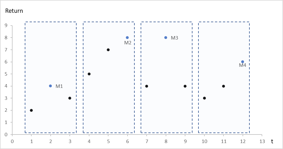
Source: computation by the author.

Figure 2. Illustration of the Peak-Over-Threshold approach

POT-GPD
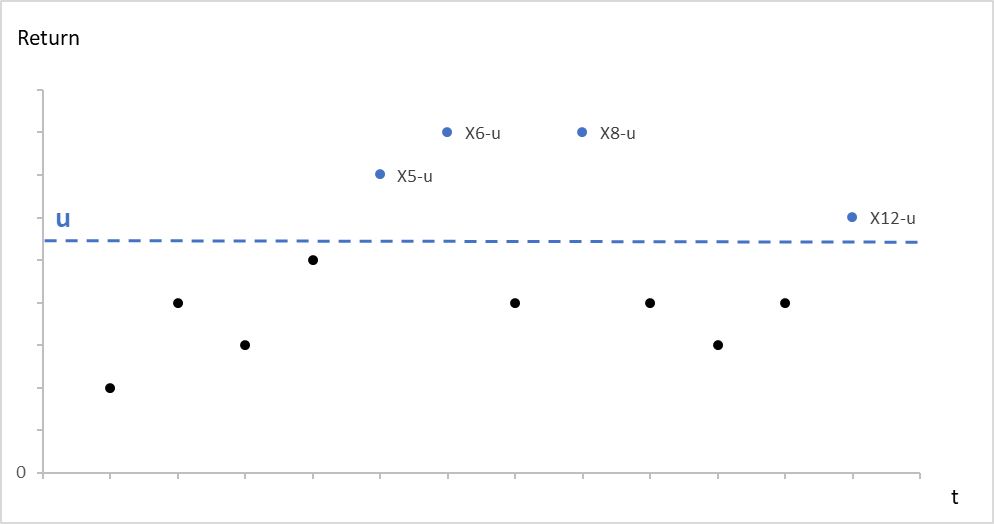
Source: computation by the author.

BM-GEV

Block-Maxima

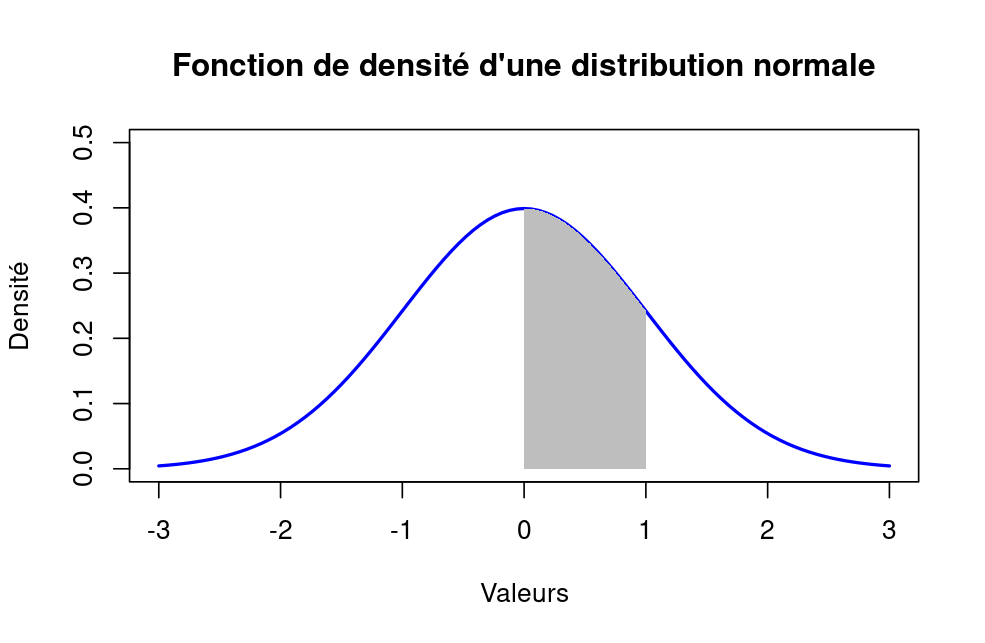
Let’s take a step back and have a look again at the Central Limit Theorem (CLT):

Illustration of the POT approach

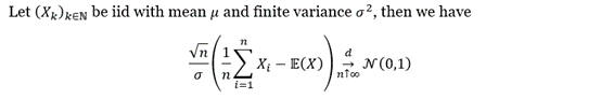
The CLT describes that the distribution of sample means approximates a normal distribution as the sample size gets larger. Similarly, the extreme value theory (EVT) studies the behavior of the extrema of samples.

The block maximum is defined as such:

Illustration of the POT approach

Generalized extreme value distribution (GEV)

Illustration of the POT approach

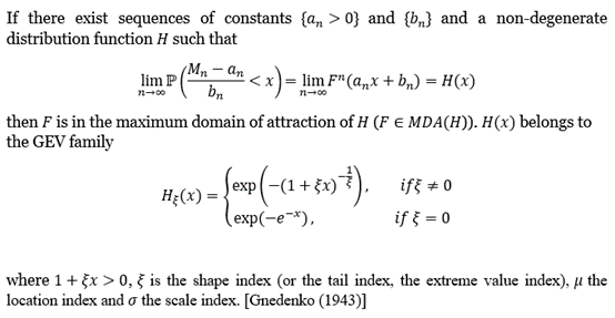
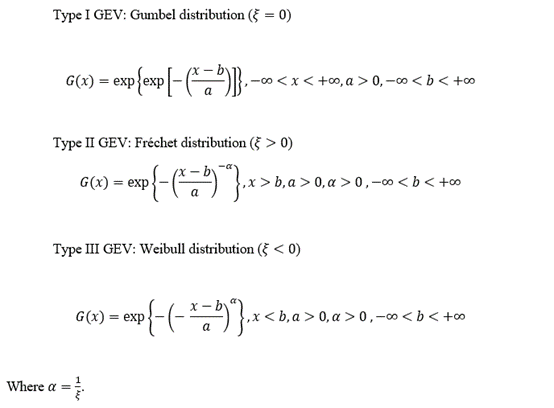
The GEV distributions have three subtypes corresponding to different tail feathers [von Misès (1936); Hosking et al. (1985)]:

Illustration of the POT approach

POT-GPD

The block maxima approach is under reproach for its inefficiency and wastefulness of data usage, and it has been largely superseded in practice by the peak-over-threshold (POT) approach. The POT approach makes use of all data entries above a designated high threshold u. The threshold exceedances could be fitted into a generalized Pareto distribution (GPD):

Illustration of the POT approach

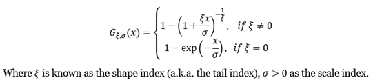
Illustration of Block Maxima and Peak-Over-Threshold approaches of the Extreme Value Theory with R

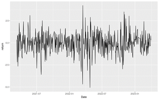
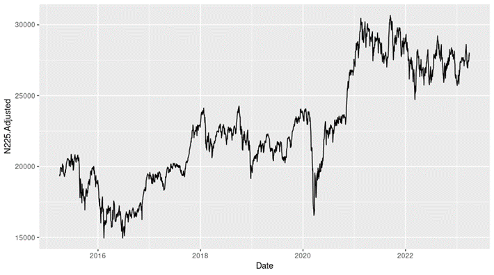
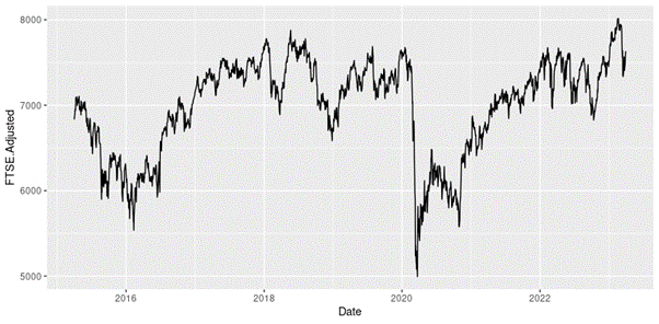
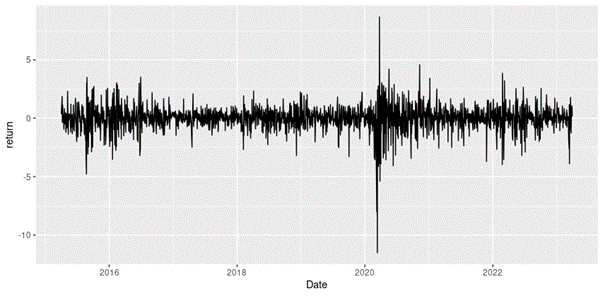
We now present an illustration of the two approaches of the extreme value theory (EVT), the block maxima with the generalized extreme value distribution (BM-GEV) approach and the peak-over-threshold with the generalized Pareto distribution (POT-GPD) approach, realized with R with the daily return data of the S&P 500 index from January 01, 1970, to August 31, 2022.

Packages and Libraries

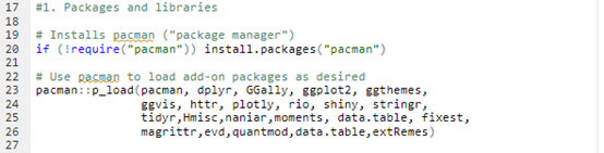
packages and libraries

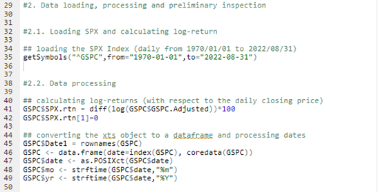
Data loading, processing and preliminary inspection

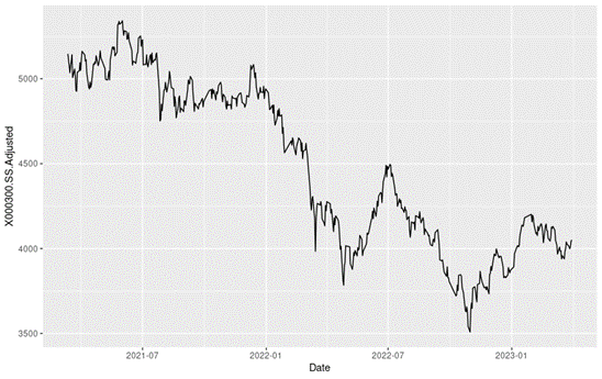
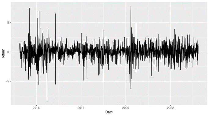
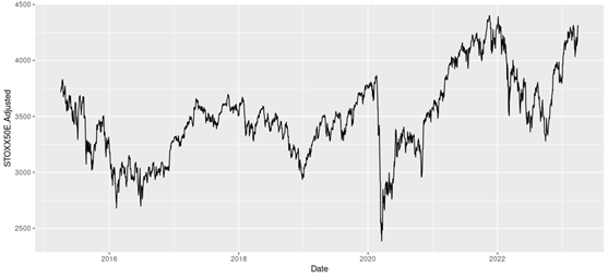
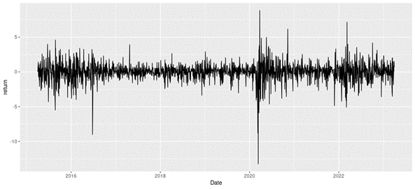
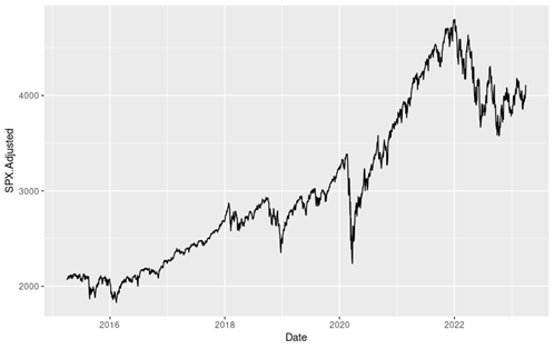
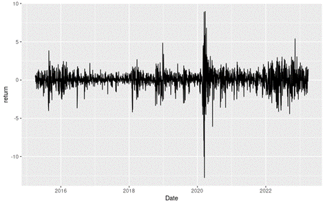
Loading S&P 500 daily closing prices from January 01, 1970, to August 31, 2022 and transforming the daily prices to daily logarithm returns (multiplied by 100). Month and year information are also extracted from later use.

data loading

Checking the preliminary statistics of the daily logarithm series.

descriptive stats data

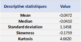
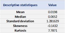
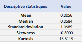
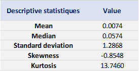
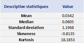
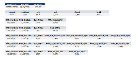
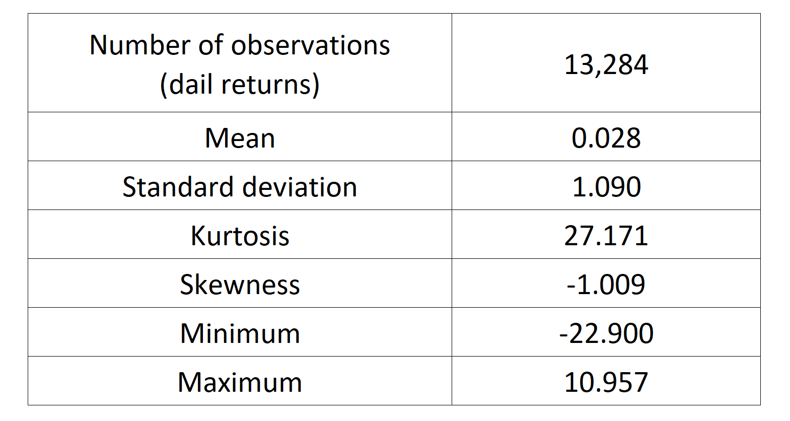
We can get the following basic statistics for the (logarithmic) daily returns of the S&P 500 index over the period from January 01, 1970, to August 31, 2022.

Table 1. Basic statistics of the daily return of the S&P 500 index.

Source: computation by the author.

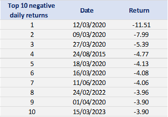
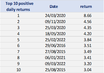
In terms of daily return, we can observe that the distribution is negatively skewed, which mean the negative tail is longer. The kurtosis is far higher than that of a normal distribution, which means that extreme outcomes are more frequent compared with a normal distribution. the minimum daily return is even more than twice of the maximum daily return, which could be interpreted as more prominent downside risk.

Block maxima – Generalized extreme value distribution (BM-GEV)

We define each month as a block and get the maxima from each block to study the behavior of the block maxima. We can also have a look at the descriptive statistics for the monthly downside extrema variable.

block maxima

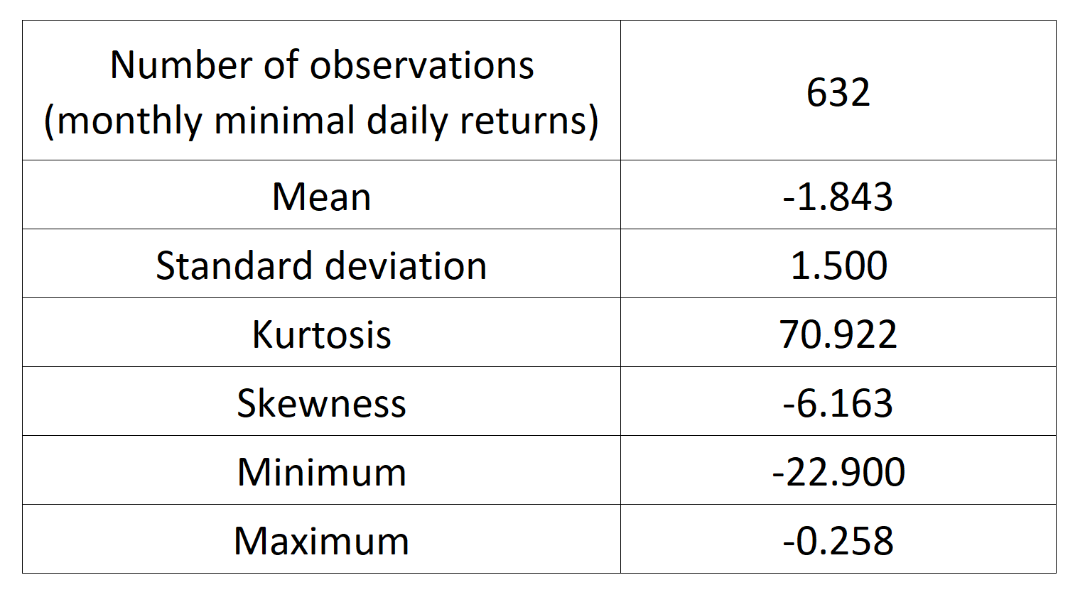
With the commands, we obtain the following basic statistics for the monthly minima variable:

Table 2. Basic statistics of the monthly minimal daily return of the S&P 500 index.

Source: computation by the author.

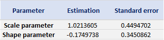
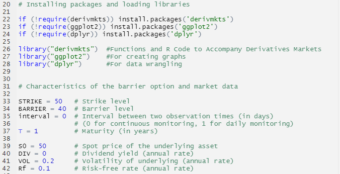
With the block extrema in hand, we can use the fevd() function from the extReme package to fit a GEV distribution. We can therefore get the following parameter estimations, with standard errors presented within brackets.

GEV

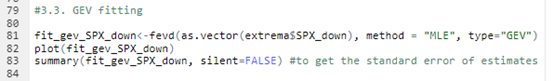
Table 3 gives the parameters estimation results of the generalized extreme value (GEV) for the monthly minimal daily returns of the S&P 500 index. The three parameters of the GEV distribution are the shape parameter, the location parameter and the scale parameter. For the period from January 01, 1970, to August 31, 2022, the estimation is based on 632 observations of monthly minimal daily returns.

Table 3. Parameters estimation results of GEV for the monthly minimal daily return of the S&P 500 index.

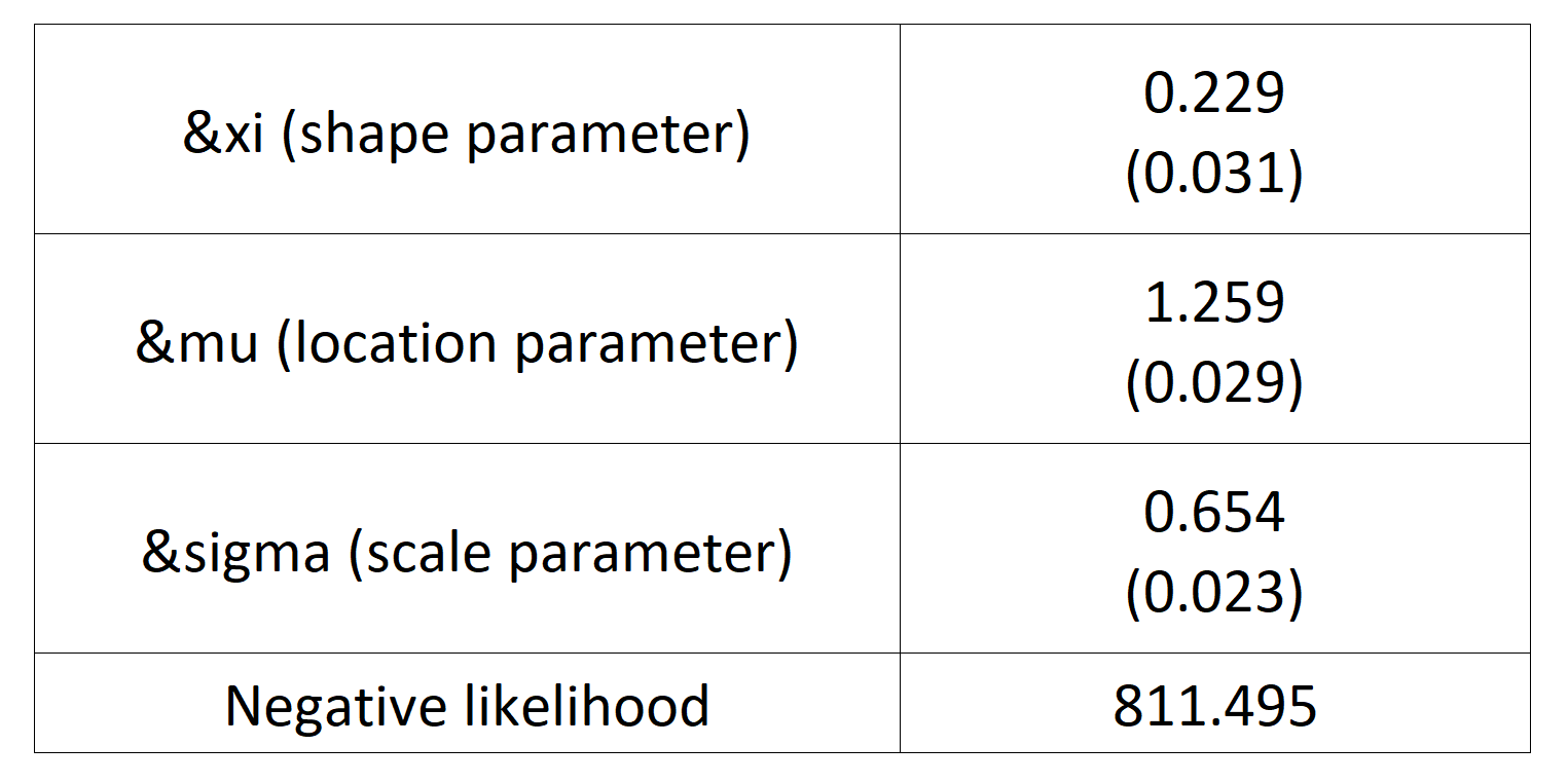
Source: computation by the author.

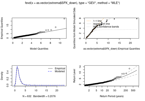
With the “plot” command, we are able to obtain the following diagrams.

The top two respectively compare empirical quantiles with model quantiles, and quantiles from model simulation with empirical quantiles. A good fit will yield a straight one-to-one line of points and in this case, the empirical quantiles fall in the 95% confidence bands.
The bottom left diagram is a density plot of empirical data and that of the fitted GEV distribution.
The bottom right diagram is a return period plot with 95% pointwise normal approximation confidence intervals. The return level plot consists of plotting the theoretical quantiles as a function of the return period with a logarithmic scale for the x-axis. For example, the 50-year return level is the level expected to be exceeded once every 50 years.

gev plots

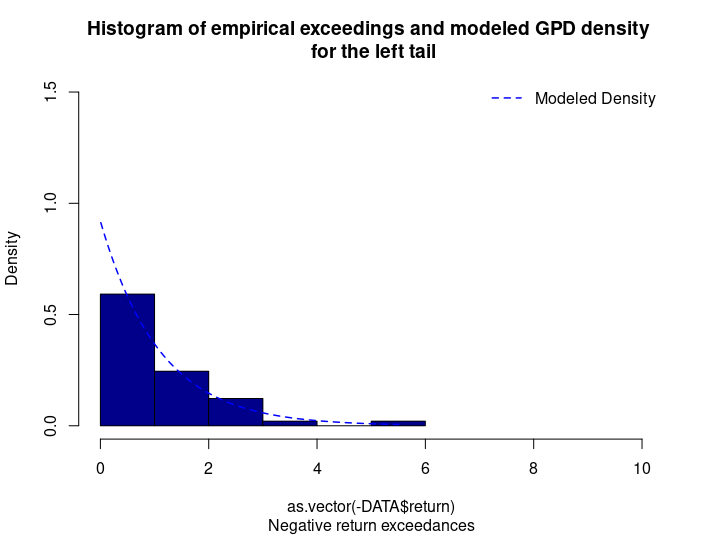
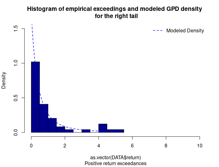
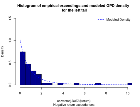
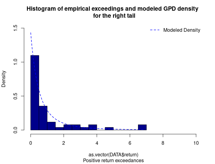
Peak over threshold – Generalized Pareto distribution (POT-GPD)

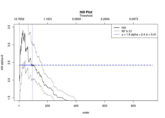
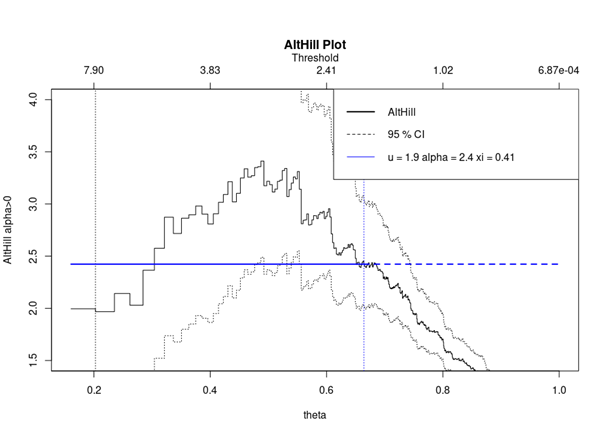
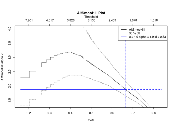
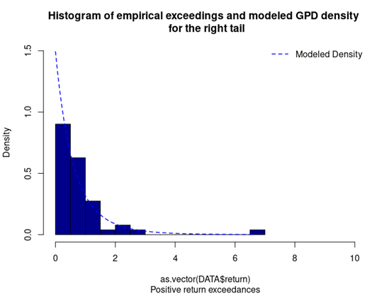
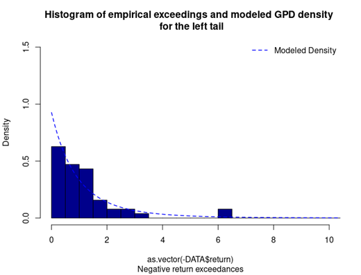
With respect to the POT approach, the threshold selection is central, and it involves a delicate trade-off between variance and bias where too high a threshold would reduce the number of exceedances and too low a threshold would incur a bias for poor GPD fitting (Rieder, 2014). The selection process could be elaborated in a separate post and here we use the optimal threshold of 0.010 (0.010*100 in this case since we multiply the logarithm return by 100) for stock index downside extreme movement proposed by Beirlant et al. (2004).

POT

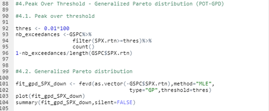
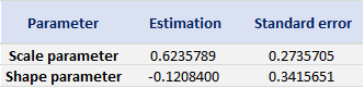
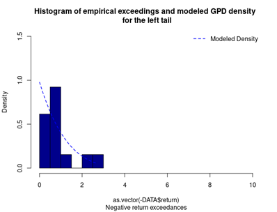
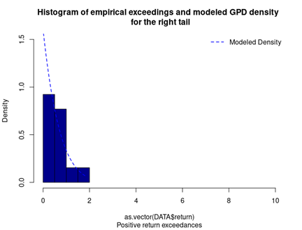
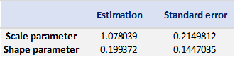
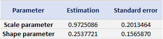
With the following commands, we get to fit the threshold exceedances to a generalized Pareto distribution, and we obtain the following parameter estimation results.

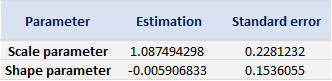
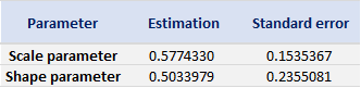
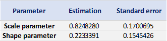
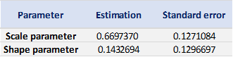
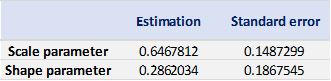
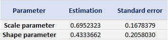
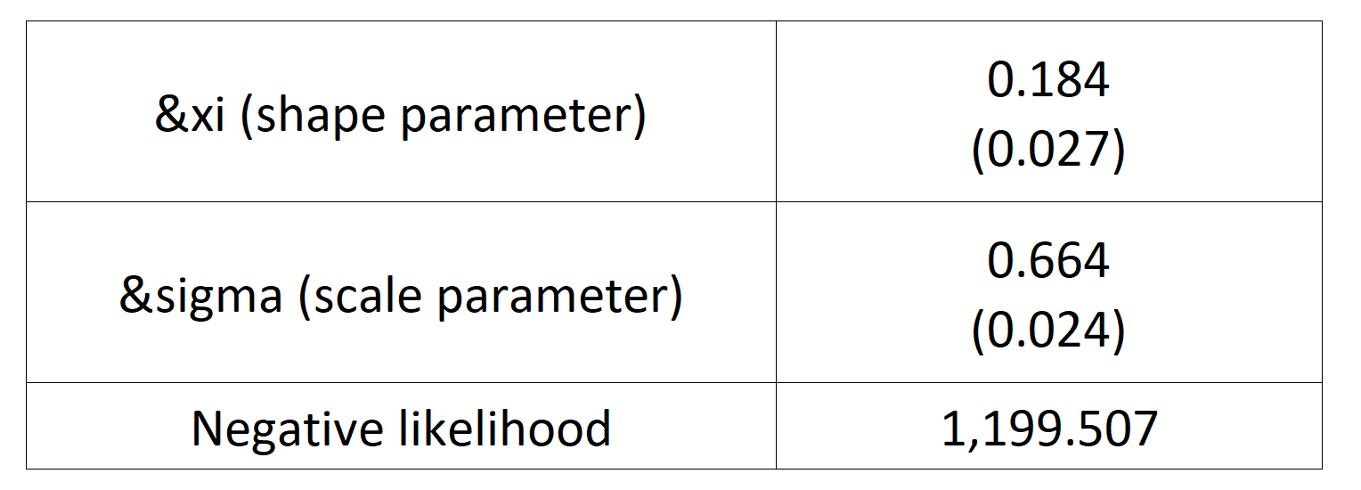
Table 4 gives the parameters estimation results of GPD for the daily return of the S&P 500 index with a threshold of -1%. In addition to the threshold, the two parameters of the GPD distribution are the shape parameter and the scale parameter. For the period from January 01, 1970, to August 31, 2022, the estimation is based on 1,669 observations of daily returns exceedances (12.66% of the total number of daily returns).

Table 4. Parameters estimation results of the generalized Pareto distribution (GPD) for the daily return negative exceedances of the S&P 500 index.

Source: computation by the author.

Download R file to understand the BM-GEV and POT-GPD approaches

You can find below an R file (file with txt format) to understand the BM-GEV and POT-GPD approaches.

Why should I be interested in this post

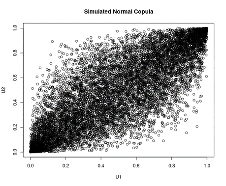
Financial crises arise alongside disruptive events such as pandemics, wars, or major market failures. The 2007-2008 financial crisis has been a recent and pertinent opportunity for market participants and academia to reflect on the causal factors to the crisis. The hindsight could be conducive to strengthening the market resilience faced with such events in the future and avoiding dire consequences that were previously witnessed. The Gaussian copula, a statistical tool used to manage the risk of the collateralized debt obligations (CDOs) that triggered the flare-up of the crisis, has been under serious reproach for its essential flaw to overlook the occurrence and the magnitude of extreme events. To effectively understand and cope with the extreme events, the extreme value theory (EVT), born in the 19th century, has regained its popularity and importance, especially amid the financial turmoil. Capital requirements for financial institutions, such as the Basel guidelines for banks and the Solvency II Directive for insurers, have their theoretical base in the EVT. It is therefore indispensable to be equipped with knowledge in the EVT for a better understanding of the multifold forms of risk that we are faced with.

Resources

Academic research (articles)

Aboura S. (2009) The extreme downside risk of the S&P 500 stock index. Journal of Financial Transformation, 2009, 26 (26), pp.104-107.

Gnedenko, B. (1943). Sur la distribution limite du terme maximum d’une série aléatoire. Annals of mathematics, 423–453.

Hosking, J. R. M., Wallis, J. R., & Wood, E. F. (1985) “Estimation of the generalized extreme-value distribution by the method of probability-weighted moments” Technometrics, 27(3), 251–261.

Longin F. (1996) The asymptotic distribution of extreme stock market returns Journal of Business, 63, 383-408.

Longin F. (2000) From VaR to stress testing : the extreme value approach Journal of Banking and Finance, 24, 1097-1130.

Longin F. et B. Solnik (2001) Extreme correlation of international equity markets Journal of Finance, 56, 651-678.

Mises, R. v. (1936). La distribution de la plus grande de n valeurs. Rev. math. Union interbalcanique, 1, 141–160.

Pickands III, J. (1975). Statistical Inference Using Extreme Order Statistics. The Annals of Statistics, 3(1), 119– 131.

Academic research (books)

Embrechts P., C. Klüppelberg and T Mikosch (1997) Modelling Extremal Events for Insurance and Finance.

Embrechts P., R. Frey, McNeil A. J. (2022) Quantitative Risk Management, Princeton University Press.

Gumbel, E. J. (1958) Statistics of extremes. New York: Columbia University Press.

Longin F. (2016) Extreme events in finance: a handbook of extreme value theory and its applications Wiley Editions.

Other materials

Extreme Events in Finance

Rieder H. E. (2014) Extreme Value Theory: A primer (slides).

About the author

The article was written in October 2022 by Shengyu ZHENG (ESSEC Business School, Grande Ecole Program – Master in Management, 2020-2023).

Reverse Convertibles

August 23, 2022 by Shengyu ZHENG

Reverse Convertibles

In this article, Shengyu ZHENG (ESSEC Business School, Grande Ecole Program – Master in Management, 2020-2023) explains reverse convertibles, which are a structured product with a fixed-rate coupon and downside risk.

Introduction

The financial market has been ever evolving, witnessing the birth and flourish of novel financial instruments to cater to the diverse needs of market participants. On top of plain vanilla derivative products, there are exotic ones (e.g., barrier options, the simplest and most traded exotic derivative product). Even more complex, there are structured products, which are essentially the combination of vanilla or exotic equity instruments and fixed income instruments.

Amongst the structured products, reverse convertible products are one of the most popular choices for investors. Reverse convertible products are non-principal protected products linked to the performance of an underlying asset, usually an individual stock or an index, or a basket of them. Clients can enter into a position of a reverse convertible with the over-the-counter (OTC) trading desks in major investment banks.

In exchange for an above-market coupon payment, the holder of the product gives up the potential upside exposure to the underlying asset. The exposure to the downside risks still remains. Reserve convertibles are therefore appreciated by the investors who are anticipating a stagnation or a slightly upward market trend.

Construction of a reverse convertible

This product could be decomposed in two parts:

On the one hand, the buyer of the structure receives coupons on the principal invested and this could be considered as a “coupon bond”;
On the other hand, the investor is still exposed to the downside risks of the underlying asset and foregoes the upside gains, and this could be achieved by a short position of a put option (either a vanilla put option or a down-and-in barrier put option).

Positions of the parties of the transaction

A reverse convertible involves two parties in the transaction: a market maker (investment bank) and an investor (client). Table 1 below describes the positions of the two parties at different time of the life cycle of the product.

Table 1. Positions of the parties of a reverse convertible transaction

t	Market Maker (Investment Bank)	Investor (Client)
Beginning	Enters into a long position of a put (either a vanilla put or a down-and-in barrier put) Receives the nominal amount for the “coupon” part Invests in the amount (nominal amount plus the premium of the put) in risk-free instruments	Enters into a short position of a put (either a vanilla put or a down-and-in barrier put) Pays the nominal amount for the “coupon” part
Interim	Pays pre-specified interim coupons in respective interim coupon payment dates (if any) Receives interest payment from risk-free investments	Receives the pre-specified interim coupons in respective interim coupon payment dates (if any)
End	Receives the payoff (if any) of the put option component Pays the pre-specified final coupon in the final coupon payment date	Pays the payoff (if any) of the put option component Receives the pre-specified final coupon in the final coupon payment date

Based on the type of the put option incorporated in the product (either plain vanilla put option or down-and-in barrier put option), reserve convertibles could be categorized as plain or barrier reverse convertibles. Given the difference in terms of the composition of the structured product, the payoff and pricing mechanisms diverge as well.

Here is an example of a plain reverse convertible with following product characteristics and market information.

Product characteristics:

Investment amount: USD 1,000,000.00
Underlying asset: S&P 500 index (Bloomberg Code: SPX Index)
Investment period: from August 12, 2022 to November 12, 2022 (3 months)
Coupon rate: 2.50% (quarterly)
Strike level : 100.00% of the initial level

Market data:

Current risk-free rate: 2.00% (annualized)
Volatility of the S&P 500 index: 13.00% (annualized)

Payoff of a plain reverse convertible

As is presented above, a reverse convertible is essentially a combination of a short position of a put option and a long position of a coupon bond. In case of the plain reverse convertible product with the aforementioned characteristics, we have the blow payoff structure:

in case of a rise of the S&P 500 index during the investment period, the return for the reverse convertible remains at 2.50% (the coupon rate);
in case of a drop of the S&P 500 index during the investment period, the return would be equal to 2.50% minus the percentage drop of the underlying asset and it could be negative if the percentage drop is greater than 2.5%.

Figure 1. The payoff of a plain reverse convertible on the S&P 500 index

Source: Computation by author.

Pricing of a plain reverse convertible

Since a reverse convertible is essentially a structured product composed of a put option and a coupon bond, the pricing of this product could also be decomposed into these two parts. In terms of the pricing a vanilla option, the Black–Scholes–Merton model could do the trick (see Black-Scholes-Merton option pricing model) and in terms of pricing a barrier option, two methods, analytical formula method and Monte-Carlo simulation method, could be of help (see Pricing barrier options with analytical formulas; Pricing barrier options with simulations and sensitivity analysis with Greeks).

With the given parameters, we can calculate, as follows, the margin for the bank with respect to this product. The calculated margin could be considered as the theoretical price of this product.

Table 2. Margin for the bank for the plain reverse convertible

Source: Computation by author.

Download the Excel file to analyze reverse convertibles

You can find below an Excel file to analyze reverse convertibles.

Why should I be interested in this post

As one of the most traded structured products, reverse convertibles have been an important instrument used to secure return amid mildly negative market prospect. It is, therefore, helpful to understand the product elements, such as the construction and the payoff of the product and the targeted clients. This could act as a steppingstone to financial product engineering and risk management.

Resources

Academic references

Broadie, M., Glasserman P., Kou S. (1997) A Continuity Correction for Discrete Barrier Option. Mathematical Finance, 7:325-349.

De Bellefroid, M. (2017) Chapter 13 (Barrier) Reverse Convertibles. The Derivatives Academy. Accessible at https://bookdown.org/maxime_debellefroid/MyBook/barrier-reverse-convertibles.html

Haug, E. (1997) The Complete Guide to Option Pricing. London/New York: McGraw-Hill.

Hull, J. (2006) Options, Futures, and Other Derivatives. Upper Saddle River, N.J: Pearson/Prentice Hall.

Merton, R. (1973). Theory of Rational Option Pricing. The Bell Journal of Economics and Management Science, 4:141-183.

Paixao, T. (2012) A Guide to Structured Products – Reverse Convertible on S&P500

Reiner, E. S. (1991) Breaking down the barriers. Risk Magazine, 4(8), 28–35.

Rich, D.R. (1994) The Mathematical Foundations of Barrier Option-Pricing Theory. Advances in Futures and Options Research: A Research Annual, 7, 267-311.

Business references

Six Structured Products. (2022). Reverse Convertibles et barrier reverse Convertibles

About the author

The article was written in August 2022 by Shengyu ZHENG (ESSEC Business School, Grande Ecole Program – Master in Management, 2020-2023).

Pricing barrier options with simulations and sensitivity analysis with Greeks

July 10, 2022 by Shengyu ZHENG

Pricing barrier options with simulations and sensitivity analysis with Greeks

In this article, Shengyu ZHENG (ESSEC Business School, Grande Ecole Program – Master in Management, 2020-2023) explains the pricing of barrier options with Monte-Carlo simulations and the sensitivity analysis of barrier options from the perspective of Greeks.

Pricing of discretely monitored barrier options with Monte-Carlo simulations

With the simulation method, only the pricing of discretely monitored barrier options can be handled since it is impossible to simulate continuous price trajectories with no intervals. Here the method is illustrated with a down-and-out put option. The general setup of economic details of the down-and-out put option and related market information are presented as follows:

General setup of simulation for barrier option pricing

Similar to the simulation method for pricing standard vanilla options, Monte Carlo simulations based on Geometric Brownian Motion could also be employed to analyze the pricing of barrier options.

Figure 1. Trajectories of 600 price simulations.

With the R script presented above, we can simulate 6,000 times with the simprice() function from the derivmkts package. Trajectories of 600 price simulations are presented above, with the black line representing the mean of the final prices, the green dashed lines 1x and 2x standard deviation above the mean, the red dashed lines 1x and 2x derivation below the mean, the blue dashed line the strike level and the brown line the knock-out level.

The simprice() function, according to the documentation, computes simulated lognormal price paths with the given parameters.

With this simulation of 6,000 price paths, we arrive at a price of 0.6720201, which is quite close to the one calculated from the formulaic approach from the previous post.

Analysis of Greeks

The Greeks are the measures representing the sensitivity of the price of derivative products including options to a change in parameters such as the price and the volatility of the underlying asset, the risk-free interest rate, the passage of time, etc. Greeks are important elements to look at for risk management and hedging purposes, especially for market makers (dealers) since they do not essentially take these risks for themselves.

In R, with the combination of the greeks() function and a barrier pricing function, putdownout() in this case, we can easily arrive at the Greeks for this option.

Barrier option R code Sensitivity Greeks

Table 1. Greeks of the Down-and-Out Put

Barrier Option Greeks Summary

We can also have a look at the evolutions of the Greeks with the change of one of the parameters. The following R script presents an example of the evolutions of the Greeks along with the changes in the strike price of the down-and-out put option.

Barrier option R code Sensitivity Greeks Evolution

Figure 2. Evolution of Greeks with the change of Strike Price of a Down-and-Out Put

Evolution Greeks Barrier Price

Download R file to price barrier options

You can find below an R file (file with txt format) to price barrier options.

Why should I be interested in this post?

As one of the most traded but the simplest exotic derivative products, barrier options open an avenue for different applications. They are also very often incorporated in structured products, such as reverse convertibles. It is, therefore, important to be equipped with knowledge of this product and to understand the pricing logics if one aspires to work in the domain of market finance.

Simulation methods are very common in pricing derivative products, especially for those without closed-formed pricing formulas. This post only presents a simple example of pricing barrier options and much optimization is needed for pricing more complex products with more rounds of simulations.

Useful resources

Academic articles

Broadie, M., Glasserman P., Kou S. (1997) A Continuity Correction for Discrete Barrier Option. Mathematical Finance, 7:325-349.

Merton, R. (1973) Theory of Rational Option Pricing. The Bell Journal of Economics and Management Science, 4:141-183.

Paixao, T. (2012) A Guide to Structured Products – Reverse Convertible on S&P500

Reiner, E.S., Rubinstein, M. (1991) Breaking down the barriers. Risk Magazine, 4(8), 28–35.

Rich, D. R. (1994) The Mathematical Foundations of Barrier Option-Pricing Theory. Advances in Futures and Options Research: A Research Annual, 7:267-311.

Wang, B., Wang, L. (2011) Pricing Barrier Options using Monte Carlo Methods, Working paper.

Books

Haug, E. (1997) The Complete Guide to Option Pricing. London/New York: McGraw-Hill.

Hull, J. (2006) Options, Futures, and Other Derivatives. Upper Saddle River, N.J: Pearson/Prentice Hall.

About the author

The article was written in June 2022 by Shengyu ZHENG (ESSEC Business School, Grande Ecole Program – Master in Management, 2020-2023).

Pricing barrier options with analytical formulas

February 5, 2024July 10, 2022 by Shengyu ZHENG

Pricing barrier options with analytical formulas

As is mentioned in the previous post, the frequency of monitoring is one of the determinants of the price of a barrier option. The higher the frequency, the more likely a barrier event would take place.

In this article, Shengyu ZHENG (ESSEC Business School, Grande Ecole Program – Master in Management, 2020-2023) explains the pricing of continuously and discretely monitored barrier options with analytical formulas.

Pricing of standard continuously monitored barrier options

For pricing standard barrier options, we cannot simply apply the Black-Sholes-Merton Formula for the particularity of the barrier conditions. There are, however, several models available developed on top of this theoretical basis. Among them, models developed by Merton (1973), Reiner and Rubinstein (1991) and Rich (1994) enabled the pricing of continuously monitored barrier options to be conducted in a formulaic fashion. They are concisely put together by Haug (1997) as follows:

Knock-in and knock-out barrier option pricing formula

Knock-in barrier option pricing formula

Pricing of standard discretely monitored barrier options

For discretely monitored barrier options, Broadie and Glasserman (1997) derived an adjustment that is applicable on top of the pricing formulas of the continuously monitored counterparts.

Let’s denote:

Knock-in barrier option pricing formula

The price of a discretely monitored barrier option of a certain barrier price equals the price of a continuously monitored barrier option of the adjusted price plus an error:

Knock-in barrier option pricing formula

The adjusted barrier price, in this case, would be:

Knock-in barrier option pricing formula

It is also worth noting that the error term o(·) grows prominently when the barrier approaches the strike price. A threshold of 5% from the strike price should be imposed if this approach is employed for pricing discretely monitored barrier options.

Example of pricing a down-and-out put with R with the formulaic approach

The general setup of economic details of the Down-and-Out Put and related market information is presented as follows:

Knock-in barrier option pricing formula

There are built-in functions in the “derivmkts” library that render directly the prices of barrier options of continuous monitoring, such as calldownin(), callupin(), calldownout(), callupout(), putdownin(), putupin(), putdownout(), and putupout (). By incorporating the adjustment proposed by Broadie and Glasserman (1997), all barrier options of both monitoring methods could be priced in a formulaic way with the following function:

Knock-in barrier option pricing formula

For example, for a down-and-out Put option with the aforementioned parameters, we can use this function to calculate the prices.

Knock-in barrier option pricing formula

For continuous monitoring, we get a price of 0.6264298, and for daily discrete monitoring, we get a price of 0.676141. It makes sense that for a down-and-out put option, a lower frequency of barrier monitoring means less probability of a knock-out event, thus less protection for the seller from extreme downside price trajectories. Therefore, the seller would charge a higher premium for this put option.

Download R file to price barrier options

You can find below an R file (file with txt format) to price barrier options.

Why should I be interested in this post?

As one of the most traded but the simplest exotic derivative products, barrier options open an avenue for different applications. They are also very often incorporated in structured products, such as reverse convertibles. It is, therefore, important to understand the elements having an impact on their prices and the closed-form pricing formulas are a good presentation of these elements.

Useful resources

Academic research articles

Broadie, M., Glasserman P., Kou S. (1997) A Continuity Correction for Discrete Barrier Option. Mathematical Finance, 7:325-349.

Merton, R. (1973) Theory of Rational Option Pricing. The Bell Journal of Economics and Management Science, 4:141-183.

Paixao, T. (2012) A Guide to Structured Products – Reverse Convertible on S&P500

Reiner, E.S., Rubinstein, M. (1991) Breaking down the barriers. Risk Magazine, 4(8), 28–35.

Rich, D. R. (1994) The Mathematical Foundations of Barrier Option-Pricing Theory. Advances in Futures and Options Research: A Research Annual, 7:267-311.

Wang, B., Wang, L. (2011) Pricing Barrier Options using Monte Carlo Methods, Working paper.

Books

Haug, E. (1997) The Complete Guide to Option Pricing. London/New York: McGraw-Hill.

Hull, J. (2006) Options, Futures, and Other Derivatives. Upper Saddle River, N.J: Pearson/Prentice Hall.

About the author

The article was written in July 2022 by Shengyu ZHENG (ESSEC Business School, Grande Ecole Program – Master in Management, 2020-2023).

Barrier options

July 6, 2022 by Shengyu ZHENG

Barrier options

In this article, Shengyu ZHENG (ESSEC Business School, Grande Ecole Program – Master in Management, 2020-2023) explains barrier options which are the most traded exotic options in derivatives markets.

Description

Barrier options are path dependent. Their payoffs are not only a function of the price of the underlying asset relative to the option strike, but also depend on whether the price of the underlying asset reached a certain predefined barrier during the life of the option.

The two most common kinds of barrier options are knock-in (KI) and knock-out (KO) options.

Knock-in (KI) barrier options

KI barrier options are options that are activated only if the underlying asset attains a prespecified barrier level (the “knock-in” event). With the absence of this knock-in event, the payoff remains zero regardless of the trajectory of the price of the underlying asset.

Knock-out (KO) barrier options

KO barrier options are options that are deactivated only if the underlying asset attains a prespecified barrier level (the “knock-out” event). In the presence of this knock-out event, the payoff remains zero regardless of the trajectory of the price of the underlying asset.

Observation

The determination of the occurrence of a barrier event (KI or KO conditions) is essential to the ultimate payoff of the barrier option. In practice, the details of the KI or KO conditions are precisely defined in the contract (called “Confirmations” by the International Swaps and Derivatives Association (ISDA) for over-the counter (OTC) traded options).

Observation period

The observation period denotes the period where a barrier event (KI or KO) can be observed, that is to say, when the price of the underlying asset is monitored. There are three styles of observation period: European style, partial-period American style, and full-period American style.

European style: The observation period is only the expiration date of the barrier option.
Partial-period American style: The observation period is part of the lifespan of the barrier option.
Full-period American style: The observation period spans the whole period from the effective date to the expiration date of the barrier option.

Monitoring method

There are two typical types of monitoring methods in terms of the determination of a knock-in/knock-out event: continuous monitoring and discrete monitoring. The monitoring method is one of the key factors in determining the premium of a barrier option.

Continuous monitoring: A knock-in/knock-out event is deemed to take place if, at any time in the observation period, the knock-in/knock-out condition is met.
Discrete monitoring: A knock-in/knock-out event is deemed to occur if, at pre-specific times in the observation period, usually the closing time of each trading day, the knock-in/knock-out condition is met.

Barrier Reference Asset

For the most cases, the Barrier Reference Asset is the underlying asset itself. However, if specified in the contract, it can be another asset or index. It can also be other calculatable properties, such as the volatility of the asset. In this case, the methodology of calculating such properties should be clearly defined in the contract.

Rebate

For knock-out options, there could be a rebate. A rebate is an extra feature and it corresponds to the amount that should be paid to the buyer of the knock-out option in case of the occurrence of a knock-out event.

In-out parity relation for barrier options

Analogous to the call-put parity relation for plain vanilla options, there is an in-out parity relation for barrier options stating that a long position in a knock-in option plus a long position in a knock-out option with identical strikes, barriers, monitoring methods and maturity is equivalent to a long position in a comparable vanilla option. It could be stated as follows:

Knock-in knock-out barrier option parity relation

Where K denotes the strike price, T the maturity, and B the barrier level.

It is worth noting that this parity relation is valid only when the two KI and KO options are identical, and there is no rebate in case of a knock-out option.

Basic barrier options

There are four types of basic barrier options traded in the market: up-and-in option, up-and-out option, down-and-in option, and down-and-out option. “Up” and “down” denotes the direction of surpassing the barrier price. “In” and “out” depict the type of barrier condition, i.e. knock-in or knock-out. These four types of barrier features are available for both call and put options.

Up-and-in option

An up-and-in option is a knock-in option whose barrier condition is achieved if the underlying price arrives higher than the barrier level during the observation period.

Figure 1 illustrates the occurrence of an up-and-in barrier event for a barrier option with full-period American style and discrete monitoring (the closing time of each trading day).

Figure 1. Illustration of an up-and-in barrier option
Example of an up-and-in call option

Up-and-out option

An up-and-out option is a knock-out option whose barrier condition is achieved if the underlying price arrives higher than the barrier level during the observation period.

Figure 2. Illustration of an up-and-out option

Example of an up-and-out call option

Down-and-in option

A down-and-in option is a knock-in option whose barrier condition is achieved if the underlying price arrives lower than the barrier level during the observation period.

Figure 3. Illustration of a down-and-in option
Example of a down-and-in call option

Down-and-out option

A down-and-out option is a knock-out option whose barrier condition is achieved if the underlying price arrives lower than the barrier level during the observation period.

Figure 4. Illustration of a down-and-out option
Example of a down-and-out call option

Download R file to price barrier options

You can find below an R file to price barrier options.

Trading of barrier options

Being the most popular exotic options, barrier options on stocks or indices have been actively traded in the OTC market since the inception of the market. Unavailable in standard exchanges, they are less accessible than their vanilla counterparts. Barrier options are also commonly utilized in structured products.

Why should I be interested in this post?

As one of the most traded but the simplest exotic derivative products, barrier options open an avenue for different applications. They are also very often incorporated in structured products, such as reverse convertibles. Knock-in/knock out conditions are also common features in other types of more complicated exotic derivative products.

It is, therefore, important to be equipped with knowledge of this product and to understand the pricing logics if one aspires to work in financial markets.

References

Academic research articles

Broadie, M., Glasserman P., Kou S. (1997) A Continuity Correction for Discrete Barrier Option. Mathematical Finance, 7:325-349.

Merton, R. (1973) Theory of Rational Option Pricing. The Bell Journal of Economics and Management Science, 4:141-183.

Paixao, T. (2012) A Guide to Structured Products – Reverse Convertible on S&P500

Reiner, E.S., Rubinstein, M. (1991) Breaking down the barriers. Risk Magazine, 4(8), 28–35.

Rich, D. R. (1994) The Mathematical Foundations of Barrier Option-Pricing Theory. Advances in Futures and Options Research: A Research Annual, 7:267-311.

Wang, B., Wang, L. (2011) Pricing Barrier Options using Monte Carlo Methods, Working paper.

Books

Haug, E. (1997) The Complete Guide to Option Pricing. London/New York: McGraw-Hill.

Hull, J. (2006) Options, Futures, and Other Derivatives. Upper Saddle River, N.J: Pearson/Prentice Hall.

About the author

The article was written in July 2022 by Shengyu ZHENG (ESSEC Business School, Grande Ecole Program – Master in Management, 2020-2023).

Extreme correlation

Background

Linear correlation and copula

Tail dependence coefficient

Examples of extreme correlation

Related posts on the SimTrade blog

About extreme value theory

Useful resources

Academic resources

Other resources

About the author

Optimal threshold selection for the peak-over-threshold approach of extreme value theory

The Peak-over-Threshold threshold approach

Threshold selection

Methods of optimal threshold selection

Plot analysis

Monte Carlo simulations

Other methods

Download R file to model extreme behavior of the index

Related posts about extreme value theory

Useful resources

Academic resources

Other resources

About the author

Extreme returns and tail modelling of the CSI 300 index for the Chinese equity market

The CSI 300 index for the Chinese equity market

Summary statistics for the CSI 300 index

Modelling of the tails

Applications in risk management

Why should I be interested in this post?

Download R file to model extreme behavior of the index

Related posts on the SimTrade blog

About financial indexes

About portfolio management

About statistics

Useful resources

Academic resources

Other resources

About the author

Extreme returns and tail modelling of the Nikkei 225 index for the Japanese equity market

The Nikkei 225 index for the Japanese equity market

Summary statistics for the Nikkei index

Modelling of the tails

Applications in risk management

Why should I be interested in this post?

Download R file to model extreme behavior of the index

Related posts on the SimTrade blog

About financial indexes

About portfolio management

About statistics

Useful resources

Academic resources

Other resources

About the author

Extreme returns and tail modelling of the FTSE 100 index for the UK equity market

The FTSE 100 index for the UK equity market

Summary statistics for the FTSE 100 index

Modelling of the tails

Applications in risk management

Why should I be interested in this post?

Download R file to model extreme behavior of the index

Related posts on the SimTrade blog

About financial indexes

About portfolio management

About statistics

Useful resources

Academic resources

Other resources

About the author

Copula

Linear correlation

Definition of linear correlation

Limitation of linear correlation

Copula

Definition of copula

Fréchet-Hoeffding bounds

Sklar’s theorem

Examples of copulas

Elliptical or normal copulas

Archimedean copulas