Interest Rate Swaps

December 29, 2022 by Akshit GUPTA

This article written by Akshit GUPTA (ESSEC Business School, Grande Ecole Program – Master in Management, 2019-2022) presents the derivative contract of interest rate swaps used to hedge interest rate risk in financial markets.

Introduction

In financial markets, interest rate swaps are derivative contracts used by two counterparties to exchange a stream of future interest payments with another for a pre-defined number of years. The interest payments are based on a pre-determined notional principal amount and usually include the exchange of a fixed interest rate for a floating interest rate (or sometimes the exchange of a floating interest rate for another floating interest rate).

While hedging does not necessarily eliminate the entire risk for any investment, it does limit or offset any potential losses that the investor can incur.

Forward rate agreements (FRA)

To understand interest rate swaps, we first need to understand forward rate agreements in financial markets.

In an FRA, two counterparties agree to an exchange of cashflows in the future based on two different interest rates, one of which is a fixed rate and the other is a floating rate. The interest rate payments are based on a pre-determined notional amount and maturity period. This derivative contract has a single settlement date. LIBOR (London Interbank Offered Rate) is frequently used as the floating rate index to determine the floating interest rate in the swap.

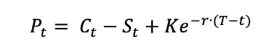
The payoff of the contract is as shown in the formula below:

(LIBOR – Fixed Interest Rate) * Notional amount * Number of days / 100

Interest rate swaps (IRS)

An interest rate swap is a hedging mechanism wherein a pre-defined series of forward rate agreements to buy or sell the floating interest rate at the same fixed interest rate.

In an interest rate swap, the position taken by the receiver of the fixed interest rate is called “long receiver swaps” and the position taken by the payer of the fixed interest rate is called “long payer swaps”.

How does an interest rate swap work?

Interest rate swaps can be used in different market situations based on a counterparty’s prediction about future interest rates.

For example, when a firm paying a fixed rate of interest on an existing loan believes that the interest rate will decrease in the future, it may enter an interest rate swap agreement in which it pays a floating rate and receives a fixed rate to benefit from its expectation about the path of future interest rates. Conversely, if the firm paying a floating interest rate on an existing loan believes that the interest rate will increase in the future, it may enter an interest rate swap in which it pays a fixed rate and receives a floating rate to benefit from its expectation about the path of future interest rates.

Example

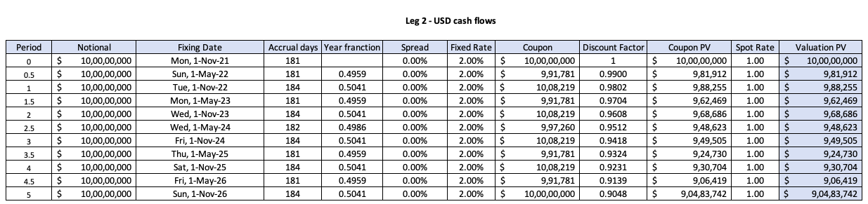
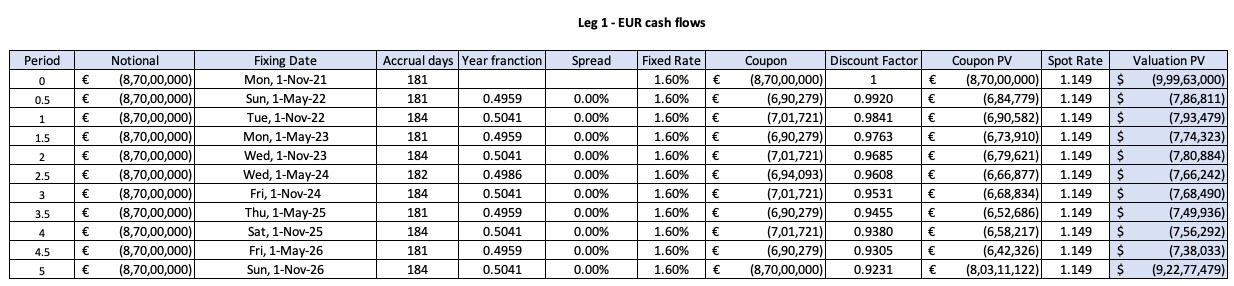
Let’s consider a 4-year swap between two counterparties A and B on January 1, 2021. In this swap, counterparty A agrees to pay a fixed interest rate of 3.60% per annum to counterparty B every six months on an agreed notional amount of €10 million. Counterparty B agrees to pay a floating interest rate based on the 6-month LIBOR rate, currently at 2.60%, to Counterparty A on the same notional amount. Here, the position taken by Counterparty A is called long payer swap and the position taken by Counterparty B is called the long receiver swap. The projected cashflow receipt to Counterparty A based on the assumed LIBOR rates is shown in the below table:

Table 1. Cash flows for an interest rate swap.

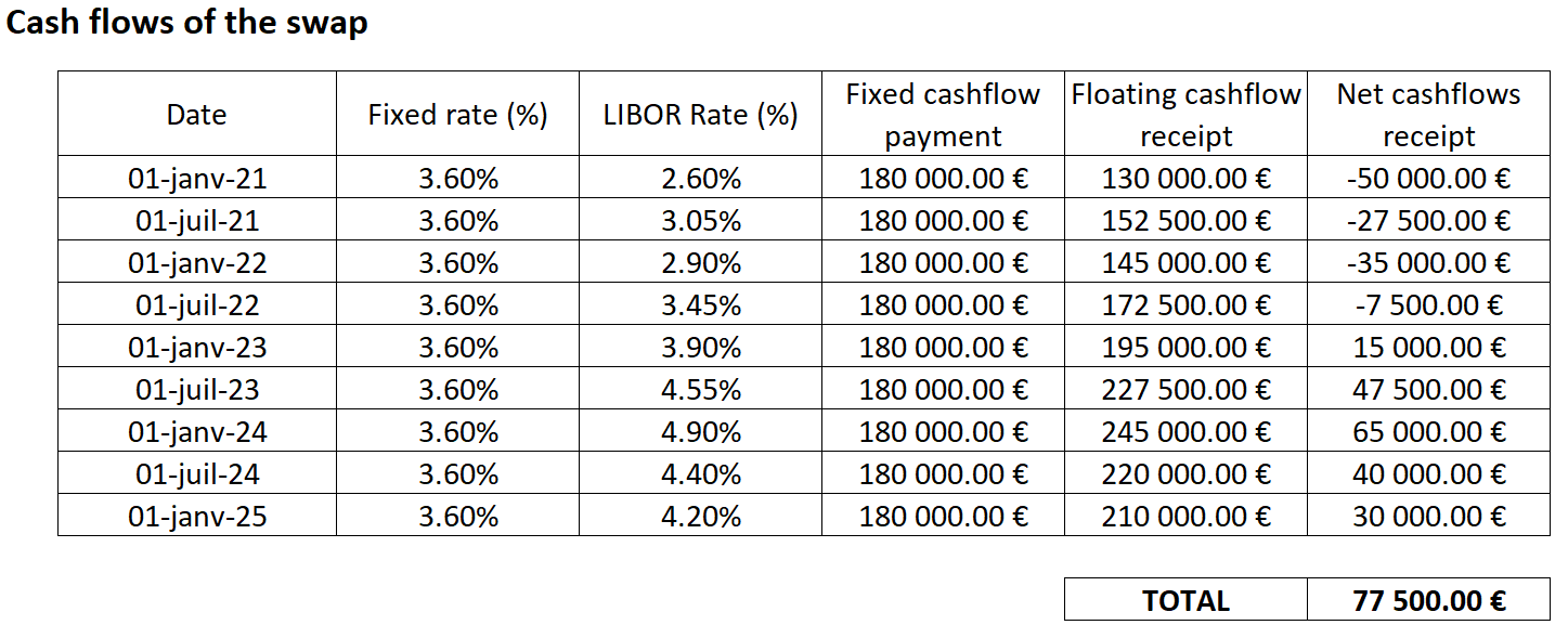
Source: computation by the author

In the above example, a total of eight payments (two per year) are made on the interest rate swap. The fixed rate payment is fixed at €180,000 per observation date whereas the floating payment rate depend on the prevailing LIBOR rate at the observation date. The net receipt for the Counterparty A is equal to €77,500 at the end of 5 years. Note that in an interest rate swap the notional amount of €10 million is not exchanged between the counterparties since it has no financial value to either of the counterparties and that is why it is called the “notional amount”.

Note that when the two counterparties enter the swap, the fixed rate is set such that the swap value is equal to zero.

Excel file for interest rate swaps

You can download below the Excel file for the computation of the cash flows for an interest rate swap.

▶ Jayati WALIA Derivative Markets

▶ Akshit GUPTA Forward Contracts

▶ Akshit GUPTA Options

Useful resources

Hull J.C. (2015) Options, Futures, and Other Derivatives, Ninth Edition, Chapter 7 – Swaps, 180-211.

www.longin.fr Pricer of interest swaps

About the author

Article written in December 2022 by Akshit GUPTA (ESSEC Business School, Grande Ecole Program – Master in Management, 2019-2022).

My apprenticeship experience within client services at BNP Paribas

December 29, 2022 by Akshit GUPTA

In this article Akshit GUPTA (ESSEC Business School, Grande Ecole Program – Master in Management, 2019-2022) shares his apprenticeship experience as a client services analyst at BNP Paribas, which is the leading European banking group.

Introduction

BNP Paribas is a French banking group which was formed as a result of a merger between Banque Nationale de Paris (BNP) and Paribas in the year 2000. The group’s business is divided in 3 major operating divisions including: Commercial, Personal Banking & Services (CPBS), Investment & Protection Services (IPS) and Corporate Institutional Banking (CIB) and the bank has its presence in 65 countries.

BNP Paribas Logo

BNP Paribas is ranked as the largest banking group in Europe and amongst top 10 in the world in terms of total assets which reflects the size of financial institution. BNP Paribas is a publicly listed company on Euronext Paris and is a part of the CAC 40 and Euro Stoxx 50 index.

Table 1. Ranking of banks by total assets

BNP Paribas Ranking

Source: www.advratings.com

My Apprenticeship Experience

I worked as a Client Services Analyst within the Corporate and Institutional Banking (CIB) division of the bank.

Missions

I had the opportunity to undertake two missions during the apprenticeship at BNP Paribas. During my first year, I worked as a Client Services Officer in the Factsheets team wherein I was responsible for creating and producing factsheets on equity and fixed income linked structured products and custom indices for the institutional clients of the bank. The Client Services is a cross functional team within the BNP Paribas Global Markets. They aim to provide the clients with the best possible post-trade service on the global market activity of the bank. The team works in close coordination with various teams operating on the capital markets (Sales, Traders, Business Managers, Middle and Back Office, Compliance, and Lawyers) and on all types of products (equities, fixed income, commodities, foreign exchange, and derivatives).

My work involved analysing the technical term-sheets (documents which present technical information about the products) of different structured products and produce factsheets (documents which mainly present the financial performance of the products) related to these products in conjunction with the Structuring and Sales teams at the bank. The factsheets were automated and produced on different frequencies like daily, weekly, bi-weekly, and monthly to serve the needs of different clients. These reports included products’ performance measures, and commentary on market data and current economic scenarios on these products.

During the second year of my apprenticeship, I worked as an Operational Client Relationship Manager (OCRM) within the same division at BNP Paribas but with a change of business responsibilities and duties to gain more exposure on the client facing side of the business.

In this role, I was responsible for developing and maintaining strong commercial relationships with the top institutional clients of our bank and manage client’s transversal escalations for multi asset classes including Equities, Fixed Income, Foreign Exchange, and Credit Derivatives. I worked on pre and post trade issues in close coordination with cross functional teams like Sales, Trading, Onboarding, Legal, Compliance and Operations to resolve breaks and efficiently serve the clients.

Required skills and knowledge

Strong knowledge of investment banking, equity, and capital markets.
Strong skillset in MS Office pack including MS Excel, MS Word, MS Access, and MS PowerPoint to produce reports and KPI dashboards for internal and external purposes.
Familiarity with programming in VBA and SQL.
Understanding of front-to-back trade lifecycle of different products.
Effective communication skills to interact with clients and internal stakeholders
Strong interpersonal skills.

What I learnt?

With this apprenticeship experience, I gained strong exposure to the different structured products issued by a bank like BNP Paribas in the global markets, understanding of client communication side, and programming skills in VBA and SQL. Along with the technical skillsets, I also learnt the importance of working as a team, understanding each other’s viewpoints, and aiming towards a common goal. It brought into focus the importance of banking sector and has given me a platform to sharpen my financial acumen.

Key concepts

The following are the two concepts that were required in my work at BNP Paribas:

Global markets

Global Markets is a division within an investment bank which handles all the sales and trading services on both the primary and secondary markets for different financial products. It caters to different clients including financial institutions, corporates and large-scale investors. The teams within this division are generally split based on different asset classes. Relevant knowledge of the different functions within this division is important to facilitate and coordinate client escalations and projects.

Structured products

Structured products are pre-packaged product offerings which are designed as per the client’s risk-return profile. The returns on the investments in these products are based on the performance of the underlying assets. These underlying assets can include individual assets or indices in various markets like equities, bonds and commodities, and derivatives on these underlying assets like futures, swaps, and options.
The structured products are highly sophisticated products since they are tailor-made as per the client’s requirements and risk/return profile. These products have pre-defined features like maturity date, early – redemption mechanism, coupon payments (fixed or variable coupons), underlying asset, and the degree of capital protection. They can guarantee full or partial capital protection and a flexible degree of leverage as well.

Why should I be interested in this post

This post is interesting for anyone looking to enter the Global Markets side of an investment bank and looking to kickstart a career in this field by looking for an apprenticeship or an internship contract.

Useful resources

BNP Paribas

BNP Paribas financial reports

BNP Paribas financial report for year 2021

About the author

Article written in December 2022 by Akshit GUPTA (ESSEC Business School, Grande Ecole Program – Master in Management, 2019-2022).

Activist Funds

October 6, 2022 by Akshit GUPTA

Activist Funds

This article written by Akshit GUPTA (ESSEC Business School, Grande Ecole Program – Master in Management, 2019-2022) introduces activist funds which is a type of fund based on shareholder activism to influence a company’s board and top management decisions.

Introduction

Activist funds use an investment strategy where they buy shares in a publicly listed company with the aim to influence a company’s board and top management decisions. A large shareholding provides the activist fund with high power to influence the decision making of these firms at the management level. The aim of an active fund is to push for decisions or changes that would increase the share price and thus, the value of its portfolio.

Activist funds target companies which are poorly managed or have untapped value which if explored, can lead to significant increase in the stock price. They typically buy the equity shares of these companies which provides them with ownership and the rights to vote during the shareholders’ General Meetings to influence the board and top management decisions. Activist funds propose and help implement changes that favourably impact the stock prices and helps them to generate absolute market returns that are generally higher than the market benchmarks. These changes include changes in business strategy, operational decisions, capital structure, corporate governance and the day-to-day practices of the management.

Activist investors are normally seen operating either a private equity firm or a hedge fund and specialising in specific industries or businesses. High-net worth individuals and family offices are majorly involved in activist investing as they have access to huge investments and expertise.

Benefits of activist funds

Like other types of hedge funds and private equity firms, activist funds aim at providing their clients (investors) with investments managed in an efficient manner to optimize expected returns and risk. They try to generate alpha on the clients’ investment by actively participating in company’s board and top management decisions. So, activist funds are often acknowledged as the alternative funds in the asset management industry.

Concerns associated with activist funds

Although the investments in activist funds are handled by professionals and can generate absolute performance, they also come with some concerns for the investors. Some of the commonly associated concerns with activist fund investments are:

Narrow-sighted approach – Activist funds invest in companies with the aim to maximize the shareholder’s wealth. The approach has serious concerns as it doesn’t fully take into account the effects of the decision on the company’s workers and society.
Investment horizon – The investment horizon of activist funds is not very well defined as the changes propose d by the funds can either take shape immediately or may run over a couple of years before the effects are seen.

Example of activist fund

GameStop – Shareholder activism

The infamous GameStop stock rally that happened in 2021 drew people’s attention from around the world and it became the talk of the town. During the same time, the company also went through a change in its management. The event sheds light on the importance and impact of shareholder activism in today’s world.

Ryan Cohen is a famous activist investor who declared 10% stock ownership in GameStop through his investment firm, RC Ventures, in September 2020. This named him amongst the company’s biggest individual investor. He saw a huge opportunity for video games in the e-commerce market and wanted GameStop to evolve from a gaming company to a technology company and also change from traditional brick-and-mortar stores to online channels. To implement the changes, he made efforts to privately engage with the firm to review their strategic vision and change the company’s business model via . But the efforts yielded little success, following which he sent an open letter to the company’s Board of Directors (A copy of the letter can be seen below)

Ryan Cohen Letter to the Board of GameStop in November 2020

The letter was taken seriously by the company’s management and Ryan Cohen was appointed on the Board of Directors of the company in January 2021. Later, he was promoted as the Chairman of the Board to reshape the company’s strategic vision to become a technology-driven business rather than merely a gaming company.

Useful resources

Academic resources

Pedersen, L. H., 2015. Efficiently Inefficient: How Smart Money Invests and Market Prices Are Determined. Princeton University Press, Chapter 7, Discretionary Equity Investing.

Business resources

Business Insider Article on GameStop

Frick W. (2016) The Case for Activist Investors Harvard Business Review, 108–109.

Desjardine M., R. Durand (2021) Activist Hedge Funds: Good for Some, Bad for Others? Knowledge@HEC.

CNBC Article

Forbes Article

About the author

Article written in August 2022 by Akshit GUPTA (ESSEC Business School, Grande Ecole Program – Master in Management, 2019-2022).

Macro Funds

August 22, 2022 by Akshit GUPTA

Macro Funds

This article written by Akshit GUPTA (ESSEC Business School, Grande Ecole Program – Master in Management, 2019-2022) explains marco funds which is a type of hedge fund based on the analysis of macroeconomic or political events.

Introduction

Macro funds, also known as global macro funds, are actively managed alternative investment vehicles (hedge funds) whose strategy profits from the broad market movements caused by macroeconomic (economic, fiscal and monetary) or geopolitical events. These funds typically invest in asset classes including equity, fixed income, currencies, and commodities. They invest in both the spot and derivatives markets. They use a mix of long and short positions in these asset classes to implement their market views to achieve superior returns (higher than a given benchmark).

Some key elements impacting the decisions taken by macro funds include:

Economic factors – Macro funds constantly monitor the economic data across different countries including interest rates, inflation rates, GDP growth, unemployment rates and industrial/retail growth rates to make investment decisions.
Mispricing – Macro funds try to arbitrage markets based on perceived mispricing.
Political situations – The political situations in different countries also play a major role in the investment decisions made by macro funds as unstable political situations can lead to low investor confidence and thus cause a decline in the financial markets.

Benefits of a macro funds

Like other types of hedge funds, macro funds aim at providing their clients (investors) with investments managed in an efficient manner to optimize expected returns and risk. Such funds are especially expected to diversify the clients’ portfolios. So, macro funds are often acknowledged as the alternative funds in the industry.

Other characteristics of macro funds

Other characteristics of macro funds (clients, fee structure, investment constraints) are similar to other types of hedge funds (see the posts Introduction to Hedge Funds and Hedge Funds).

Examples of macro funds strategies

A commonly used asset class in macro fund strategy includes currencies. Their exchange rates are affected by several factors including monetary and fiscal policies, economic factors like GDP growth and inflation and geopolitical situation. Black Wednesday is an example of an infamous event, where we can understand the different factors and use of macro fund strategies.

Black Wednesday

During the 1970s, an European Exchange Rate Mechanism (ERM) was set up to reduce exchange rate variability and stabilize the monetary policies across the continent. Also, a stage was being set to introduce a unified common currency named Euro. The United Kingdom joined ERM in 1990 due to political instability in the country raising fears of higher currency fluctuations.

The pound sterling shadowed the German mark but owing to challenges faced by Britain at that point in time, including lower interest rates, higher inflation rates and an unstable economy, the currency traders weren’t satisfied with the decision.

Seeing the economic situation, George Soros, one of the most famous investors, used the macro fund strategy during 1992 when he took a short position in the pound sterling for $10 billion and made a $1 billion profit from his position.

▶ Akshit GUPTA Asset management firms

▶ Akshit GUPTA Hedge Funds

▶ Youssef LOURAOUI Introduction to Hedge Funds

▶ Akshit GUPTA Portrait of George Soros: A famous investor

Useful resources

Academic resources

Pedersen, L. H., 2015. Efficiently Inefficient: How Smart Money Invests and Market Prices Are Determined. Princeton University Press, Chapter 11, Global macro Investing.

Business resources

JP. Morgan Asset Management

DeChesare Brian “Global Macro Hedge Funds: Living in an FX Traders’ Paradise?”

About the author

Article written in August 2022 by Akshit GUPTA (ESSEC Business School, Grande Ecole Program – Master in Management, 2019-2022).

Initial and maintenance margins in stocks

August 15, 2022 by Akshit GUPTA

Initial and maintenance margins in stocks

This article written by Akshit GUPTA (ESSEC Business School, Grande Ecole Program – Master in Management, 2019-2022) explains the mechanisms of initial and maintenance margin used in stocks.

Introduction

In financial markets, margin requirements are present in leveraged positions in stock trading. They refer to a percentage of assets that an investor must put aside with his or her own cash or assets (collateral) as a means of protection against the risk exposure to its potential default for the other counterpart.

Margin requirements serve as a guarantee that the investor providing the margins will fulfill its trade obligations. Many exchanges across the world provide leverage facilities to investors for trading in different assets. For example, an investor can use leverage facilities for trading in equities, bonds, exchange rates, commodities, etc. It usually takes the form of derivatives contracts like futures and options. Whenever an investor buys or sells stocks using leverage, it is called buying or selling on margin.

Margin requirements can be categorized as initial and maintenance margin requirements.

Initial margin

Initial margin (or IM) refers to the initial deposit required when an investor opens a position in an underlying asset and amounts to a percentage of the nominal contract value. The amount for the initial margin requirement is calculated in accordance with approved margin models that are based on the market’s regulatory rules. The determination of the initial margin requirement is essentially based on the volatility of the asset being covered. The more volatile the asset, the higher the initial margin requirement.

You can download below the file to learn about the different initial margin requirements at Euronext Clearing used in stock trading (PDF document).

Maintenance margin

When an investor holds an underlying asset on margin, she is required to maintain a minimum margin amount of that asset position in her portfolio to keep her position open and this is known as the maintenance margin. Maintenance margin requirements aim to protect against excess losses and ensure the broker has enough capital to cover any losses the investor may incur. In case the investor is unable to fulfill the maintenance margin requirements, she receives a margin call initiated from the broker to deposit a further amount in order to keep her position open. If she fails to provide adequate maintenance margins, the broker has the power to close her position.

Mechanism of initial and maintenance margins

Now, we will see how initial and maintenance margins work in the financial markets with the concept of short selling used in equity trading. Since the short sell involves borrowing stock, the investor is required by its broker to post an initial margin at the time the trade is initiated. For instance, this initial margin is set to 50% of the value of the short sale. This money is essentially the collateral on the short sale to protect the lender of the stocks in the future against the default of the borrower (the investor).

Followed by this, a maintenance margin is required at any point of time after the trade is initiated. The maintenance is taken as 30% of the total value of the position. The short seller has to ensure that any time the position falls below this maintenance margin requirement, he will get a margin call and has to increase funds into the margin account.

Example

Here is an example of a typical case of short selling and its margin mechanism:

Margin call on stocks

You can download below the Excel file for the computation of the Intial and Maintenance Margins for the stocks.

Useful resources

Euronext Clearing

Maintenance margin

Initial Margin

Financial Industry Regulatory Authority (FINRA)

▶Akshit GUPTA Initial and Maintenance margin in futures contracts

▶ Youssef LOURAOUI Introduction to Hedge Funds

▶ Akshit GUPTA Analysis of the Big Short movie

▶ Akshit GUPTA Analysis of the Margin call movie

▶ Akshit GUPTA Analysis of the Trading places movie

About the author

Article written in August 2022 by Akshit GUPTA (ESSEC Business School, Grande Ecole Program – Master in Management, 2019-2022).

Initial and maintenance margins in futures contracts

August 15, 2022 by Akshit GUPTA

Initial and maintenance margins in futures contracts

This article written by Akshit GUPTA (ESSEC Business School, Grande Ecole Program – Master in Management, 2019-2022) explains the mechanisms of initial and maintenance margin used in futures contracts.

Introduction

In financial markets, margin requirements are present in leveraged positions in derivative products. They refer to a percentage of assets that an investor must pay for with his or her own cash or assets (collateral) as a means of protection against the risk exposure to its potential default for the other counterpart.

Margin requirements serve as a guarantee that the investor providing the margins will fulfil its trade obligations. Many exchanges across the world provide leverage facilities to investors for trading in different derivative assets. For example, an investor can use leverage facilities for trading in futures contracts across different asset classes like equities, bonds, currencies, interest rates, etc.

Margin requirements can be categorized as initial and maintenance margin requirements.

Initial margin

Initial margin (or IM) refers to the initial deposit required when an investor opens a position in a derivative product and amounts to a percentage of the nominal contract value. The amount for initial margin requirement is calculated in accordance with approved margin models that are based on the market’s regulatory rules. The determination of the initial margin requirement is essentially based on the volatility of the underlying asset of the derivative product being covered. The more volatile the underlying asset, the higher the initial margin requirement.

You can download below the file to learn about the different Euronext Clearing margin requirements used in derivatives trading.

Maintenance margin

When an investor holds an underlying asset on margin, she is required to maintain a minimum margin amount of that asset position in her portfolio to keep her position open and this is known as the maintenance margin. Maintenance margin requirements aim to protect against excess losses and ensures the broker has enough capital to cover any losses the investor may incur. Maintenance margin is generally calculated on a daily mark-to-market basis between the period starting from the trading date to the contract expiration date.

In case the investor is unable to fulfil the maintenance margin requirements, she receives a margin call initiated from the broker to deposit further amount in order to keep her position open. If she fails to provide adequate maintenance margins, the broker has the power to close her positions.

Mechanism of initial and maintenance margins

Now, we will see how initial and maintenance margins work in the financial markets using S&P 500 mini futures contract. Since the investor has bought the futures contract, he/she is required by its broker to post an initial margin at the time the trade is initiated. For instance, this initial margin is set to 40% of the nominal value of the contract. This money is essentially the collateral on the purchase to protect the seller of the contract in the future against the default of the buyer (the investor).

Followed by this, a maintenance margin is required at any point of time after the trade is initiated. The maintenance margin call is triggered when the value of the initial margin falls below the 30% threshold (i.e. 70% of the initial margin). The buyer has to ensure that any time the position falls below this maintenance margin requirements, he will get a margin call and has to increase funds into the margin account.

Example with initial margin

Here is an example of a typical case of buying a futures contract and its margin mechanism:

The characteristics of the contract and market data include:

Margin call on futures

Margin call on long futures

The final value of the investor’s brokerage account is equal to $253,000. At the end of the contract, the investor can get back its initial margin of $158,000 leaving $95,000 on its account. The gain is equal to $10,000 which is the amount left on the account ($95,000) minus the sum of the margin calls ($85,000).

Here is an example of a typical case of selling a futures contract and its margin mechanism using the same characteristics and market data:

Margin call on short futures

The final value of the investor’s brokerage account is equal to $178,000. At the end of the contract, the investor can get back its initial margin of $158,000 leaving $20,000 on its account. The loss is equal to $10,000 which is the amount left on the account ($20,000) minus the sum of the margin calls ($30,000).

You can download below the Excel file for the computation of the Intial and Maintenance Margins for the futures contracts.

Useful resources

Maintenance margin

Initial Margin

Financial Industry Regulatory Authority (FINRA)

Prof. Longin’s website Margin Call mechanism for a futures contract (in French).

About the author

Article written in August 2022 by Akshit GUPTA (ESSEC Business School, Grande Ecole Program – Master in Management, 2019-2022).

Asset Allocation

July 10, 2022 by Akshit GUPTA

Asset Allocation

This article written by Akshit GUPTA (ESSEC Business School, Grande Ecole Program – Master in Management, 2019-2022) explains asset allocation, a much-discussed topic in asset management.

Introduction

Asset allocation refers to the process of dividing an investment among different assets and, at a more integrated level, asset classes, sectors of the economy and geographical areas.

The allocation of an investor’s money across different assets can be analyzed according to different dimensions: investment objective, risk profile, and time horizon. The allocation process helps in finding a right balance between these dimensions and ultimately generates optimal returns in terms of expected return and risk. A key concept underlying asset allocation is diversification.

There are several assets in financial markets that the investor can use in his/her asset allocation. These asset classes include traditional assets like equities, bonds and cash, and alternative assets like real estates, commodities, and cryptocurrencies. Investors may also use combinations of such basic assets like mutual funds, exchange trade funds and more complex products like structured products.

Basics of asset allocation

Characteristics of investors

The characteristics of asset allocation for investors comes from its significant impact on the portfolio performance. Asset allocation decisions rely on input of the process: investment objective, risk profile, and time horizon.

Investment objective

The process of asset allocation impacts the financial objectives of the investor. If the investor has a low-risk appetite, he/she might be exposed to high degree of risk by investing in equities. Thus, such an investor should invest in safer assets such as bonds and fixed deposits to have a low-risk portfolio.

Risk Profile

The risk appetite of an investor determines the mix of different asset classes in a portfolio. Investors aiming for low risk should include a comparatively higher mix of risk less assets like bonds and real estate than equities.

Time horizon

The time horizon of an investment is also an important characteristic of the asset allocation process. Investors can either invest for a long-term time horizon or a short term depending on their investment objective.

Characteristics of assets

The characteristics of asset allocation comes from its significant impact on the portfolio performance. Asset allocation decisions can also rely on asset’s features such as: Expected returns, risk, and correlation.

Expected returns

The main focus of any investment in financial markets is to make maximum profits (returns) within a coherent risk level. Different asset classes have traditionally offered different returns, determined by their risk levels and market correlation. Generally, bonds have offered a lower long-term return as compared to the equity markets. Thus, investors aiming for higher returns should include an higher mix of these high return asset classes like equities than bonds.

Risk

Different asset classes have different characteristics and thus, different risk levels. The bonds market is generally considered less risky as compared to the equity markets. Thus, investment in bonds exposes the investor to a lower degree of risk than investing in equities.

Correlation

Different asset classes differ in their correlation which is also an important factor while deciding the optimal portfolio mix. It is possible that one asset class might be increasing in value whereas the other may be decreasing in value. For example, if the bonds markets are trending upwards, it is possible that the equity markets might be falling. Thus, by having an optimal mix of these asset, the investor can be compensated for the losses in equity markets with gains in the bond markets. Degree of correlation plays an important role in protecting the investor from downfalls in one asset class by compensating the losses with gains in other asset class.

Asset allocation processes

The asset allocation processes can be divided into two types: strategic asset allocation and tactical asset allocation.

Strategic asset allocation

Strategic asset allocation is a long-term investment strategy driven by long term market outlook and fundamental trends in the market. The strategy follows a top-down approach, and the investor generally looks at the macro level trends followed by trends in different asset classes to take the investment decisions. The investor following this allocation type generally has a pre-defined return expectation and risk tolerance levels and practices diversification to lower the risk. These investments are made in traditional assets like equities, bonds and cash assets but can also include alternative assets.

The investor follows a fixed objective which remains unchanged throughout the investment horizon. This can include a policy mix of investing 40% of portfolio in equities, 30% in bonds, 10% in real estate and remaining 20% in cash. As opposed to the tactical asset allocation, strategic asset allocation involves periodical rebalancing of the portfolio to get higher returns. If the investor diverges from the fixed objective, he/she must rebalance the portfolio to unify it with the original mix.

This strategy is suited to new or irregular investors who seek to generate returns at par with the market returns. The standard asset class suited for this strategy includes mutual funds, ETFs, blue-chip equities, bonds, fixed deposits, and real estate.

Tactical asset allocation

Tactical asset allocation involves actively investing in asset and securities to enhance portfolio returns by constantly rebalancing the portfolio and exploiting market anomalies. Even though the investor is following strategic asset allocation, the financial markets often present attractive buying or selling opportunities which can be exploited by tactical asset allocation to attain even higher returns. These opportunities can involve cyclical deviations in businesses, momentum trends and exploiting under valuations. However, these deviations from strategic allocation are often done carefully so as not to hinder the long-term objective.

The investment horizon in this strategy can be short or long depending on the investor’s preferences. However, the investor tries to generate higher returns and constantly rebalances the portfolio to achieve these returns by exploiting the market inefficiencies. Tactical asset allocation requires good understanding of the financial markets and is generally practiced by experienced investors with moderate to high risk tolerance.

Asset allocation over time

The investors deciding on the asset allocation process over time can follow different approaches, which includes:

Passive management: the buy-and-hold approach

In a passive asset management, the aim of the investor is to replicate the performance of a benchmark index. These investors can have lower risk appetite; thus, replications help to reduce the risk exposure for them. The investors following a passive approach can buy the individual components of the index by applying similar weights and invest with a moderate to long term time horizon in mind. The suitable asset classes for such investors can include mutual funds, exchange traded funds, index funds, etc.

Active management: dynamic asset allocation

In active asset management, the aim of the investor is to maximize the returns on the portfolio by actively investing in asset classes. The portfolio mix is frequently adjusted to capitalize on the short-term trends across different asset classes. The rebalancing decisions are based on business and economic cycles, momentum trends, relative valuations across different asset classes and macro factors like inflation, GDP growth, etc. The investor tries to beat the benchmark indices by dynamically trading in different asset classes and exploiting the market inefficiencies. They generally have high risk appetite and good knowledge about different asset classes. The suitable asset classes for such investors can include equities, commodities, and bonds.

Useful resources

US Securities and Exchange Commission (SEC) Asset Allocation

▶ Youssef LOURAOUI Systematic risk and specific risk

▶ Youssef LOURAOUI Portfolio

About the author

Article written in July 2022 by Akshit GUPTA (ESSEC Business School, Grande Ecole Program – Master in Management, 2019-2022).

Momentum Trading Strategy

May 8, 2022 by Akshit GUPTA

Momentum Trading Strategy

This article written by Akshit GUPTA (ESSEC Business School, Master in Management, 2019-2022) explains the momentum trading strategy.

Introduction

The momentum trading strategy is a strategy where a trader buys a security when its market price starts to rise and then sells it when its price seems to have reached a top. Similarly, a trader sells (or short sells) a security when its market price starts to fall and then buys it back when its price seems to have reached a bottom. In other words, if we observe a positive price change or return today, we are long tomorrow, and if we observe a negative price change or return today, we are short tomorrow.

This trading strategy is based on the direction of the price trend (up or down) in the market and its relative strength. The rationale behind the momentum trading strategy is that, for an upward trend, if there is enough buying force behind the rise in the price of an asset, it will keep on rising until a strong selling pressure is seen in the market to reverse the trend. Similarly, for a downward trend, if there is enough selling force behind the fall in the price of an asset, it will keep on falling until a strong buying pressure is seen in the market to reverse the trend.

Momentum trading is a trading strategy with a short-term horizon where traders try to capture and profit from the price trend. The period for implementing a momentum strategy can range from a trend forming within a day or over several days. Momentum traders try to identify the strength of an ongoing trend in a particular direction and take a position. The strength can measured by different technical indicators discussed below. Once the strength of the trend begins to fall, the trader exits the position at a profit.

Momentum traders are least concerned about the fundamentals of the company for which the stock is to be traded. They rather use various technical indicators to understand the trend in the stock price, especially its strength.

Implementation

Figure 1 below illustrates the implementation of the momentum trading strategy for Apple stock over the period from April 1, 2020 to March 31, 2021.

Figure 1. Implementation of the momentum trading strategy for Apple stock.

Source: computation by the author (data source: Yahoo Finance).

In Figure 1, an upward trend can be seen forming in the period from November 22, 2020 to November 25, 2020 in the price of Apple stock. The trader following a momentum strategy will go long on the Apple stock till the momentum is in the upward direction. The right time to exit the long position is around December 2, 2020. By following this trend, the trader can capture a price movement of around $10 which is approximately 8%-9%, by going long on the Apple stock.

Momentum trading indicators

Momentum trading indicators help the trader to look for the formation of a trend and the signal of an entry/exit point, and also indicate the strength of that signal. We present below some of the most common indicators used to assess the strength of the trend: relative strength index (RSI), moving-average convergence-divergence (MACD) and Bollinger bands.

Relative Strength Index (RSI)

The RSI indicator is a technical indicator and is plotted on a chart which ranges from 0 to 100. It helps a trader in knowing the relative strength of a trend formation. The indicator is an oscillator which provides overbought or oversold signals based on the positioning of the line in the chart. During the uptrend, if the line crosses the 70 mark, an overbought signal is considered for the given security. Symmetrically, during a downtrend, if the line crosses the 30 mark, an oversold signal is considered. Momentum traders generally take a position in between in the indicator instead of waiting for a price reversal when the line crosses the given thresholds. For example, a trader can use the halfway mark of 50 to get an idea about the formation of a trend. If the RSI line crosses the 50 mark and is moving in an upward direction, it can show the high strength of the upward forming trend and the trader can take a long position in the respective stock.

Figure 2. Relative Strength Index of Apple stock.

Source: computation by the author (data source: Yahoo Finance).

Moving-average convergence-divergence (MACD)

The moving-average convergence-divergence (MACD) is a technical indicator based on the moving averages of prices over a period of time. The indicator helps in understanding the direction and strength of a trend. It also helps in understanding the rate at which the change in trend is happening.

The indicator is shown by two lines namely, the MACD line and the signal line. The MACD line is the difference between two exponential moving-averages, a long-term moving-average like a 26-day moving average and a short-term moving-average like the 12-day moving average. The signal line is made up of the 9-day exponential moving-average of the MACD itself and is placed on the same graph. A bar graphs plotted on the zero-line (X axis) showing the difference by which the MACD line is below/above the signal line. Generally, the indicator is used to understand the degree of the bullish or bearish sentiments in the market. If the MACD line crosses the signal line from below the zero-level moving upwards, it indicates a bullish trend. In such a scenario, a trader practicing momentum strategy would take a long position in the market seeing the trend.

Figure 3. Moving-average convergence-divergence of Apple stock.
MACD of Apple stock
Source: computation by the author (data source: Yahoo Finance).

Bollinger bands

The Bollinger bands is a very popular technical indicator that represents the volatility in the prices of a financial asset. The indicator consist of three lines, namely, a simple moving-average (SMA), and an upper band and a lower band. The simple moving average is usually computed over a rolling period of 20 trading day (about a calendar month for the equity market). The upper and lower bands are usually set by default to two standard deviations away from the simple moving average.

The width between the upper and lower Bollinger bands provides a range for price changes in the market (an indicator of volatility). The bands help to identify the overbought or oversold situations in the market for an asset. They can be used by a trader to identify possible entry or exit prices to implement the momentum trading strategy.

Figure 4 represents the Bollinger bands for Apple stocks. The price of the Apple stock is touching the lower band on November 2, 2020 and reverting just after that. This can be a signal for the momentum trader showing a trend reversal and the trader can take a long position in this stock till the price touches the 20-day SMA line which happens around November 5, 2020, thereby capturing a price movement of $8 approximately.

Figure 4. Bollinger bands of Apple stock.

Source: computation by the author (data source: Yahoo Finance).

Market conditions

Market liquidity and market volatility play a major role in the implementation of a momentum strategy.

A liquid market is generally preferred by traders in order to quickly enter and exit the market.

Stock price volatility is a major factor affecting a momentum trader’s decision to enter/exit a trade. A highly volatile stock can provide a good opportunity for a trader to earn high profits using this strategy as the asset prices can change dramatically in a short period of time. But a high stock volatility can also lead to huge losses if the prices move in an unfavorable direction.

The figure below represents the historical daily volatility (standard deviation of returns over rolling 10-day periods) of Apple stock over the period from April 1, 2020 to March 31, 2021.

Figure 5. Volatility of Apple stock.

Source: computation by the author (data source: Yahoo Finance).

You can download below the Excel file for the computation of the different momentum trading indicators mentioned above.

Risks associated with momentum trading

Although momentum trading is a commonly used strategy, the risks associated with it are quite high. The trader using this strategy should be careful about:

Entering the position too early
Exiting the position too late
Relying on rumors and fake news
Missing the indication of a reversal in the direction of the trend
Not applying a strict stop loss rule

Link with market efficiency

Market efficiency refers to the degree to which all the relevant information about an asset is incorporated in the market prices of that asset. Fama (1970) distinguished three forms of market efficiency: weak, semi-strong, and strong according to the set of information considered (market data, public information, and private information).

In the weak form of the market efficiency hypothesis, the current market price of an asset incorporates all the historical market data (past transaction prices and volumes). The current market price of the asset is then the best predictor of its future price.

In a market efficient in the weak sense, the autocorrelation of asset price changes or returns is close to zero.

A positive autocorrelation coefficient would imply that after a price increase, we should likely observe another price increase, and symmetrically, after a price decrease, we should likely observe another price decrease, leading in both cases to price trends.

The implementation of a momentum strategy assumes that the autocorrelation of price changes is positive, which contradicts the efficient market hypothesis.

In a market which is efficient in the weak sense (implying an autocorrelation close to zero), momentum trading strategies should not exhibit extra profit as traders are not be able to beat the market on the long run.

▶ Jayati WALIA Bollinger bands

▶ Jayati WALIA Moving averages

▶ Akshit GUPTA Growth investment strategy

Useful resources

Academic research

Fama E.F. (1970) Efficient Capital Markets: A Review of Theory and Empirical Work, The Journal of Finance 25(2): 383-417.

Fama E.F. (1991) Efficient Capital Markets II: A Review of Theory and Empirical Work, The Journal of Finance 46(5): 1575-1617.

Business analysis

Fidelity Learning center: Momentum trading strategy

About the author

Article written in May 2022 by Akshit GUPTA (ESSEC Business School, Grande Ecole – Master in Management, 2019-2022).

Eurobonds

March 7, 2022 by Akshit GUPTA

Eurobonds

This article written by Akshit GUPTA (ESSEC Business School, Grande Ecole Program – Master in Management, 2019-2022) explains Eurobonds traded in financial markets.

Introduction

In financial markets, bonds are debt securities used by issuers to raise capital from investors. In return investors get an interest payment on the principal invested over the life of the bond. The bonds can be issued by governments, municipalities, financial institutions, and companies. The duration of the bonds can cover different time periods.

Eurobonds are a special kind of bonds issued by companies or governments to raise capital from financial markets. These bonds are denominated in a currency different from the currency of the country where they originated. The Eurobonds help issuers to raise capital in a foreign currency and at a lower cost. Let’s take the example of an American company which would like to issue debt in euros to finance its operations in Europe. If it borrows in European markets, it will get a higher interest rate as it is less well known in the foreign markets that in the domestic market. With Eurobonds, the company can benefit from the same level of interest rates as for its domestic bonds, thereby lowering its cost of capital.

These instruments have a medium to long term maturity and are highly liquid in the market. They are traded over the counter (OTC) and the market for Eurobonds is made up of several financial institutions, issuers, investors, government bodies, and brokers. Many brokerages across the world provide trading platforms facilities to investors and borrowers for trading in different kinds of Eurobonds.

Characteristics of Eurobonds

Eurobonds are unsecured instruments and investors demand high yields on these instruments based on the credit ratings of the issuer. The issuer can issue Eurobonds in a foreign currency and a foreign land based on their capital needs. The name of a Eurobond carries the name of the currency in which they are dominated. For example, a French company willing to do business in the United States, can issue a Eurobond in the UK financial market denominated in US dollars which will be called as euro-dollar bond.

A Eurobond should not be confused with a foreign bond issued by an issuer in the foreign market denominated in the local currency of the investor. A Eurobond can be issued in a foreign country and can be denominated in a currency different from the local currency of the issuer. For example, a French company willing to invest in Japan can issue a Euro-yen bond in the US markets denominated in the local currency of Japan.

These bonds are traded electronically on different platforms and can have maturities ranging from 5 years to 30 years. The bonds can have fixed or floating interest rates with semi-annual or annual payments. These bonds have a relatively small face value making it attractive even to small investors.

Benefits of Eurobonds

Eurobonds can serve different benefits to issuers and investors.

Major advantage of Eurobonds for the issuers

Access to capital at lower rates – Companies can choose countries with lower interest rates to issue Eurobonds, thereby avoiding interest rate risks
Access to different bond maturities – As Eurobonds can have maturities ranging from 5 years to 30 years, companies can have a wide range of maturities to choose from depending on their requirements
Access to international markets – By issuing Eurobonds denominated in a different currency, companies can access different markets with more ease with a wide investor base.

Major advantage of Eurobonds for the investors

Access to international markets – By buying Eurobonds, investors can gain easy access to international markets thereby diversifying their fixed income portfolios.
Access to different bond maturities – As Eurobonds can have maturities ranging from 5 years to 30 years, borrowers can have a wide range of maturities to choose from depending on their investment profile.
High liquidity – As the market size for Eurobonds is very large, investors can enjoy higher liquidity and can exit their positions as per their needs.

Example

The figure below gives an example of Eurobonds issued by the Federal Republic of Nigeria.

Characteristics of the Eurobonds issuance.

Example of Eurobond issuance

Source: FMDQ.

▶ Akshit GUPTA Green bonds

▶ Jayati WALIA Fixed-income products

▶ Jayati WALIA Credit Risk

Useful resources

International Capital Market Association (ICMA) History of Eurobonds

About the author

Article written in March 2022 by Akshit GUPTA (ESSEC Business School, Grande Ecole Program – Master in Management, 2019-2022).

Green bonds

March 7, 2022 by Akshit GUPTA

Green bonds

This article written by Akshit GUPTA (ESSEC Business School, Grande Ecole Program – Master in Management, 2019-2022) explains Green bonds traded in financial markets.

Introduction

A green bond is a fixed-income product that works like a conventional bond, except that the money invested in them is used exclusively to finance green projects that support environment preservation, sustainability and reduction of climate change (low-carbon economy). Green projects can include renewable energy such as solar and wind power, energy-efficient infrastructure, clean transportation and waste management and recycling.

In 2007, the European Investment Bank (EIB) issued the world’s first ever green bond under the name Climate Awareness Bond (CAB), which focused on renewable energy and energy efficiency projects. This was followed by the World Bank issuing its own green bonds, until 2012 when the first corporate green bond was issued. Since then the market for green bonds has grown tremendously creating all-time highs with every passing year. The greatest issuer of green bonds in 2020 was the French government with a combined issue size of nearly 13 billion USD.

Types of green bonds

Green bonds can be classified as the following: green “use of proceeds” bonds, green “use of proceeds revenue” bonds, green project bonds, and securitized green bonds.

Green “use of proceeds” bonds

The funds raised by these green bonds are invested in green projects but they are backed/secured by issuer’s assets. Hence, their ratings are the same as other debt instruments by the issuer. For instance, the Climate Awareness Bond issued by EIB is one such green bond.

Green “use of proceeds revenue” bonds

The funds raised are assigned to eligible green projects. However, bondholders have recourse to a specified revenue stream from the issuers which may or may not be related to the eligible green projects.

Green project bonds

Proceeds from green project bonds are used for specific projects, investors having a direct exposure to the green project itself.

Securitized green bonds

These bonds are backed by a large group of green projects or assets.

Benefits of investing in green bonds for issuers

Lower cost of capital

Green bonds help environment focused companies to raise large amount of initial and working capital at lower costs to fund their ESG activities which require heavy initial investments. For example, companies can raise capital to fund a project focused towards generating renewable energy.

Brand value

Companies issuing green bonds enjoy an increase in the brand value and favourable reputation amongst the investors, as they are becoming more inclined towards sustainability.

Benefits of investing in green bonds for investors

Diversification

Over the years, the financial markets have seen an increased demand for green bonds amongst investors. Various factors have contributed to this increase including portfolio diversification, focus on socially responsible investments opportunities, fulfilment of ESG mandates of the financial institutions, etc.

Tax benefits

Investors can enjoy tax incentives on the investments made in green bonds. The interest incomes generated on these bonds are generally tax exempt or provide tax reductions to the investors. Thus, the issuers also benefit from lower interest rates due to the tax benefits.

Increase in liquidity

As the market size for green bonds is increasing, investors can enjoy higher liquidity and can exit their positions as per their needs.

Examples

The image below shows the listing of green bonds on Euronext.

Listing of green bonds on Euronext.

Listing of green bonds

Source: Euronext.

Useful resources

Corporate Finance Institute Eurobonds

ICMA History of Eurobonds

Euronext Listing of green bonds

About the author

Article written in March 2022 by Akshit GUPTA (ESSEC Business School, Grande Ecole Program – Master in Management, 2019-2022).

Protective Put

January 12, 2022 by Akshit GUPTA

Protective Put

This article written by Akshit GUPTA (ESSEC Business School, Grande Ecole Program – Master in Management, 2019-2022) presents the concept of protective put using option contracts.

Introduction

Hedging is a strategy implemented by investors to reduce the risk in an existing investment. In financial markets, hedging is an effective tool used by investors to minimize the risk exposure and change the risk profile for any investment in securities. While hedging does not necessarily eliminate the entire risk for any investment, it does limit the potential losses that the investor can incur.

Option contracts are commonly used by market participants (traders, investors, asset managers, etc.) as hedging mechanisms due to their great flexibility (in terms of expiration date, moneyness, liquidity, etc.) and availability. Positions in options are used to offset the risk exposure in the underlying security, another option contract or in any other derivative contract. There are various popular strategies that can be implemented through option contracts to minimize risk and maximize returns, one of which is a protective put.

Buying a protective put

A put option gives the buyer of the option, the right but not the obligation, to sell a security at a predefined date and price.

A protective put also called as a synthetic long option, is a hedging strategy that limits the downside of an investment. In a protective put, the investor buys a put option on the stock he/she holds in its portfolio. The protective put option acts as a price floor since the investor can sell the security at the strike price of the put option if the price of the underlying asset moves below the strike price. Thus, the investor caps its losses in case the underlying asset price moves downwards. The investor has to pay an option premium to buy the put option.

The maximum payoff potential from using this strategy is unlimited and the potential downside/losses is limited to the strike price of the put option.

Market scenario

A put option is generally bought to safeguard the investment when the investor is bullish about the market in the long run but fears a temporary fall in the prices of the asset in the short term.

For example, an investor owns the shares of Apple and is bullish about the stock in the long run. However, the earnings report for Apple is due to be released by the end of the month. The earnings report can have a positive or a negative impact on the prices of the Apple stock. In this situation, the protective put saves the investor from a steep decline in the prices of the Apple stock if the report is unfavorable.

Let us consider a protective position with buying at-the money puts. One of following three scenarios may happen:

Scenario 1: the stock price does not change, and the puts expire at the money.

In this scenario, the market viewpoint of the investor does not hold correct and the loss from the strategy is the premium paid on buying the put options. In this case, the option holder does not exercise its put options, and the investor gets to keep the underlying stocks.

Scenario 2: the stock price rises, and the puts expire in the money.

In this scenario, since the price of the stock was locked in through the put option, the investor enjoys a short-term unrealized profit on the underlying position. However, the put option will not be exercised by the investor and it will expire worthless. The investor will lose the premium paid on buying the puts.

Scenario 3: the stock price falls, and the puts expire out of the money.

In this scenario, since the price of the stock was locked in through the put option, the investor will execute the option and sell the stocks at the strike price. There is protection from the losses since the investor holds the put option.

Risk profile

In a protective put, the total cost of the investment is equal to the price of the underlying asset plus the put price. However, the profit potential for the investment is unlimited and the maximum losses are capped to the put option price. The risk profile of the position is represented in Figure 1.

Figure 1. Profit or Loss (P&L) function of the underlying position and protective put position.

Protective put

Source: computation by the author.

You can download below the Excel file for the computation of the Profit or Loss (P&L) function of the underlying position and protective put position.

The delta of the position is equal to the sum of the delta of the long position in the underlying asset (+1) and the long position in the put option (Δ). The delta of a long put option is negative which implies that a fall in the asset price will result in an increase in the put price and vice versa. However, the delta of a protective put strategy is positive. This implies that in a protective put strategy, the value of the position tends to rise when the underlying asset price increases and falls when the underlying asset prices decreases.

Figure 2 represents the delta of the protective put position as a function of the price of the underlying asset. The delta of the put option is computed with the Black-Scholes-Merton model (BSM model).

Figure 2. Delta of a protective put position.
Delta Protective put
Source: computation by the author (based on the BSM model).

You can download below the Excel file for the computation of the delta of a protective put position.

Example

An investor holds 100 shares of Apple bought at the current price of $144 each. The total initial investment is equal to $14,400. He is skeptical about the effect of the upcoming earnings report of Apple by the end of the current month. In order to avoid losses from a possible downside in the price of the Apple stock, he decides to purchase at-the-money put options on the Apple stock (lot size is 100) with a maturity of one month, using the protective put strategy.

We use the following market data: the current price of Appel stock is $144, the implied volatility of Apple stock is 22.79% and the risk-free interest rate is equal to 1.59%.

Based on the Black-Scholes-Merton model, the price of the put option $3.68.

Let us consider three scenarios at the time of maturity of the put option:

Scenario 1: stability of the price of the underlying asset at $144

The market value of the investment $14,400. The total cost of the initial investment is the cost of acquiring the Apple stocks ($14,400) plus the cost of buying the put options ($368 = $3.68*100), which is equal to $14,768, (i.e. ($14,400 + $368)).

As the stock price is stable at $144, the investor will not execute the put option and the option will expire worthless.

By not executing the put option, the investor incurs a loss which is equal to the price of the put option which is $368.

Scenario 2: an increase in the price of the underlying asset to $155

The market value of the investment $15,500. The total cost of the initial investment is the cost of acquiring the Apple stocks ($14,400) plus the cost of buying the put options ($368 = $3.68*100), which is equal to $14,768, (i.e. ($14,400 + $368)).

As the stock price is at $155, the investor will not execute the put option and hold on the underlying stock.

By not executing the put option, the investor incurs a loss which is equal to the price of the put option which is $368.

Scenario 3: a decrease in the price of the underlying asset to $140

The market value of the investment $14,000. The total cost of the initial investment is the cost of acquiring the Apple stocks ($14,400) plus the cost of buying the put options ($368 = $3.68*100), which is equal to $14,768, (i.e. ($14,400 + $368)).

As the stock price has decreased to $140, the investor will execute the put option and sell the Apple stocks at $144. By executing the put option, the investor will protect himself from incurring a loss of $400 (i.e.($144-$140)*100) due to a decrease in the Apple stock prices.

▶ All posts about Options

▶ Akshit GUPTA Options

▶ Akshit GUPTA The Black-Scholes-Merton model

▶ Akshit GUPTA Option Greeks – Delta

▶ Akshit GUPTA Covered call

▶ Akshit GUPTA Option Trader – Job description

Useful Resources

Black F. and M. Scholes (1973) “The Pricing of Options and Corporate Liabilities” The Journal of Political Economy, 81, 637-654.

Hull J.C. (2015) Options, Futures, and Other Derivatives, Ninth Edition, Chapter 10 – Trading strategies involving Options, 276-295.

Merton R.C. (1973) “Theory of Rational Option Pricing” Bell Journal of Economics, 4(1): 141–183.

Wilmott P. (2007) Paul Wilmott Introduces Quantitative Finance, Second Edition, Chapter 8 – The Black Scholes Formula and The Greeks, 182-184.

About the author

Article written in January 2022 by Akshit GUPTA (ESSEC Business School, Grande Ecole Program -Master in Management, 2019-2022).

Straddle and strangle strategy

January 12, 2022 by Akshit GUPTA

Straddle and Strangle

This article written by Akshit GUPTA (ESSEC Business School, Grande Ecole Program – Master in Management, 2019-2022) presents the strategies of straddle and strangle based on options.

Introduction

In financial markets, hedging is implemented by investors to minimize the risk exposure and maximize the returns for any investment in securities. While hedging does not necessarily eliminate the entire risk for an investment, it does limit or offset any potential losses that the investor can incur.

Option contracts are commonly used by investors / traders as hedging mechanisms due to their great flexibility (in terms of expiration date, moneyness, liquidity, etc.) and availability. Positions in options are used to offset the risk exposure in the underlying security, another option contract or in any other derivative contract. Option strategies can be directional or non-directional.

Directional strategy is when the investor has a specific viewpoint about the movement of an asset price and aims to earn profit if the viewpoint holds true. For instance, if an investor has a bullish viewpoint about an asset and speculates that its price will rise, she/he can buy a call option on the asset, and this can be referred as a directional trade with a bullish bias. Similarly, if an investor has a bearish viewpoint about an asset and speculates that its price will fall, she/he can buy a put option on the asset, and this can be referred as a directional trade with a bearish bias.

On the other hand, non-directional strategies can be used by investors when they anticipate a major market movement and want to gain profit irrespective of whether the asset price rises or falls, i.e., their payoff is independent of the direction of the price movement of the asset but instead depends on the magnitude of the price movement. There are various popular non-directional strategies that can be implemented through a combination of option contracts to minimize risk and maximize returns. In this post, we are interested in straddle and strangle.

Straddle

In a straddle, the investor buys a European call and a European put option, both at the same expiration date and at the same strike price. This strategy works in a similar manner like a strangle (see below). However, the potential losses are a bit higher than incurred in a strangle if the stock price remains near the central value at expiration date.

A long straddle is when the investor buys the call and put options, whereas a short straddle is when the investor sells the call and put options. Thus, whether a straddle is long or short depends on whether the options are long or short.

Market Scenario

When the price of underlying is expected to move up or down sharply, investors chose to go for a long straddle and the expiration date is chosen such that it occurs after the expected price movement. Scenarios when a long straddle might be used can include budget or company earnings declaration, war announcements, election results, policy changes etc.
Conversely, a short straddle can be implemented when investors do not expect a significant movement in the asset prices.

Example

In Figure 1 below, we represent the profit and loss function of a straddle strategy using a long call and a long put option. K₁ is the strike price of the long call i.e., €98 and K₂ is the strike price of the long put position i.e., €98. The premium of the long call is equal to €5.33, and the premium of the long put is equal to €3.26 computed using the Black-Scholes-Merton model. The time to maturity (T) is of 18 days (i.e., 0.071 years). At the time of valuation, the price of the underlying asset (S₀) is €100, the volatility (σ) of the underlying asset is 40% and the risk-free rate (r) is 1% (market data).

Figure 1. Profit and loss (P&L) function of a straddle position.

Source: computation by the author.

You can download below the Excel file for the computation of the straddle value using the Black-Scholes-Merton model.

Strangle

In a strangle, the investor buys a European call and a European put option, both at the same expiration date but different strike prices. To benefit from this strategy, the price of the underlying asset must move further away from the central value in either direction i.e., increase or decrease. If the stock prices stay at a level closer to the central value, the investor will incur losses.

Like a straddle, a long strangle is when the investor buys the call and put options, whereas a short strangle is when the investor sells (issues) the call and put options. The only difference is the strike price, as in a strangle, the call option has a higher strike price than the price of the underlying asset, while the put option has a lower strike price than the price of the underlying asset.

Strangles are generally cheaper than straddles because investors require relatively less price movement in the asset to ‘break even’.

Market Scenario

The long strangle strategy can be used when the trader expects that the underlying asset is likely to experience significant volatility in the near term. It is a limited risk and unlimited profit strategy because the maximum loss is limited to the net option premiums while the profits depend on the underlying price movements.

Similarly, short strangle can be implemented when the investor holds a neutral market view and expects very little volatility in the underlying asset price in the near term. It is a limited profit and unlimited risk strategy since the payoff is limited to the premiums received for the options, while the risk can amount to a great loss if the underlying price moves significantly.

Example

In Figure 2 below, we represent the profit and loss function of a strangle strategy using a long call and a long put option. K₁ is the strike price of the long call i.e., €98 and K₂ is the strike price of the long put position i.e., €108. The premium of the long call is equal to €5.33, and the premium of the long put is equal to €9.47 computed using the Black-Scholes-Merton model. The time to maturity (T) is of 18 days (i.e., 0.071 years). At the time of valuation, the price of the underlying asset (S₀) is €100, the volatility (σ) of the underlying asset is 40% and the risk-free rate (r) is 1% (market data).

Figure 2. Profit and loss (P&L) function of a strangle position.

Source: computation by the author..

You can download below the Excel file for the computation of the strangle value using the Black-Scholes-Merton model.

▶ All posts about Options

▶ Akshit GUPTA Options

▶ Akshit GUPTA The Black-Scholes-Merton model

▶ Akshit GUPTA Option Spreads

▶ Akshit GUPTA Option Trader – Job description

Useful resources

Academic research articles

Black F. and M. Scholes (1973) “The Pricing of Options and Corporate Liabilities” The Journal of Political Economy, 81, 637-654.

Merton R.C. (1973) “Theory of Rational Option Pricing” Bell Journal of Economics, 4, 141–183.

Books

Hull J.C. (2015) Options, Futures, and Other Derivatives, Ninth Edition, Chapter 10 – Trading strategies involving Options, 276-295.

Wilmott P. (2007) Paul Wilmott Introduces Quantitative Finance, Second Edition, Chapter 8 – The Black Scholes Formula and The Greeks, 182-184.

About the author

Article written in January 2022 by Akshit GUPTA (ESSEC Business School, Grande Ecole Program – Master in Management, 2019-2022).

Option Spreads

January 7, 2022 by Akshit GUPTA

Option Spreads

This article written by Akshit GUPTA (ESSEC Business School, Grande Ecole Program – Master in Management, 2019-2022) presents the different option spreads used to hedge a position in financial markets.

Introduction

In financial markets, hedging is implemented by investors to minimize the risk exposure for any investment in securities. While hedging does not necessarily eliminate the entire risk for an investment, it does limit or offset any potential losses that the investor can incur.

Option contracts are commonly used by traders and investors as hedging mechanisms due to their great flexibility (in terms of expiration date, moneyness, liquidity, etc.) and availability. Positions in options are used to offset the risk exposure in the underlying security, another option contract or in any other derivative contract. Option strategies can be directional or non-directional.

Spreads are hedging strategies used in trading in which traders buy and sell multiple option contracts on the same underlying asset. In a spread strategy, the option type used to create a spread has to be consistent, either call options or put options. These are used frequently by traders to minimize their risk exposure on the positions in the underlying assets.

Bull Spread

In a bull spread, the investor buys a European call option on the underlying asset with strike price K₁ and sells a call option on the same underlying asset with strike price K₂ (with K₂ higher than K₁) with the same expiration date. The investor expects the price of the underlying asset to go up and is bullish about the stock. Bull spread is a directional strategy where the investor is moderately bullish about the underlying asset, she is investing in.

When an investor buys a call option, there is a limited downside risk (the loss of the premium) and an unlimited upside risk (gains). The bull spread reduces the potential downside risk on buying the call option, but also limits the potential profit by capping the upside. It is used as an effective hedge to limit the losses.

Market Scenario

When the price of underlying asset is expected to moderately move up, investors chose to execute a bull spread and the expiration date is chosen such that it occurs after the expected price movement. If the price decreases significantly by the expiration of the call options, the investor loses money by using a bull spread.

Example

In Figure 1 below, we represent the profit and loss function of a bull spread strategy using a long and a short call option. K₁ is the strike price of the long call i.e., €88 and K₂ is the strike price of the short call position i.e., €110. The premium of the long call is equal to €12.62, and the premium of the short call is equal to €1.16 computed using the Black-Scholes-Merton model. The time to maturity (T) is of 18 days (i.e., 0.071 years). At the time of valuation, the price of the underlying asset (S₀) is €100, the volatility (σ) of the underlying asset is 40% and the risk-free rate (r) is 1% (market data).

Figure 1. Profit and loss (P&L) function of a bull spread.

Profit and loss (P&L) function of a bul spread

Source: computation by the author.

You can download below the Excel file for the computation of the bull spread value using the Black-Scholes-Merton model.

Bear Spread

In a bear spread, the investor expects the price of the underlying asset to moderately decline in the near future. In order to hedge against the downside, the investor buys a put option with strike price K₁ and sells another put option with strike price K₂, with K₁ lower than < K₂. Initially, this initial position leads to a cash outflow since the put option bought (with strike price K₁) has a higher premium than put option sold (with strike price K₂) as K₁ is lower than < K₂.

Market Scenario

When the price of underlying asset is expected to moderately move down, investors chose to execute a bear spread and the expiration date is chosen such that it occurs after the expected price movement. Bear spread is a directional strategy where the investor is moderately bearish about the stock he is investing in. If the price increases significantly by the expiration of the put options, the investor loses money by using a bear spread.

Example

In Figure 2 below, we represent the profit and loss function of a bear spread strategy using a long and a short put option. K₁ is equal to the strike price of the short put i.e., €90 and K₂ is equal to the strike price of the long put i.e., €105. The premium of the short put is equal to €0.86, and the premium long put is equal to €7.26 computed using the Black-Scholes-Merton model.

The time to maturity (T) is of 18 days (i.e., 0.071 years). At the time of valuation, the price of the underlying asset (S₀) is €100, the volatility (σ) of stock is 40% and the risk-free rate (r) is 1% (market data).

Figure 2. Profit and loss (P&L) function of a bear spread.

Profit and loss (P&L) function of a bear spread

Source: computation by the author.

You can download below the Excel file for the computation of the bear spread value using the Black-Scholes-Merton model.

Butterfly Spread

In a butterfly spread, the investor expects the price of the underlying asset to remain close to its current market price in the near future. Just as a bull and bear spread, a butterfly spread can be created using call options. In order to profit from the expected market scenario, the investor buys a call option with strike price K₁ and buys another call option with strike price K₃, where K₁ < K₃, and sells two call options at price K₂, where K₁ < K₂ < K₃. Initially, this initial position leads to a net cash outflow.

Market Scenario

When the price of underlying asset is expected to stay stable, investors chose to execute a butterfly spread and the expiration date is chosen such that the expected price movement occurs before the expiration date. Butterfly spread is a non-directional strategy where the investor expects the price to remain stable and close to the current market price. If the price movement is significant (either downward or upward) by the expiration of the call options, the investor loses money by using a butterfly spread.

Example

In Figure 3 below, we represent the profit and loss function of a butterfly spread strategy using call options. K₁ is equal to the strike price of the long call position i.e., €85 and K₂ is equal the strike price of the two short call positions i.e., €98 and K₃ is equal to the strike price of another long call position i.e., €111. The premium of the long call K₁ is equal to €15.332, the premium of the long call K₃ is equal to €0.993 and the premium of the short call K₂ is equal to €5.334 computed using the Black-Scholes-Merton model. The premium of the butterfly spread is then equal to €5.657 (= 15.332 + 0.993 -2*5.334), which corresponds to an outflow for the investor.

The time to maturity (T) is of 18 days (i.e., 0.071 years). At the time of valuation, the price of the (S₀) is €100, the volatility (σ) of stock is 40% and the risk-free rate (r) is 1% (market data).

Figure 3. Profit and loss (P&L) function of a butterfly spread.

Profit and loss (P&L) function of a butterfly spread

Source: computation by the author.

You can download below the Excel file for the computation of the butterfly spread value using the Black-Scholes-Merton model.

Note that bull, bear, and butterfly spreads can also be created from put options or a combination of call and put options.

▶ All posts about options

▶ Gupta A. Options

▶ Gupta A. The Black-Scholes-Merton model

▶ Gupta A. Option Greeks – Delta

▶ Gupta A. Hedging Strategies – Equities

Useful resources

Hull J.C. (2018) Options, Futures, and Other Derivatives, Tenth Edition, Chapter 12 – Trading strategies involving Options, 282-301.

About the author

Article written in January 2022 by Akshit GUPTA (ESSEC Business School, Grande Ecole Program – Master in Management, 2019-2022).

Equity structured products

December 11, 2021 by Akshit GUPTA

Equity structured products

This article written by Akshit GUPTA (ESSEC Business School, Grande Ecole Program – Master in Management, 2019-2022) introduces equity structured products, which are complex financial products proposed to investors to benefit from market expectations.

Introduction

Structured products are pre-packaged product offerings which are designed as per the client’s risk-return profile. The returns on the investments in these products are based on the performance of the underlying assets. These underlying assets can include individual assets or indexes in various markets like equities, bonds and commodities, and derivatives on these underlying assets like futures, swaps, and options. The structured products are highly sophisticated products since they are tailor-made as per the client’s requirements and risk/return profile. These products have pre-defined features like maturity date, early – redemption mechanism, coupon payments (fixed or variable coupons), underlying asset, and the degree of capital protection. They can guarantee full or partial capital protection and a flexible degree of leverage as well.

Since these products follow a non-traditional investment strategy and can have different underlying assets, they remain in high demand in different market conditions, either bullish, bearish, stable, volatile, or uncertain. Structured products are normally issued by financial institutions and can either be traded on stock exchanges or over the counter (OTC).

An equity structured products has mainly two components that include:

Fixed-Income product – A fixed-income security like a Treasury bond which fully or partially protects the capital of the investor.
Equity Instrument and Derivatives – An equity instrument (which can be a stock or an index option) which provides the additional pay-off of the product. The payoff of the equity instrument is linked to the performance of the underlying asset.

Underlying assets

The equity structured products can provide the investor an exposure to equity-linked products like an option contract on individual share, index, basket of shares, or indices.
The investor benefits from the performance of the underlying asset and is paid by means of regular coupons at specific observation days or a one-off payment at the end of the product life.

Apart from the traditional equities, the underlying asset for the structured products can also include indices like CAC 40, S&P 500, FTSE or any other. They can also be customized as per the investor’s need to include several different equities or indices.

Example of an equity linked structured product

For example, an investor wants to buy a structured product and invest EUR 1,000 for 3 years. She wants capital protection and at the same time, gain an exposure to the stocks of LVMH trading in the French equity markets.

A structurer can buy a 3-year zero-coupon French OAT (government bond) with a par value of EUR 1,000 at price of EUR 901. At maturity the bond will pay the principal amount of EUR 1,000.

For the remaining EUR 99, the structurer buys a call option on the shares of LVMH
trading at EUR 110. This provides the investor with a participation of 90% (i.e., 99/110) in the performance of the share of LVMH, the underlying asset.

Figure 1. Risk profile of a protective put position.

Source: computation by the author.

img_SimTrade_Options_Protective_Put

Pros and Cons of investing in equity structured products

Pros

Financial planning: Because of their defined maturity dates, structured products can be timed for costs like educational tuition fees and essential purchases and give investors peace of mind.
Risk hedging: Structured products generally offer some form of capital protection as a defensive barrier depending on an investor’s preferences. Thus, structured investments are available to minimize risk exposure.
Market access to diverse assets: Structured products allow investors to gain access to markets and asset classes that are not available through other securities.
Structured products can provide leveraged exposure to markets.

Cons

Market Risk: The return from investment can turn to zero or even negative in adverse market conditions
Liquidity Risk: For structured products, there is only one market maker for the investments and the issuers commit to making a competitive aftersales market in a place that is visible to the investor or their advisory
Counterparty Risk: Like most investments, structured products are subject to counterparty defaults. Issuer’s credit rating assessment and other information like credit default spreads, balance sheet strength etc. are essential

Useful resources

▶ Oesterreichische Nationalbank (2004), Financial Instruments Structured Products Handbook

▶ Akshit GUPTA History of Options markets

▶ Akshit GUPTA Option Trader – Job description

▶ Akshit GUPTA Options

▶ Akshit GUPTA Option Greeks – Delta

▶ Shengyu ZHENG Reverse convertibles

About the author

Article written in December 2021 by Akshit GUPTA (ESSEC Business School, Grande Ecole Program – Master in Management, 2019-2022).

Covered call

December 11, 2021 by Akshit GUPTA

Covered Call

This article written by Akshit GUPTA (ESSEC Business School, Grande Ecole Program – Master in Management, 2019-2022) presents the concept of covered call used in equities option contracts.

Introduction

Covered call

The covered call strategy is a two-part strategy that essentially involves an investor writing a call option on an underlying security while simultaneously holding a long position in the same underlying. This action of buying an asset and writing calls on it at the same time is commonly referred as ‘buy write’. By writing a call option, the investor locks in the price of the underlying asset, thereby enjoying a short-term gain from the premium received.

Market scenario

The covered call is generally ideal if the investor has a neutral or slightly bullish outlook of the market wherein the potential future upside of the underlying asset owned by the investor is limited. This strategy is used by investors when they would prefer booking short-term profits on the assets than to keep holding it.

For instance, consider a ‘buy write’ situation where an investor buys shares of a stock (i.e., holds a long position in the stock) and simultaneously writes call options on them. The investor has a neutral view on the stock and doesn’t expect the price to rise much.
To book a short-term profit and also hedge any minor downsides in the stock price, the investor is writing call options on the stock at a strike price greater than or equal to the current price of the stock (i.e. out-of-the-money or at-the-money call options). The buyer of those call options would pay the investor a premium on those calls, whether or not the option is exercised. This is the covered call strategy in a nutshell.

Let us consider a covered call position with writing at-the money calls. One of following three scenarios may happen:

Scenario 1: the stock price does not change, and calls expire at the money

In this scenario, the market viewpoint of the investor holds correct and the profit from the strategy is the premium earned on the call options. In this case, the option holder does not exercise its call options, and the investor gets to keep the underlying stocks too.

Scenario 2: the stock price rises, and calls expire in the money

In this scenario, since the price of the stock was already locked in through the call, the investor enjoys a short-term profit along with the premium. However, this also poses a risk in case the price of the stock rises substantially because the investor misses out on the opportunity.

Scenario 3: the stock price falls and calls expire out of the money

This is a negative scenario for the investor. There is limited protection from the downside through the premium earned on the call options. However, if the stock price falls below a certain break-even point, the losses for the investor can be considerable since there will be a fall in its underlying position.

Risk profile

In a covered call, the total cost of the investment is equal to the price of the underlying asset minus the premium earned by writing the call. However, the profit potential for the investment is limited and the maximum loss can be significantly high. The risk profile of the position is represented in Figure 1.

Figure 1. Risk profile of covered call position.

Source: computation by the author (based on the BSM model).

You can download below the Excel file for the computation of the Profit or Loss (P&L) function of the underlying position and covered call position.

The delta of the position is equal to the sum of the delta of the long position in the underlying asset (+1) and the short position in the call option (-Δ).

Figure 2 represents the delta of the covered call position as a function of the price of the underlying asset. The delta of the call option is computed with the Black-Scholes-Merton model (BSM model).

Figure 2. Delta of a covered call position.

Source: computation by the author (based on the BSM model).

You can download below the Excel file for the computation of the delta of a protective put position.

Example

An investor holds 100 shares of Apple bought at the current price of $144 each. The total investment is then equal to $14,400. She is neutral about the short-term prospects of the market. In order to gain from her market scenario, she decides to write an at-the-money call option at $144 on the Apple stock (lot size is 100) with a maturity of one month, using the covered call strategy.

We use the following market data: the current price of Appel stock is $144, the implied volatility of Apple stock is 22.79%, and the risk-free interest rate is equal to 1.59%.

Based on the Black-Scholes-Merton model, the price of the call option is $3.87.

Let us consider three scenarios at the time of maturity of the call option:

Scenario 1: stability of the price of the underlying asset at $144

The total cost of the initial investment is the cost of acquiring the Apple stocks ($14,400) minus the premium received on writing the calls ($387 = $3.87*100), which is equal to $14,013, i.e. $14,400 – $387.

As the stock price ($144) is equal to the strike price of the call options ($144), the value of the call options is equal to zero, and the investor earns a profit which is equal to the initial price of the call options (the premium), which is equal to $387.

Scenario 2: an increase in the price of the underlying asset to $155

The total cost of the initial investment is the cost of acquiring the Apple stocks ($14,400) minus the premium on writing the calls ($387 = $3.87*100), which is equal to $14,013, i.e. $14,400 – $387.

As the stock price has risen to $155, the call options are exercised by the option buyer, and the investor will have to sell the Apple stocks at the strike price of $144.

By executing the covered call strategy, the investor earns $387 (i.e. ($144-$144)*100 +$387) but misses the opportunity of earning higher profits by selling the stock at the current market price of $155.

Scenario 3: a decrease in the price of the underlying asset to $142

As the stock price is at $142, the call options are not exercised by the option buyer and the options expire worthless (out of the money).

As the buyer does not exercise the call options, the investor earns a profit which is equal to the price of the call options which is equal to $387. But his net profit decreases by the amount of the decrease in his position in the APPLE stocks which is equal to -$200 (i.e. ($142-$144)*100).

▶ All posts about Options

▶ Akshit GUPTA Options

▶ Akshit GUPTA Option Trader – Job description

▶ Akshit GUPTA The Black-Scholes-Merton model

▶ Akshit GUPTA Protective Put

▶ Akshit GUPTA Option Greeks – Delta

Useful Resources

Research articles

Black F. and M. Scholes (1973) “The Pricing of Options and Corporate Liabilities” The Journal of Political Economy, 81, 637-654.

Merton R.C. (1973) “Theory of Rational Option Pricing” Bell Journal of Economics, 4(1): 141–183.

Books

Hull J.C. (2015) Options, Futures, and Other Derivatives, Ninth Edition, Chapter 10 – Trading strategies involving Options, 276-295.

Wilmott P. (2007) Paul Wilmott Introduces Quantitative Finance, Second Edition, Chapter 8 – The Black Scholes Formula and The Greeks, 182-184.

About the author

Article written in December 2021 by Akshit GUPTA (ESSEC Business School, Grande Ecole Program – Master in Management, 2019-2022).

Currency swaps

December 11, 2021 by Akshit GUPTA

Currency swaps

This article written by Akshit GUPTA (ESSEC Business School, Grande Ecole Program – Master in Management, 2019-2022) introduces the currency swaps used in financial markets.

Introduction

In financial markets, currency swaps are a derivative contract in which two counterparties exchange a stream of interest payments and principal amount in one currency with a stream of interest payments and principal amount in another currency. The life of the swap is for a pre-defined number of years. The interest payments are based on a pre-determined principal amount and can include the exchange of:

A fixed interest rate for a fixed interest rate
A fixed interest rate for a floating interest rate
A floating interest rate for a floating interest rate

Another way of understanding currency swaps can be that a counterparty A borrows funds from another counterparty B in a currency different from its domestic currency and lends funds in their domestic currency to the counterparty B. The principal amount is specified in each of the two currencies and is exchanged at the beginning and the maturity of the swap contract. Currency swaps differ from interest rate swaps as the principal amount is exchanged between the counterparties for currency swaps. The principal amounts set in the beginning of the exchange are usually equivalent to the exchange rate at that given time (the spot rate).

However, the exchange rate for the principal amounts at the end of the swap are decided between the counterparties at the time of entering the contract. Usually, it is equivalent to the initial exchange rate of the agreement.

Cross currency swaps can be used by different counterparties to reduce their exposure to exchange rate fluctuations and to benefit from lower interest rates to finance transactions in a foreign currency. These swaps also provide arbitrage opportunities between interest rates in different markets to the counterparties.

Types of currency swap contracts

Currency swap contracts can be classified into three types based on the interest rates that are to be exchanged on the contract.

Fixed for fixed currency swaps

In a fixed for fixed currency swap, the interest rates are exchanged between the counterparties based on a pre-determined fixed interest rates in both currencies.

For example, two counterparties, say Apple & LVMH, decides to enter a fixed for fixed currency swap. Apple wants to expand its operations in Europe and needs to borrow €87 million whereas LVMH wants to fund an acquisition it did in the US and requires $100 million. The companies resort to debt financing to fund their operations and takes a loan in their domestic currencies (due to cheaper borrowing rates in their respective countries). Apple takes a loan in USD for a fixed interest rate of 2% per annum, and LVMH takes a domestic loan in EUR for a fixed interest rate of 1.6% per annum.

Both the parties enter into a currency swap wherein Apple decides to pay $100 million to LVMH in exchange for €87 million ($1 = €0.87). On the principal amounts, Apple pays 1.6% in euros in interest rate to LVMH, and LVMH pays 2% in dollars to Apple. This is an illustration of a fixed for fixed currency swap.

Fixed for floating currency swaps

In a fixed for floating currency swap, a counterparty receives the interest payment based a fixed interest rate and pays the interest rates based on a floating interest rate. The rates are pre-determined at the time of entering the agreement.

If we take the case for fixed for floating currency swaps in the above example, LVMH pays at a fixed interest rate of 2% per annum and receives at a floating interest rate which is indexed to the 6-month Euribor.

Floating for floating currency swaps

In a floating for floating currency swap, a counterparty receives and pays the interest payment based floating interest rates that are pre-determined at the time of entering the agreement. The floating interest rates are usually indexed to the LIBOR rates.

If we take the case of floating for floating currency swaps in the above example, LVMH pays a floating interest rate indexed to the 6-month USD Libor and receives a rate based on the 6-month Euribor.

Interest rates on a currency swap

Currency swaps can be used in different market situations based on the needs of different counterparties. The floating for floating currency swap is considered as a basic swap and is most commonly used in financial markets. The interest rates for a floating for floating swaps are usually determined based on the LIBOR rates +/- spreads. The spreads are based on the dynamics of demand and supply for a currency swap. Higher spreads can imply higher demand for a particular currency swap.

The spreads also include the credit risk of a counterparty. The credit risk implies the possibility of a default on payments by a counterparty specified in the currency swap agreement.

Example – Fixed for fixed currency swap

For example, two counterparties, say Apple and LVMH, decides to enter a fixed for fixed currency swap. Apple wants to expand their operations in Europe and needs to borrow €87 million whereas LVMH wants to fund an acquisition they did in USA and requires $100 million. The companies resort to debt financing to fund their operations and takes a loan in their domestic currencies (due to cheaper borrowing rates in their respective countries).

Apple takes a loan in USD for a fixed interest rate of 2% and LVMH takes a domestic loan in EUR for a fixed interest rate of 1.6%. Both the parties enter into a 5-year currency swap on 1st November 2021 wherein Apple decides to pay $1 million to LVMH in exchange for €0.87 million ($1 = €0.87). As interest payments, Apple pays 1.6% per annum fixed rate to LVMH and received 2% per annum fixed rate semi-annually. The table below shows the pricing of currency swap.

Figure 1. Pricing of currency swap
mgsimtrade_Currencyswaps_Leg 1 .
imgsimtrade_Currencyswaps_Leg 2
Source: computation by the author.

▶ Alexandre VERLET Understanding financial derivatives: swaps

▶ Alexandre VERLET Understanding financial derivatives: forwards

▶ Alexandre VERLET Understanding financial derivatives: options

▶ Akshit GUPTA Options

Useful Resources

Hull J.C. (2015) Options, Futures, and Other Derivatives, Tenth Edition, Chapter 7 – Swaps, 180-211.

About the author

Article written in December 2021 by Akshit GUPTA (ESSEC Business School, Grande Ecole Program – Master in Management, 2019-2022).

Hedging strategies – Equities

September 19, 2021 by Akshit GUPTA

Hedging Strategies – Equities

This article written by Akshit GUPTA (ESSEC Business School, Master in Management, 2019-2022) presents the different hedging strategies based on option contracts.

Introduction

Hedging is a risk mitigation strategy used by investors reduce the risk in an existing investment. In financial markets, hedging is used as an effective tool by investors to minimize the risk exposure and maximize the returns for any investment in securities. Equity options are commonly used by investors / traders as hedging mechanisms due to their great flexibility (in terms of expiration date, moneyness, liquidity, etc.) and availability. Hedging does not eliminate the entire risk for any investment but often limits the potential losses that the investor can incur. Positions in equity options are used to offset the risk exposure in the underlying equity, another option contract or in any other derivative contract.

Different strategies used in hedging

There are many ways to hedge the exposure in any given security. Some of the most used hedging strategies for an exposure in equity includes the following:

Writing a covered call

A call option gives the buyer of the option, the right but not the obligation, to buy a security at a fixed date and price defined in the contract. In a covered call, the investor writes (sells) a call option on the stock he holds in his portfolio. He earns the premium by writing the call option. Investors execute this strategy when they are bullish about the stock. The maximum payoff potential from this strategy is limited but the potential downside/losses is can be quite high (although limited).

Covered call

Buying a protective put

A put option gives the buyer of the option, the right but not the obligation, to sell a security at a fixed date and price defined in the contract. In a protective put, the investor buys a put option on the stock she holds in her portfolio. She pays the premium by buying the put option. Investors execute this strategy when they are bearish about the stock. The maximum payoff potential from this strategy is unlimited but the potential downside/losses is limited.

Protective Put

Spreads

Spreads are option hedging strategies where the investor/trader will take positions in multiple options of the same type (either call options or put options on the same underlying). The different types of spreads are mentioned below:

Strangle and Straddle

Strangle

In a straddle, the investor buys a European call and a European put option, both at the same expiration date and at the same strike price. This strategy works in a similar manner like a strangle. However, the potential losses are a bit higher than incurred in a strangle if the stock price remains near the central value at expiration date.

Straddle

Bull and Bear spreads

In a bull spread, the investor buys a European call option on a stock with strike price K1 and sells a call option on the same stock at strike price K2 (which is higher than K1) at the same expiration date. The investor forecasts the prices to go up and is bullish about the stock. The spread limits the potential downside risk on buying the call option, but also limits the potential profit by capping the upside. It Is used as an effective hedge to limit the losses.

Bull spread

In a bear spread, the investor expects the prices of the stock to decline. In order to hedge against the downside, the investor buys a put option at strike price K2 and sells a put option at strike price K1, where K1 < K2. Initially, this strategy leads to a cash outflow since the put option is sold at a lower strike price, which results in lower premium.

Bear spread

Useful Resources

Hull J.C. (2015) Options, Futures, and Other Derivatives, Ninth Edition, Chapter 10 – Trading strategies involving Options, 276-295.

Investopedia Using Options as a Hedging Strategy

▶ Gupta A. Option Greeks – Delta

▶ Gupta A. History of Options markets

▶ Gupta A. Option Trader – Job description

▶ Gupta A. Options

About the author

Article written in September 2021 by Akshit GUPTA (ESSEC Business School, Master in Management, 2019-2022).

Types of exercise for option contracts

February 5, 2024September 19, 2021 by Akshit GUPTA

Types of exercise for option contracts

This article written by Akshit GUPTA (ESSEC Business School, Grande Ecole Program – Master in Management, 2019-2022) presents the different types of exercise for option contracts.

Introduction

Exercising a call option contract means the purchase of the underlying asset by the call buyer at the price set in the option contract (strike price). Similarly, exercising a put option contract means the sale of the underlying asset by the put buyer at the price set in the option contract.

The different option contracts can be settled in cash or with a physical delivery of the underlying asset. Normally, the equity, fixed interest security and commodity option contracts are settled using physical delivery and index options are settled in cash.

Majority of options are not exercised before the maturity date because it is not optimal for the option holder to do so. Note that for options with physical delivery, it may be better to close the position before the expiration date). If an option expires unexercised, the option holder loses any of the rights granted in the contract (indeed, in-the-money options are automatically exercised at maturity). Exercising options is a sophisticated and at times a complicated process and option holder need to take several factors into consideration while making the decision about exercise such as opinion about future market behavior of underlying asset in option, tax implications of exercise, net profit that will be acquired after deducting exercise commissions, option type, vested shares, etc.

Different types of exercise for option contracts

The option style does not deal with the geographical location of where they are traded! The contracts differ in terms of their expiration time when they can be exercised. The option contracts can be categorized as per different styles they come in. Some of the most common styles of option contracts are:

American options

American-style options give the option buyer the right to exercise his/her option anytime prior or up to the expiration date of the contract. These options provide greater flexibility to the option buyer but also come at a higher price as compared to the European-style options.

European options

European-style options can only be exercised on the expiration or maturity date of the contract. Thus, they offer less flexibility to the option buyer. However, the European options are cheaper as compared to the American options.

Bermuda options

Bermuda options are a mix of both American and European style options. These options can only be exercised on specific predetermined dates or periods up to the expiration date. They are considered to be exotic option contracts and provide limited flexibility to the option buyer.

Early Exercise

Early exercise is a strategy of exercising options before the expiration date and is possible with American options only. The question is: when the holder of an American option should exercise his/her option? Before the expiration date or at the expiration date? Quantitative models say that it could be optimal to exercise American options before the date of a dividend payout (options are not protected against the payement of dividends by firms) and sometimes for deep in-the-money put options.

There are many strategies that investors follow while exercising option contracts in order to maximize their gains and hedge risks. A few of them are discussed below:

Exercise-and-Hold

Investors can purchase their option shares with cash and hold onto them. This allows them to benefit from ownership in company stock, providing potential gains from any increase in stock value and dividend payments if any. Investors are also liable to pay brokerage commissions fees and taxes.

Exercise-and-Sell

This is a cashless strategy wherein investors purchase the option shares and then immediately sell them. Brokerages generally allow this kind of transaction without use of cash, with the money from the stock sale covering the purchase price, as well as the commissions and taxes associated with the transaction. This choice provides investors with available cash in pocket to invest elsewhere too.

Exercise-and-Sell-to-Cover

In this strategy too, investors exercise the option and then immediately sell enough shares to cover the purchase price, commissions fees and taxes. The remaining shares remain with the investor.

Useful Resources

Academic research

Hull J.C. (2015) Options, Futures, and Other Derivatives, Ninth Edition, Chapter 10 – Mechanics of options markets, 235-240.

Business analysis

Fidelity Exercising Stock Options

About the author

Article written in August 2021 by Akshit GUPTA (ESSEC Business School, Grande Ecole Program – Master in Management, 2019-2022).

The Black Scholes Merton Model

February 4, 2024August 19, 2021 by Akshit GUPTA

The Black-Scholes-Merton model

This article written by Akshit GUPTA (ESSEC Business School, Grande Ecole Program – Master in Management, 2019-2022) presents the Black-Scholes-Merton Model .

Introduction

Options are one of the most popular derivative contracts used by investors to hedge the risks of their portfolios, to optimize the risk profile of their positions and to make profits (or losses) by means of speculation. The value of options is known at maturity date (or expiration date) as it is given by their pay-off functions defined in their contracts. But what is the value of the option at the issuance date or any date between the issuance and the expiration? The Black-Scholes-Merton model allows to answer this question.

The Black-Scholes-Merton model is an continuous-time option pricing model used to determine the fair price or theoretical value for a call or a put option based on variable factors such as the maturity date and the strike price of the option (option characteristics), and the price of underlying asset, the volatility of the price of underlying asset, and the risk-free rate (market data). It is used to determine the price of a European call option, which refers to the option that can only be exercised on the maturity date.

History

The model was first introduced to the world by a paper titled ‘The Pricing of Options and Corporate Liabilities’ by Fischer Black and Myron Scholes and was officially published in spring 1973. Almost around the same time as Black and Scholes, Robert Merton, who was also a colleague of Scholes at MIT Sloan, presented his contributions to the model in another paper named ‘Theory of Rational Option Pricing’, where he coined the name “Black-Scholes model”. Later, Black and Scholes also published empirical tests of the model in their ‘The Valuation of Option Contracts and a Test of Market Efficiency’ paper. For their significant contribution to the world of financial markets, Merton and Black were awarded the prestigious Nobel Prize in Economic Sciences in 1997 (unfortunately Scholes had passed away in 1995 due to which he was ineligible for the Nobel Prize).

In the BSM model, the value of an option depends on the future volatility of the underlying stock rather than on its expected return. The pricing formula is based on the assumption that the price of the underlying asset follows a geometric Brownian motion.

Option pricing with BSM

The BSM model is used to find the theoretical value of a European option. The model assumes that the price of the underlying asset follows a geometric Brownian motion, which implies that the returns on the underlying asset are normally distributed. It is also assumed that there are no arbitrage opportunities, no transaction costs and the risk-free rate remains constant over time.

The BSM formula

The payoffs for a call option and a put option give the value of these options at the maturity date T:

For a call option:

Formula for the payoff of a call option

For a put option:

BSM Formula for the payoff of a put option

The BSM formula gives the price of European put and call options at any date before the maturity date T. The value of European call and put options for a non-dividend paying stock are given by:

For a call option:

BSM formula for the call option

For a put option:

BSM formula for the put option

where,

Formula for the D1 Formula for the D2

The notations used in the above formulae are described as :

S_t: price of the underlying asset at time t
t: current date (or date of calculation of option price)
T: maturity or expiry date of the option
K: strike price of the option
r: risk-free interest rate
σ: volatility (the standard deviation of the return on the underlying asset)
N(.): cumulative distribution function for a normal (Gaussian) distribution (0 ≤ N(.) ≤ 1 )

For a call option, N(+d₂) is the probability that the option will be exercised, and Ke^{(-r(T-t) )} N(+d₂) is what is expected to be paid for the underlying stock if the option is exercised, discounted to today (or the calculation date t).

Similarly, SN(+d₁) is what we can expect to receive from selling the underlying stock, if the option is exercised, also discounted to today (or the calculation date t).

For a put option, N(-d₂) is the probability that the option will be exercised, and Ke^{(-r(T-t) )} N(-d₁ ) is what is expected to be paid for the underlying stock if the option is exercised, discounted to today (or the calculation date t).

Similarly, SN(-d₁ ) is what we can expect to receive from selling the underlying stock, if the option is exercised, also discounted to today (or the calculation date t).

Note that the value of the option given by the BSM formula depends on the maturity date and the strike price of the option (option characteristics), and the price of underlying asset, and the risk-free rate (market data) and the volatility of the price of underlying asset. While the option characteristics are known and the market data are observable, the volatility of the price of underlying asset is the only unknown variable in the formula.

Beyond the formula itself for the option prices, the BSM model also gives a method to manage the option over time (delta hedging) as an option is equivalent (under the assumption of no arbitrage) to a portfolio composed of the underlying asset and risk-free bond.

Example – Call and Put option pricing using Black-Scholes-Merton model

Figure 1 gives the graphical representation of the value of a call option at time t as a function of the price of the underlying asset at time t as given by the BSM formula. The strike price for the call option is 40€ with a maturity of 0.50 years. The price of the underlying asset is 50€ at time t and volatility is 40%. The risk-free rate is assumed to be 1%.

Figure 1. Call option Pricing using BSM formula Covered call
Source: computation by the author (based on the BSM model).

Figure 2 gives the graphical representation of the value of a put option at time t as a function of the price of the underlying asset at time t as given by the BSM formula. The strike price for the put option is 40€ with a maturity of 0.50 years. The price of the underlying asset is 50€ at time t and volatility is 40%. The risk-free rate is assumed to be 1%.

Figure 2. Put option Pricing using BSM formula Covered call
Source: computation by the author (based on the BSM model).

You can download below the Excel file used for the computation of the Call and Put option prices using the BSM Model.

Conclusion

The option-pricing model developed by Black, Scholes and Merton in 1973 provides a way of computing the prices of option contracts and has been widely used by traders since its publication. Following the seminal works by Black, Scholes and Merton, there haven been many extensions of their model, which have broadened its applicability to other instruments such as more complex options and insurance contracts.

Limitations of the BSM model

However, the model is sometimes criticized due to its weaknesses emerging from unrealistic sets of assumptions, which cause errors in estimation and model’s predictions. For instance, the BSM model assumes a constant value for volatility of the price of the underlying asset and also neglects any dividend payments from stocks which is certainly not the case in real life. Also, the model is only applicable to European options and would not be able to accurately determine the value of an American option which can be exercised at any time until the expiry date. Researchers have worked on amending the model to incorporate more realistic assumptions and have concluded that despite the model’s weaknesses, its application is still extremely useful in analyzing option prices.

Useful resources

Academic research

Black F. and M. Scholes (1973) “The Pricing of Options and Corporate Liabilities” The Journal of Political Economy, 81, 637-654.

Hull J.C. (2015) Options, Futures, and Other Derivatives, Ninth Edition, Chapter 15 – The Black-Scholes-Merton model, 343-375.

Merton R.C. (1973) “Theory of Rational Option Pricing” Bell Journal of Economics, 4, 141–183.

Wilmott P. (2007) Paul Wilmott Introduces Quantitative Finance, Second Edition, Chapter 8 – The Black Scholes Formula and The Greeks, 182-184.

About the author

Article written in August 2021 by Akshit GUPTA (ESSEC Business School, Grande Ecole Program – Master in Management, 2019-2022).

Call – Put Parity

August 19, 2021 by Akshit GUPTA

Call-Put Parity

This article written by Akshit GUPTA (ESSEC Business School, Master in Management, 2019-2022) presents the subject of call-put parity.

Introduction

The call-put parity (also written the put-call parity) is a concept introduced in the 1960s by the economist Hans R. Stoll in a paper named “The Relationship Between Put and Call Option Prices”. The call-put parity shows the relationship between the prices of a put option, a call option, and the underlying asset. The call option and the put option are written on the same underlying asset and have the same expiration date and strike price. The call-put parity is applicable only on European options with a fixed time to expiration (it is not applicable to American options).

Call-put parity relation

The call-put parity relation is given by the equality:

Formula for the call put parity

Where t is the evaluation date (any date between the issuance date and the maturity date of the option), C_t the price of the call option, P_t the price of the put option, S_t the price of the underlying asset, K the strike price of the two options (same strike price for the call and put options), T the maturity date of the two options (same maturity date for the call and put options) and r the risk-free rate.

The call-put parity relation is sometimes written in different ways:

Formula for the call put parity styles

Demonstration

Let us try to find the call-put parity relation for a put option and a call option, which are European options with the same strike price K and the same maturity date T.

Let us consider a portfolio composed a long position in the underlying asset, a long position in the put option, a short position in the call option and a short position of a zero-coupon bond maturing at time T and of final value K.

Let us compute the value of this position at time T. The underlying asset is worth S_T. The zero-coupon bond is worth K. Regarding the call and put options, we can distinguish two cases: S_T > K and S_T < K.

In the first case, the put option finishes out of the money and the call finishes in the money and is worth S_T – K. The value of the position is then equal to: S_T + 0 – (S_T – K) – K, which is equal to zero.

In the second case, the call option finishes out of the money and the put finishes in the money and is worth K – S_T. The value of the position is then equal to: S_T + (K – S_T) – 0 – K, which is equal to zero.

If the value of the position at time T is also equal to 0, then the value of the position at time t is also equal to 0. If there is no arbitrage, then the value of the position by detailing its components satisfies:

Formula for the call put parity without arbitrage

which leads to the formula given above.

Application

The call-put parity formula helps the investors to calculate the price of a put option from the price of a call option, or inversely, to calculate the price of a call option from the price of a put option (the call option and the put option are written on the same underlying asset and have the same expiration date T and strike price K).

Implication

If the put-call parity does not hold true, there exists an arbitrage opportunity for investors. An arbitrage opportunity helps the investors earn profits without taking any risks. But the chances of finding an arbitrage opportunity is low given the high liquidity in the markets.

Example of application of the call-put parity

Assuming the stock of APPLE is trading at $25 in the market, the strike price of a 3-month European call option on Apple stock is $24 and the premium is $5. The risk-free rate is 8%.

Now, using the call-put parity,

Formula for the call put parity styles

we can calculate the price of the 3-month European put option on Apple stock with the same strike price, which is as follows:

The price of the call option (C) is $5, the price of the underlying asset (S) is $25, the present value of the strike price (K) is $23.52, and the risk-free rate (r) is 8% (market data).

As per the formula: P = $5 – $25 + $23.52, the price of the put option (P) is approximately equal to $3.52.

Useful resources

Academic research

Hull J.C. (2015) Options, Futures, and Other Derivatives, Ninth Edition, Chapter 11 – Properties of Stock Options, 256-275.

Stoll H.R. (1969) “The Relationship Between Put and Call Option Prices,” The Journal of Finance, 24(5): 801-824.

About the author

Article written in August 2021 by Akshit GUPTA (ESSEC Business School, Master in Management, 2019-2022).

Introduction

Forward rate agreements (FRA)

Interest rate swaps (IRS)

How does an interest rate swap work?

Example

Excel file for interest rate swaps

Related Posts

Useful resources

About the author

Introduction

My Apprenticeship Experience

Missions

Required skills and knowledge

What I learnt?

Key concepts

Global markets

Structured products

Why should I be interested in this post

Useful resources

Related posts on the SimTrade blog

About the author

Activist Funds

Introduction

Benefits of activist funds

Concerns associated with activist funds

Example of activist fund

GameStop – Shareholder activism

Useful resources

Academic resources

Business resources

Related posts on the SimTrade blog

About the author

Macro Funds

Introduction

Benefits of a macro funds

Other characteristics of macro funds

Examples of macro funds strategies

Black Wednesday

Related Posts

Useful resources

Academic resources

Business resources

About the author

Initial and maintenance margins in stocks

Introduction

Initial margin

Maintenance margin

Mechanism of initial and maintenance margins

Example

Useful resources

Related posts

About the author

Initial and maintenance margins in futures contracts

Introduction

Initial margin

Maintenance margin

Mechanism of initial and maintenance margins

Example with initial margin

Related posts in the SimTrade blog

Useful resources

About the author

Asset Allocation

Introduction

Basics of asset allocation

Characteristics of investors

Investment objective

Risk Profile

Time horizon

Characteristics of assets

Expected returns

Risk

Correlation

Asset allocation processes

Strategic asset allocation

Tactical asset allocation

Asset allocation over time

Passive management: the buy-and-hold approach

Active management: dynamic asset allocation

Useful resources

Related Posts