Pricing barrier options with simulations and sensitivity analysis with Greeks

Pricing barrier options with simulations and sensitivity analysis with Greeks

Shengyu ZHENG

In this article, Shengyu ZHENG (ESSEC Business School, Grande Ecole Program – Master in Management, 2020-2023) explains the pricing of barrier options with Monte-Carlo simulations and the sensitivity analysis of barrier options from the perspective of Greeks.

Pricing of discretely monitored barrier options with Monte-Carlo simulations

With the simulation method, only the pricing of discretely monitored barrier options can be handled since it is impossible to simulate continuous price trajectories with no intervals. Here the method is illustrated with a down-and-out put option. The general setup of economic details of the down-and-out put option and related market information are presented as follows:

General setup of simulation for barrier option pricing

Similar to the simulation method for pricing standard vanilla options, Monte Carlo simulations based on Geometric Brownian Motion could also be employed to analyze the pricing of barrier options.

Figure 1. Trajectories of 600 price simulations.

With the R script presented above, we can simulate 6,000 times with the simprice() function from the derivmkts package. Trajectories of 600 price simulations are presented above, with the black line representing the mean of the final prices, the green dashed lines 1x and 2x standard deviation above the mean, the red dashed lines 1x and 2x derivation below the mean, the blue dashed line the strike level and the brown line the knock-out level.

The simprice() function, according to the documentation, computes simulated lognormal price paths with the given parameters.

With this simulation of 6,000 price paths, we arrive at a price of 0.6720201, which is quite close to the one calculated from the formulaic approach from the previous post.

Analysis of Greeks

The Greeks are the measures representing the sensitivity of the price of derivative products including options to a change in parameters such as the price and the volatility of the underlying asset, the risk-free interest rate, the passage of time, etc. Greeks are important elements to look at for risk management and hedging purposes, especially for market makers (dealers) since they do not essentially take these risks for themselves.

In R, with the combination of the greeks() function and a barrier pricing function, putdownout() in this case, we can easily arrive at the Greeks for this option.

Barrier option R code Sensitivity Greeks

Table 1. Greeks of the Down-and-Out Put

Barrier Option Greeks Summary

We can also have a look at the evolutions of the Greeks with the change of one of the parameters. The following R script presents an example of the evolutions of the Greeks along with the changes in the strike price of the down-and-out put option.

Barrier option R code Sensitivity Greeks Evolution

Figure 2. Evolution of Greeks with the change of Strike Price of a Down-and-Out Put

Evolution Greeks Barrier Price

Download R file to price barrier options

You can find below an R file (file with txt format) to price barrier options.

Download R file to price barrier options

Why should I be interested in this post?

As one of the most traded but the simplest exotic derivative products, barrier options open an avenue for different applications. They are also very often incorporated in structured products, such as reverse convertibles. It is, therefore, important to be equipped with knowledge of this product and to understand the pricing logics if one aspires to work in the domain of market finance.

Simulation methods are very common in pricing derivative products, especially for those without closed-formed pricing formulas. This post only presents a simple example of pricing barrier options and much optimization is needed for pricing more complex products with more rounds of simulations.

Related posts on the SimTrade blog

   ▶ All posts about Options

   ▶ Shengyu ZHENG Barrier options

   ▶ Shengyu ZHENG Pricing barrier options with analytical formulas

Useful resources

Academic articles

Broadie, M., Glasserman P., Kou S. (1997) A Continuity Correction for Discrete Barrier Option. Mathematical Finance, 7:325-349.

Merton, R. (1973) Theory of Rational Option Pricing. The Bell Journal of Economics and Management Science, 4:141-183.

Paixao, T. (2012) A Guide to Structured Products – Reverse Convertible on S&P500

Reiner, E.S., Rubinstein, M. (1991) Breaking down the barriers. Risk Magazine, 4(8), 28–35.

Rich, D. R. (1994) The Mathematical Foundations of Barrier Option-Pricing Theory. Advances in Futures and Options Research: A Research Annual, 7:267-311.

Wang, B., Wang, L. (2011) Pricing Barrier Options using Monte Carlo Methods, Working paper.

Books

Haug, E. (1997) The Complete Guide to Option Pricing. London/New York: McGraw-Hill.

Hull, J. (2006) Options, Futures, and Other Derivatives. Upper Saddle River, N.J: Pearson/Prentice Hall.

About the author

The article was written in June 2022 by Shengyu ZHENG (ESSEC Business School, Grande Ecole Program – Master in Management, 2020-2023).

Pricing barrier options with analytical formulas

Pricing barrier options with analytical formulas

Shengyu ZHENG

As is mentioned in the previous post, the frequency of monitoring is one of the determinants of the price of a barrier option. The higher the frequency, the more likely a barrier event would take place.

In this article, Shengyu ZHENG (ESSEC Business School, Grande Ecole Program – Master in Management, 2020-2023) explains the pricing of continuously and discretely monitored barrier options with analytical formulas.

Pricing of standard continuously monitored barrier options

For pricing standard barrier options, we cannot simply apply the Black-Sholes-Merton Formula for the particularity of the barrier conditions. There are, however, several models available developed on top of this theoretical basis. Among them, models developed by Merton (1973), Reiner and Rubinstein (1991) and Rich (1994) enabled the pricing of continuously monitored barrier options to be conducted in a formulaic fashion. They are concisely put together by Haug (1997) as follows:

Knock-in and knock-out barrier option pricing formula

Knock-in barrier option pricing formula

Knock-in barrier option pricing formula

Pricing of standard discretely monitored barrier options

For discretely monitored barrier options, Broadie and Glasserman (1997) derived an adjustment that is applicable on top of the pricing formulas of the continuously monitored counterparts.

Let’s denote:

Knock-in barrier option pricing formula

The price of a discretely monitored barrier option of a certain barrier price equals the price of a continuously monitored barrier option of the adjusted price plus an error:

Knock-in barrier option pricing formula

The adjusted barrier price, in this case, would be:

Knock-in barrier option pricing formula

Knock-in barrier option pricing formula

It is also worth noting that the error term o(·) grows prominently when the barrier approaches the strike price. A threshold of 5% from the strike price should be imposed if this approach is employed for pricing discretely monitored barrier options.

Example of pricing a down-and-out put with R with the formulaic approach

The general setup of economic details of the Down-and-Out Put and related market information is presented as follows:

Knock-in barrier option pricing formula

There are built-in functions in the “derivmkts” library that render directly the prices of barrier options of continuous monitoring, such as calldownin(), callupin(), calldownout(), callupout(), putdownin(), putupin(), putdownout(), and putupout (). By incorporating the adjustment proposed by Broadie and Glasserman (1997), all barrier options of both monitoring methods could be priced in a formulaic way with the following function:

Knock-in barrier option pricing formula

For example, for a down-and-out Put option with the aforementioned parameters, we can use this function to calculate the prices.

Knock-in barrier option pricing formula

For continuous monitoring, we get a price of 0.6264298, and for daily discrete monitoring, we get a price of 0.676141. It makes sense that for a down-and-out put option, a lower frequency of barrier monitoring means less probability of a knock-out event, thus less protection for the seller from extreme downside price trajectories. Therefore, the seller would charge a higher premium for this put option.

Download R file to price barrier options

You can find below an R file (file with txt format) to price barrier options.

Download R file to price barrier options

Why should I be interested in this post?

As one of the most traded but the simplest exotic derivative products, barrier options open an avenue for different applications. They are also very often incorporated in structured products, such as reverse convertibles. It is, therefore, important to understand the elements having an impact on their prices and the closed-form pricing formulas are a good presentation of these elements.

Related posts on the SimTrade blog

   ▶ All posts about options

   ▶ Shengyu ZHENG Barrier options

   ▶ Shengyu ZHENG Pricing barrier options with simulations and sensitivity analysis with Greeks

Useful resources

Academic research articles

Broadie, M., Glasserman P., Kou S. (1997) A Continuity Correction for Discrete Barrier Option. Mathematical Finance, 7:325-349.

Merton, R. (1973) Theory of Rational Option Pricing. The Bell Journal of Economics and Management Science, 4:141-183.

Paixao, T. (2012) A Guide to Structured Products – Reverse Convertible on S&P500

Reiner, E.S., Rubinstein, M. (1991) Breaking down the barriers. Risk Magazine, 4(8), 28–35.

Rich, D. R. (1994) The Mathematical Foundations of Barrier Option-Pricing Theory. Advances in Futures and Options Research: A Research Annual, 7:267-311.

Wang, B., Wang, L. (2011) Pricing Barrier Options using Monte Carlo Methods, Working paper.

Books

Haug, E. (1997) The Complete Guide to Option Pricing. London/New York: McGraw-Hill.

Hull, J. (2006) Options, Futures, and Other Derivatives. Upper Saddle River, N.J: Pearson/Prentice Hall.

About the author

The article was written in July 2022 by Shengyu ZHENG (ESSEC Business School, Grande Ecole Program – Master in Management, 2020-2023).

Barrier options

Barrier options

Shengyu ZHENG

In this article, Shengyu ZHENG (ESSEC Business School, Grande Ecole Program – Master in Management, 2020-2023) explains barrier options which are the most traded exotic options in derivatives markets.

Description

Barrier options are path dependent. Their payoffs are not only a function of the price of the underlying asset relative to the option strike, but also depend on whether the price of the underlying asset reached a certain predefined barrier during the life of the option.

The two most common kinds of barrier options are knock-in (KI) and knock-out (KO) options.

Knock-in (KI) barrier options

KI barrier options are options that are activated only if the underlying asset attains a prespecified barrier level (the “knock-in” event). With the absence of this knock-in event, the payoff remains zero regardless of the trajectory of the price of the underlying asset.

Knock-out (KO) barrier options

KO barrier options are options that are deactivated only if the underlying asset attains a prespecified barrier level (the “knock-out” event). In the presence of this knock-out event, the payoff remains zero regardless of the trajectory of the price of the underlying asset.

Observation

The determination of the occurrence of a barrier event (KI or KO conditions) is essential to the ultimate payoff of the barrier option. In practice, the details of the KI or KO conditions are precisely defined in the contract (called “Confirmations” by the International Swaps and Derivatives Association (ISDA) for over-the counter (OTC) traded options).

Observation period

The observation period denotes the period where a barrier event (KI or KO) can be observed, that is to say, when the price of the underlying asset is monitored. There are three styles of observation period: European style, partial-period American style, and full-period American style.

  • European style: The observation period is only the expiration date of the barrier option.
  • Partial-period American style: The observation period is part of the lifespan of the barrier option.
  • Full-period American style: The observation period spans the whole period from the effective date to the expiration date of the barrier option.

Monitoring method

There are two typical types of monitoring methods in terms of the determination of a knock-in/knock-out event: continuous monitoring and discrete monitoring. The monitoring method is one of the key factors in determining the premium of a barrier option.

  • Continuous monitoring: A knock-in/knock-out event is deemed to take place if, at any time in the observation period, the knock-in/knock-out condition is met.
  • Discrete monitoring: A knock-in/knock-out event is deemed to occur if, at pre-specific times in the observation period, usually the closing time of each trading day, the knock-in/knock-out condition is met.

Barrier Reference Asset

For the most cases, the Barrier Reference Asset is the underlying asset itself. However, if specified in the contract, it can be another asset or index. It can also be other calculatable properties, such as the volatility of the asset. In this case, the methodology of calculating such properties should be clearly defined in the contract.

Rebate

For knock-out options, there could be a rebate. A rebate is an extra feature and it corresponds to the amount that should be paid to the buyer of the knock-out option in case of the occurrence of a knock-out event.

In-out parity relation for barrier options

Analogous to the call-put parity relation for plain vanilla options, there is an in-out parity relation for barrier options stating that a long position in a knock-in option plus a long position in a knock-out option with identical strikes, barriers, monitoring methods and maturity is equivalent to a long position in a comparable vanilla option. It could be stated as follows:

Knock-in knock-out barrier option parity relation

Where K denotes the strike price, T the maturity, and B the barrier level.

It is worth noting that this parity relation is valid only when the two KI and KO options are identical, and there is no rebate in case of a knock-out option.

Basic barrier options

There are four types of basic barrier options traded in the market: up-and-in option, up-and-out option, down-and-in option, and down-and-out option. “Up” and “down” denotes the direction of surpassing the barrier price. “In” and “out” depict the type of barrier condition, i.e. knock-in or knock-out. These four types of barrier features are available for both call and put options.

Up-and-in option

An up-and-in option is a knock-in option whose barrier condition is achieved if the underlying price arrives higher than the barrier level during the observation period.

Figure 1 illustrates the occurrence of an up-and-in barrier event for a barrier option with full-period American style and discrete monitoring (the closing time of each trading day).

Figure 1. Illustration of an up-and-in barrier option
Example of an up-and-in call option

Up-and-out option

An up-and-out option is a knock-out option whose barrier condition is achieved if the underlying price arrives higher than the barrier level during the observation period.

Figure 2. Illustration of an up-and-out option

Example of an up-and-out call option

Down-and-in option

A down-and-in option is a knock-in option whose barrier condition is achieved if the underlying price arrives lower than the barrier level during the observation period.

Figure 3. Illustration of a down-and-in option
Example of a down-and-in call option

Down-and-out option

A down-and-out option is a knock-out option whose barrier condition is achieved if the underlying price arrives lower than the barrier level during the observation period.

Figure 4. Illustration of a down-and-out option
Example of a down-and-out call option

Download R file to price barrier options

You can find below an R file to price barrier options.

Download R file to price barrier options

Trading of barrier options

Being the most popular exotic options, barrier options on stocks or indices have been actively traded in the OTC market since the inception of the market. Unavailable in standard exchanges, they are less accessible than their vanilla counterparts. Barrier options are also commonly utilized in structured products.

Why should I be interested in this post?

As one of the most traded but the simplest exotic derivative products, barrier options open an avenue for different applications. They are also very often incorporated in structured products, such as reverse convertibles. Knock-in/knock out conditions are also common features in other types of more complicated exotic derivative products.

It is, therefore, important to be equipped with knowledge of this product and to understand the pricing logics if one aspires to work in financial markets.

Related posts on the SimTrade blog

   ▶ All posts about options

   ▶ Shengyu ZHENG Pricing barrier options with analytical formulas

   ▶ Shengyu ZHENG Pricing barrier options with simulations and sensitivity analysis with Greeks

References

Academic research articles

Broadie, M., Glasserman P., Kou S. (1997) A Continuity Correction for Discrete Barrier Option. Mathematical Finance, 7:325-349.

Merton, R. (1973) Theory of Rational Option Pricing. The Bell Journal of Economics and Management Science, 4:141-183.

Paixao, T. (2012) A Guide to Structured Products – Reverse Convertible on S&P500

Reiner, E.S., Rubinstein, M. (1991) Breaking down the barriers. Risk Magazine, 4(8), 28–35.

Rich, D. R. (1994) The Mathematical Foundations of Barrier Option-Pricing Theory. Advances in Futures and Options Research: A Research Annual, 7:267-311.

Wang, B., Wang, L. (2011) Pricing Barrier Options using Monte Carlo Methods, Working paper.

Books

Haug, E. (1997) The Complete Guide to Option Pricing. London/New York: McGraw-Hill.

Hull, J. (2006) Options, Futures, and Other Derivatives. Upper Saddle River, N.J: Pearson/Prentice Hall.

About the author

The article was written in July 2022 by Shengyu ZHENG (ESSEC Business School, Grande Ecole Program – Master in Management, 2020-2023).

The Monte Carlo simulation method for VaR calculation

Jayati WALIA

In this article, Jayati WALIA (ESSEC Business School, Grande Ecole – Master in Management, 2019-2022) explains the Monte Carlo simulation method for VaR calculation.

Introduction

Monte Carlo simulations are a broad class of computational algorithms that rely majorly on repeated random sampling to obtain numerical results. The underlying concept is to model the multiple possible outcomes of an uncertain event. It is a technique used to understand the impact of risk and uncertainty in prediction and forecasting models.

The Monte Carlo simulation method was invented by John von Neumann (Hungarian-American mathematician and computer scientist) and Stanislaw Ulam (Polish mathematician) during World War II to improve decision making under uncertain conditions. It is named after the popular gambling destination Monte Carlo, located in Monaco and home to many famous casinos. This is because the random outcomes in the Monte Carlo modeling technique can be compared to games like roulette, dice and slot machines. In his autobiography, ‘Adventures of a Mathematician’, Ulam mentions that the method was named in honor of his uncle, who was a gambler.

Calculating VaR using Monte Carlo simulations

The basic concept behind the Monte Carlo approach is to repeatedly run a large number of simulations of a random process for a variable of interest (such as asset returns in finance) covering a wide range of possible scenarios. These variables are drawn from pre-specified probability distributions that are assumed to be known, including the analytical function and its parameters. Thus, Monte Carlo simulations inherently try to recreate the distribution of the return of a position, from which VaR can be computed.

Consider the CAC40 index as our asset of interest for which we will compute the VaR using Monte Carlo simulations.

The first step in the simulation is choosing a stochastic model for the behavior of our random variable (the return on the CAC 40 index in our case).
A common model is the normal distribution; however, in this case, we can easily compute the VaR from the normal distribution itself. The Monte Carlo simulation approach is more relevant when the stochastic model is more complex or when the asset is more complex, leading to difficulties to compute the VaR. For example, if we assume that returns follow a GARCH process, the (unconditional) VaR has to be computed with the Monte Carlo simulation methods. Similarly, if we consider complex financial products like options, the VaR has to be computed with the Monte Carlo simulation methods.

In this post, we compare the Monte Carlo simulation method with the historical method and the variance-covariance method. Thus, we simulate returns for the CAC40 index using the GARCH (1,1) model.
Figure 1 and 2 illustrate the GARCH simulated daily returns and volatility for the CAC40 index.

Figure 1. Simulated GARCH daily returns for the CAC40 index.
img_SimTrade_CAC40_GARCH_ret
Source: computation by the author.

Figure 2. Simulated GARCH daily volatility for the CAC40 index.
img_SimTrade_CAC40_GARCH_vol
Source: computation by the author.

Next, we sort the distribution of simulated returns in ascending order (basically in order of worst to best returns observed over the period). We can now interpret the VaR for the CAC40 index in one-day time horizon based on a selected confidence level (probability).

For instance, if we select a confidence level of 99%, then our VaR estimate corresponds to the 1st percentile of the probability distribution of daily returns (the bottom 1% of returns). In other words, there are 99% chances that we will not obtain a loss greater than our VaR estimate (for the 99% confidence level). Similarly, VaR for a 95% confidence level corresponds to bottom 5% of the returns.

Figure 3 below represents the unconditional probability distribution of returns for the CAC40 index assuming a GARCH process for the returns.

Figure 3. Probability distribution of returns for the CAC40 index.
img_SimTrade_CAC40_MonteCarloVaR
Source: computation by the author.

From the above graph, we can interpret VaR for 99% confidence level as -3% i.e., there is a 99% probability that daily returns we obtain in future are greater than -3%. Similarly, VaR for 95% confidence level as -1.72% i.e., there is a 95% probability that daily returns we obtain in future are greater than -1.72%.

You can download below the Excel file for computation of VaR for CAC40 stock using Monte Carlo method involving GARCH(1,1) model for simulation of returns.

Download the Excel file to compute the Monte Carlo VaR

Advantages and limitations of Monte Carlo method for VaR

The Monte Carlo method is a very powerful approach to VAR due its flexibility. It can potentially account for a wide range of scenarios. The simulations also account for nonlinear exposures and complex pricing patterns. In principle, the simulations can be extended to longer time horizons, which is essential for risk measurement and to model more complex models of expected returns.

This approach, however, involves investments in intellectual and systems development. It also requires more computing power than simpler methods since the more is the number of simulations generated, the wider is the range of potential scenarios or outcomes modelled and hence, greater would be the potential accuracy of VaR estimate. In practical applications, VaR measures using Monte Carlo simulation often takes hours to run. Time requirements, however, are being reduced significantly by advances in computer software and faster valuation methods.

Related posts on the SimTrade blog

   ▶ Jayati WALIA Quantitative Risk Management

   ▶ Jayati WALIA Value at Risk

   ▶ Jayati WALIA The historical method for VaR calculation

   ▶ Jayati WALIA The variance-covariance method for VaR calculation

   ▶ Jayati WALIA Brownian Motion in Finance

Useful resources

Jorion P. (2007) Value at Risk, Third Edition, Chapter 12 – Monte Carlo Methods, 321-326.

About the author

The article was written in March 2022 by Jayati WALIA (ESSEC Business School, Grande Ecole Program – Master in Management, 2019-2022).

Monte Carlo simulation method

Jayati WALIA

In this article, Jayati WALIA (ESSEC Business School, Grande Ecole – Master in Management, 2019-2022) explains the Monte Carlo simulation method and its applications in finance.

Introduction

Monte Carlo simulations are a broad class of computational algorithms that rely majorly on repeated random sampling to obtain numerical results. The underlying concept is to model the multiple possible outcomes of an uncertain event. It is a technique used to understand the impact of risk and uncertainty in prediction and forecasting models.

The Monte Carlo method was invented by John von Neumann (Hungarian-American mathematician and computer scientist) and Stanislaw Ulam (Polish mathematician) during World War II to improve decision making under uncertain conditions. It is named after the popular gambling destination Monte Carlo, located in Monaco and home to many famous casinos. This is because the random outcomes in the Monte Carlo modeling technique can be compared to games like roulette, dice and slot machines. In his autobiography, ‘Adventures of a Mathematician’, Ulam mentions that the method was named in honor of his uncle, who was a gambler.

How Monte Carlo simulation works

The main idea is to repeatedly run a large number of simulations of a random process for a variable of interest (such as an asset price in finance) covering a wide range of possible situations. The outcomes of this variables are drawn from a pre-specified probability distribution that is assumed to be known, including the analytical function and its parameters. Thus, Monte Carlo simulations inherently try to recreate the entire distribution of asset prices.

Example: Apple stock

Consider the Apple stock as our asset of interest for which we will generate stock prices according to the Monte Carlo simulation method.

The first step in the simulation is choosing a stochastic model for the behavior of our random variable (the Apple stock price in our case). A commonly used model is the geometric Brownian motion (GBM) model. The model assumes that future asset price changes are uncorrelated over time and the probability distribution function of the future price is a log-normal distribution. The movements in price in GBM process can be expressed as:

img_SimTrade_GBM_process

with dS being the change in asset price in continuous time dt. dW is the Wiener process (Wt+1 – Wt is a random variable from the normal distribution N(0, 1)). σ represents the price volatility considering the unexpected changes that can result from external effects (σ is assumed to be constant over time). μdt together represents the deterministic return within the time interval with μ representing the growth rate of the asset price or the ‘drift’.

Integrating dS/S over a finite interval, we get :

img_SimTrade_simulated_asset_price

Where ε is a random number generated from a normal distribution N(0,1).

This equation thus gives us the evolution of the asset price from a simulated model from day t-1 to day t.

We can now generate a simulation path for 100 days using the above formula.

The figure below shows five simulations for the price of the Apple stock over 100 days with Δt = 1 day. The initial price for Apple stock (i.e, price at t=0) is $146.52.

Figure 1. Simulated Apple stock prices according to the Monte Carlo simulation method.
img_SimTrade_Apple_MonteCarloSim
Source: computation by author.

Thus, we can observe that the prices obtained by just these five simulations range from $100 to over $220.

You can download below the Excel file for generating Monte Carlo Simulations for Apple stock.

 Download the Excel file for generating Monte Carlo Simulations for Apple stock

Applications in finance

The Monte Carlo simulation method is widely used in finance for valuation and risk analysis purposes.

One popular application is option pricing. For option contracts with complicated features (such as Asian options) or those with a combination of assets as their underlying, Monte Carlo simulations help generate multiple potential payoff scenarios for the option which are averaged out to determine the option price at the issuance date.

The Monte Carlo method is also used to assess potential risks by generating simulations of market variables affecting portfolios such as asset returns, interest rates, macroeconomic factors, etc. over different time periods. These simulations are then assessed as required for risk modelling and to compute risk metrics such as the value at Risk (VaR) of a position.

Other applications include personal finance planning and corporate project finance where simulations are generated to construct stochastic financial models for sensitivity analysis and net present value (NPV) projections.

Related posts on the SimTrade blog

   ▶ Jayati WALIA Quantitative Risk Management

   ▶ Jayati WALIA Brownian Motion in Finance

   ▶ Jayati WALIA The Monte Carlo simulation method for VaR calculation

   ▶ Shengyu ZHENG Pricing barrier options with simulations and sensitivity analysis with Greeks

Useful resources

Hull, J.(2008) Risk Management and Financial Institutions, Fifth Edition, Chapter 7 – Valuation and Scenario Analysis.

About the author

The article was written in March 2022 by Jayati WALIA (ESSEC Business School, Grande Ecole Program – Master in Management, 2019-2022).

Quantitative risk management

Quantitative risk management

Jayati WALIA

In this article, Jayati WALIA (ESSEC Business School, Grande Ecole Program – Master in Management, 2019-2022) presents Quantitative risk management.

Introduction

Risk refers to the degree of uncertainty in the future value of an investment or the potential losses that may occur. Risk management forms an integral part of any financial institution to safeguard the investments against different risks. The key question that forms the backbone for any risk management strategy is the degree of variability in the profit and loss statement for any investment.

The process of the risk management has three major phases. The first phase is risk identification which mainly focuses on identifying the risk factors to which the institution is exposed. This is followed by risk measurement that can be based on different types of metrics, from monitoring of open positions to using statistical models and Value-at-Risk. Finally, in the third phase risk management is performed by setting risk limits based on the determined risk appetite, back testing (testing the quality of the models on the historical data) and stress testing (assessing the impact of severe but still plausible adverse scenarios).

Different types of risks

There are several types of risks inherent in any investment. They can be categorized in the following ways:

Market risk

An institution can invest in a broad list of financial products including stocks, bonds, currencies, commodities, derivatives, and interest rate swaps. Market risk essentially refers to the risk arising from the fluctuation in the market prices of these assets that an institution trades or invests in. The changes in prices of these underlying assets due to market volatility can cause financial losses and hence, to analyze and hedge against this risk, institutions must constantly monitor the performance of the assets. After measuring the risk, they must also implement necessary measures to mitigate these risks to protect the institution’s capital. Several types of market risks include interest rate risk, equity risk, currency risk, credit spread risk etc.

Credit risk

The risk of not receiving promised repayments due to the counterparty failing to meet its obligations is essentially credit risk. The counterparty risk can arise from changes in the credit rating of the issuer or the client or a default on a due obligation. The default risk can arise from non-payments on any loans offered to the institution’s clients or partners. After the financial crisis of 2008-09, the importance of measuring and mitigating credit risks has increased many folds since the crisis was mainly caused by defaults on payments on sub-prime mortgages.

Operational risk

The risk of financial losses resulting from failed or faulty internal processes, people (human error or fraud) or system, or from external events like fraud, natural calamities, terrorism etc. refers to operational risk. Operational risks are generally difficult to measure and may cause potentially high impacts that cannot be anticipated.

Liquidity risk

The liquidity risk comprises to 2 types namely, market liquidity risk and funding liquidity risk. In market liquidity risk can arise from lack of marketability of an underlying asset i.e., the assets are comparatively illiquid or difficult to sell given a low market demand. Funding liquidity risk on the other hand refers to the ease with which institutions can raise funding and thus institutions must ensure that they can raise and retain debt capital to meet the margin or collateral calls on their leveraged positions.

Strategic risk

Strategic risks can arise from a poor strategic business decisions and include legal risk, reputational risk and systematic and model risks.

Basel Committee on Banking Supervision

The Basel Committee on Banking Supervision (BCBS) was formed in 1974 by central bankers from the G10 countries. The committee is headquartered in the office of the Bank for International Settlements (BIS) in Basel, Switzerland. BCBS is the primary global standard setter for the prudential regulation of banks and provides a forum for regular cooperation on banking supervisory matters. Its 45 members comprise central banks and bank supervisors from 28 jurisdictions. Member countries include Australia, Belgium, Canada, Brazil, China, France, Hong Kong, Italy, Germany, India, Korea, the United States, the United Kingdom, Luxembourg, Japan, Russia, Switzerland, Netherlands, Singapore, South Africa among many others.

Over the years, BCBS has developed influential policy recommendations concerning international banking and financial regulations in order to exercise judicious corporate governance and risk management (especially market, credit and operational risks), known as the Basel Accords. The key function of Basel accords is to manage banks’ capital requirements and ensure they hold enough cash reserves to meet their respective financial obligations and henceforth survive in any financial and/or economic distress.

Over the years, the following versions of the Basel accords have been released in order to enhance international banking regulatory frameworks and improve the sector’s ability to manage with financial distress, improve risk management and promote transparency:

Basel I

The first of the Basel accords, Basel I (also known as Basel Capital Accord) was developed in 1988 and implemented in the G10 countries by 1992. The regulations intended to improve the stability of the financial institutions by setting minimum capital reserve requirements for international banks and provided a framework for managing of credit risk through the risk-weighting of different assets which was also used for assessing banks’ credit worthiness.
However, there were many limitations to this accord, one of which being that Basel I only focused on credit risk ignoring other risk types like market risk, operational risk, strategic risk, macroeconomic conditions etc. that were not covered by the regulations. Also, the requirements posed by the accord were nearly the same for all banks, no matter what the bank’s risk level and activity type.

Basel II

Basel II regulations were developed in 2004 as an extension of Basel I, with a more comprehensive risk management framework and thereby including standardized measures for managing credit, operational and market risks. Basel II strengthened corporate supervisory mechanisms and market transparency by developing disclosure requirements for international regulations inducing market discipline.

Basel III

After the 2008 Financial Crisis, it was perceived by the BCBS that the Basel regulations still needed to be strengthened in areas like more efficient coverage of banks’ risk exposures and quality and measure of the regulatory capital corresponding to banks’ risks.
Basel III intends to correct the miscalculations of risk that were believed to have contributed to the crisis by requiring banks to hold higher percentages of their assets in more liquid instruments and get funding through more equity than debt. Basel III thus tries to strengthen resilience and reduce the risk of system-wide financial shocks and prevent future economic credit events. The Basel III regulations were introduced in 2009 and the implementation deadline was initially set for 2015 however, due to conflicting negotiations it has been repeatedly postponed and currently set to January 1, 2022.

Risk Measures

Efficient risk measurement based on relevant risk measures is a fundamental pillar of the risk management. The following are common measures used by institutions to facilitate quantitative risk management:
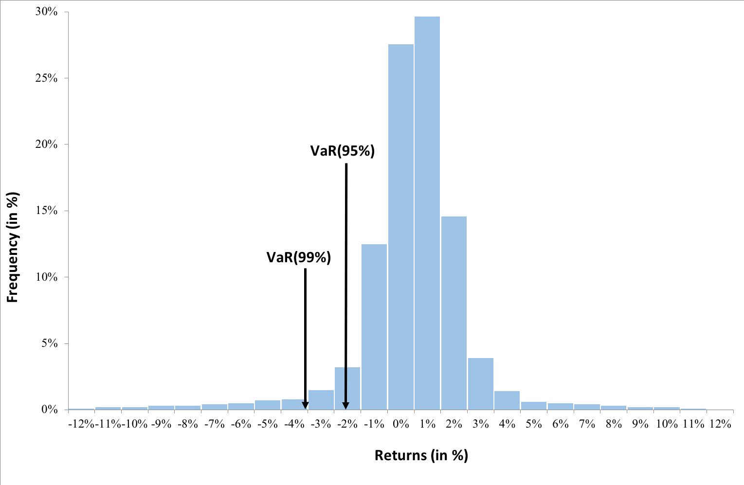
Value at risk (VaR)

VaR is the most extensively used risk measure and essentially refers to the maximum loss that should not be exceeded during a specific period of time with a given probability. VaR is mainly used to calculate minimum capital requirements for institutions that are needed to fulfill their financial obligations, decide limits for asset management and allocation, calculate insurance premiums based on risk and set margin for derivatives transactions.
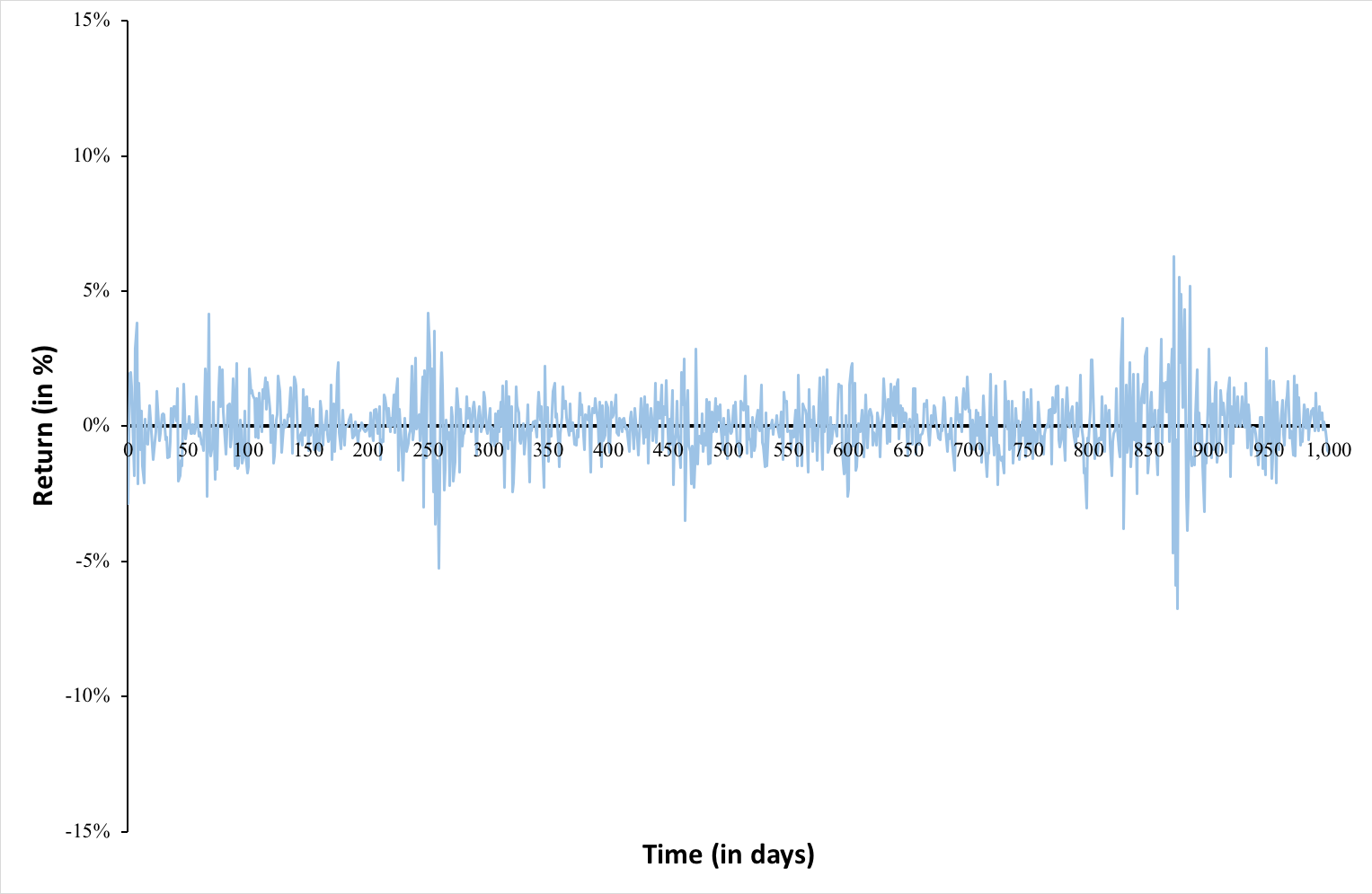
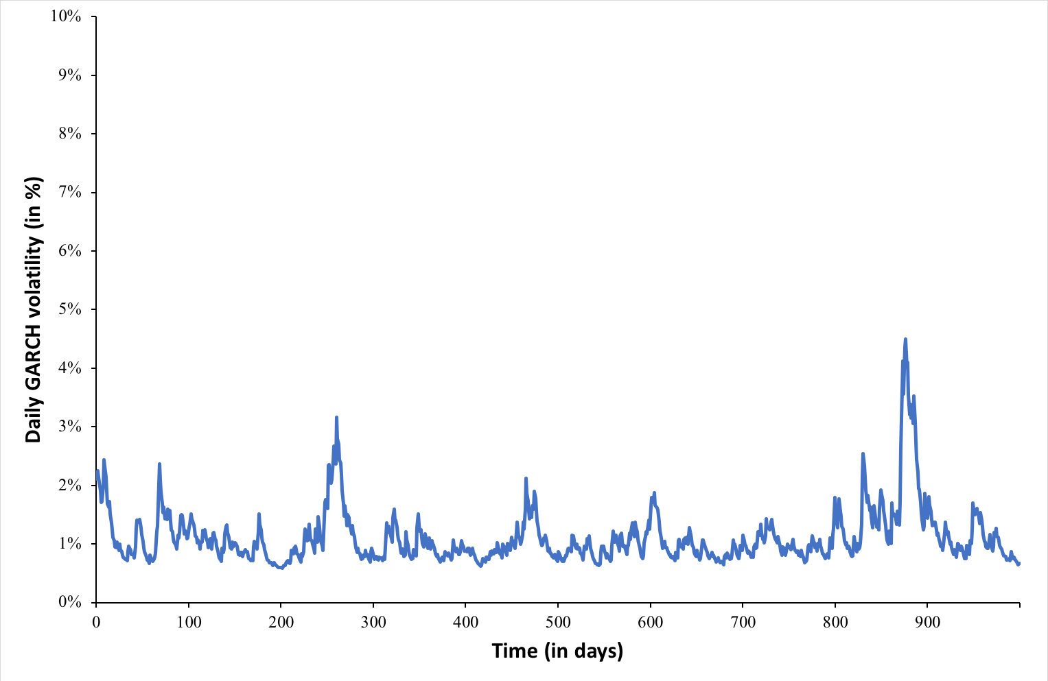
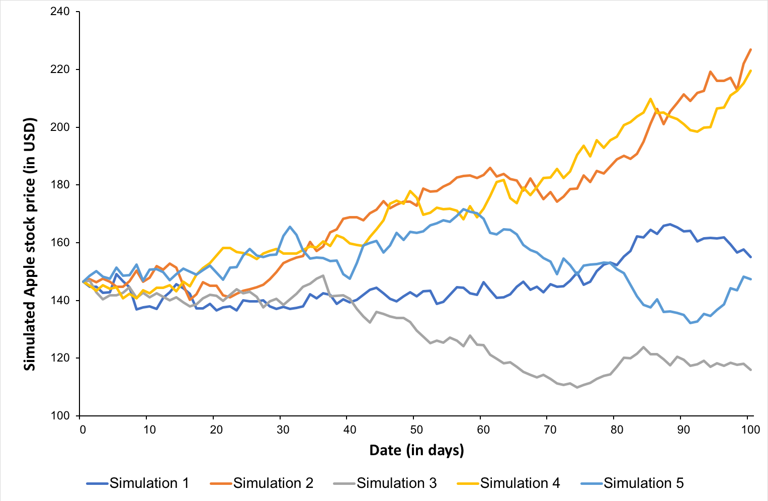
To estimate market risk, we model the statistical distribution of the changes in the market position. Usual models used for the task include normal distribution, the historical distribution and the distributions based on Monte Carlo simulations.

Expected Shortfall

The Expected Shortfall (ES) (also known as Conditional VaR (CVaR), Average Value at risk (AVaR), Expected Tail Loss (ETL) or Beyond the VaR (BVaR)) is a statistic measure used to quantify the market risk of a portfolio. This measure represents the expected loss when it is greater than the value of the VaR calculated with a specific probability level (also known as confidence level).

Credit Risk Measures

Probability of Default (PD) is the probability that a borrower may default on his debt over a period of 1 year. Exposure at Default (EAD) is the expected amount outstanding in case the borrower defaults and Loss given Default (LGD) refers to the amount expected to lose by the lender as a proportion of the EAD. Thus the expected loss in case of default is calculated as PD*EAD*LGD.

Related Posts on the SimTrade blog

   ▶ Jayati WALIA Value at Risk

   ▶ Akshit GUPTA Options

   ▶ Jayati WALIA Black-Scholes-Merton option pricing model

Useful resources

Articles

Longin F. (1996) The asymptotic distribution of extreme stock market returns Journal of Business, 63, 383-408.

Longin F. (2000) From VaR to stress testing : the extreme value approach Journal of Banking and Finance, 24, 1097-1130.

Longin F. and B. Solnik (2001) Extreme correlation of international equity markets Journal of Finance, 56, 651-678.

Books

Embrechts P., C. Klüppelberg and T Mikosch (1997) Modelling Extremal Events for Insurance and Finance.

Embrechts P., R. Frey, McNeil A. J. (2022) Quantitative Risk Management, Princeton University Press.

Gumbel, E. J. (1958) Statistics of extremes. New York: Columbia University Press.

Longin F. (2016) Extreme events in finance: a handbook of extreme value theory and its applications Wiley Editions.
Corporate Finance Institute Basel Accords

Other materials

Extreme Events in Finance

QRM Tutorial

About the author

The article was written in September 2021 by Jayati WALIA (ESSEC Business School, Grande Ecole Program – Master in Management, 2019-2022).