Minimum Volatility Portfolio

January 9, 2023 by Youssef LOURAOUI

In this article, Youssef LOURAOUI (Bayes Business School, MSc. Energy, Trade & Finance, 2021-2022) elaborates on the concept of Minimum Volatility Portfolio, which is derived from Modern Portfolio Theory (MPT) and also in practice to build investment funds.

This article is structured as follows: we introduce the concept of Minimum Volatility Portfolio. Next, we present some interesting academic findings, and we finish by presenting a theoretical example to support the explanations given in this article.

Introduction

The minimum volatility portfolio represents a portfolio of assets with the lowest possible risk for an investor and is located on the far-left side of the efficient frontier. Note that the minimum volatility portfolio is also called the minimum variance portfolio or more precisely the global minimum volatility portfolio (to distinguish it from other optimal portfolios obtained for higher risk levels).

Modern Portfolio Theory’s fundamental notion had significant implications for portfolio construction and asset allocation techniques. In the late 1970s, the portfolio management business attempted to capture the market portfolio return. However, as financial research progressed and some substantial contributions were made, new factor characteristics emerged to capture extra performance. The financial literature has long encouraged taking on more risk to earn a higher return. However, this is a common misconception among investors. While extremely volatile stocks can produce spectacular gains, academic research has repeatedly proved that low-volatility companies provide greater risk-adjusted returns over time. This occurrence is known as the “low volatility anomaly,” and it is for this reason that many long-term investors include low volatility factor strategies in their portfolios. This strategy is consistent with Henry Markowitz’s renowned 1952 article, in which he embraces the merits of asset diversification to form a portfolio with the maximum risk-adjusted return.

Academic Literature

Markowitz is widely regarded as a pioneer in financial economics and finance due to the theoretical implications and practical applications of his work in financial markets. Markowitz received the Nobel Prize in 1990 for his contributions to these fields, which he outlined in his 1952 Journal of Finance article titled “Portfolio Selection.” His seminal work paved the way for what is now commonly known as “Modern Portfolio Theory” (MPT).

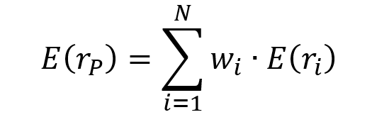
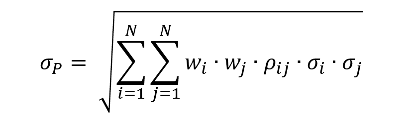
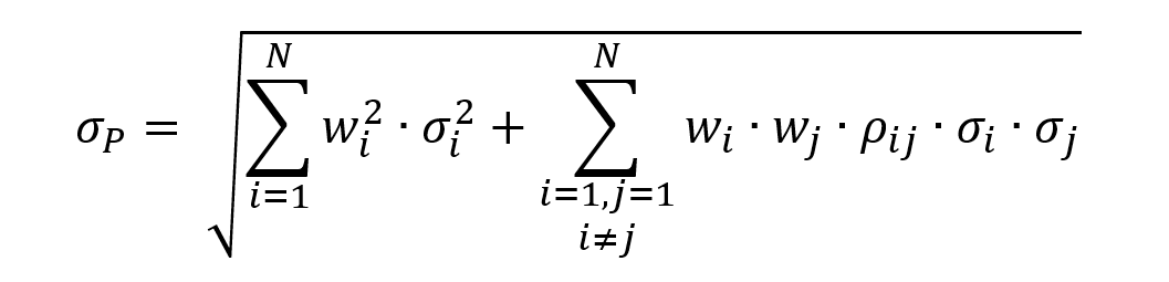
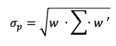
In 1952, Harry Markowitz created modern portfolio theory with his work. Overall, the risk component of MPT may be evaluated using multiple mathematical formulations and managed through the notion of diversification, which requires building a portfolio of assets that exhibits the lowest level of risk for a given level of expected return (or equivalently a portfolio of assets that exhibits the highest level of expected return for a given level of risk). Such portfolios are called efficient portfolios. In order to construct optimal portfolios, the theory makes a number of fundamental assumptions regarding the asset selection behavior of individuals. These are the assumptions (Markowitz, 1952):

The only two elements that influence an investor’s decision are the expected rate of return and the variance. (In other words, investors use Markowitz’s two-parameter model to make decisions.) .
Investors are risk averse. (That is, when faced with two investments with the same expected return but two different risks, investors will favor the one with the lower risk.)
All investors strive to maximize expected return at a given level of risk.
All investors have the same expectations regarding the expected return, variance, and covariances for all hazardous assets. This assumption is known as the homogenous expectations assumption.
All investors have a one-period investment horizon.

Only in theory does the minimum volatility portfolio (MVP) exist. In practice, the MVP can only be estimated retrospectively (ex post) for a particular sample size and return frequency. This means that several minimum volatility portfolios exist, each with the goal of minimizing and reducing future volatility (ex ante). The majority of minimum volatility portfolios have large average exposures to low volatility and low beta stocks (Robeco, 2010).

Example

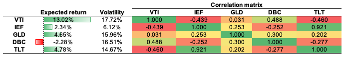
To illustrate the concept of the minimum volatility portfolio, we consider an investment universe composed of three assets with the following characteristics (expected return, volatility and correlation):

Asset 1: Expected return of 10% and volatility of 10%
Asset 2: Expected return of 15% and volatility of 20%
Asset 3: Expected return of 22% and volatility of 35%

Correlation between Asset 1 and Asset 2: 0.30
Correlation between Asset 1 and Asset 3: 0.80
Correlation between Asset 2 and Asset 3: 0.50

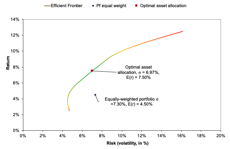
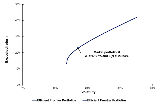
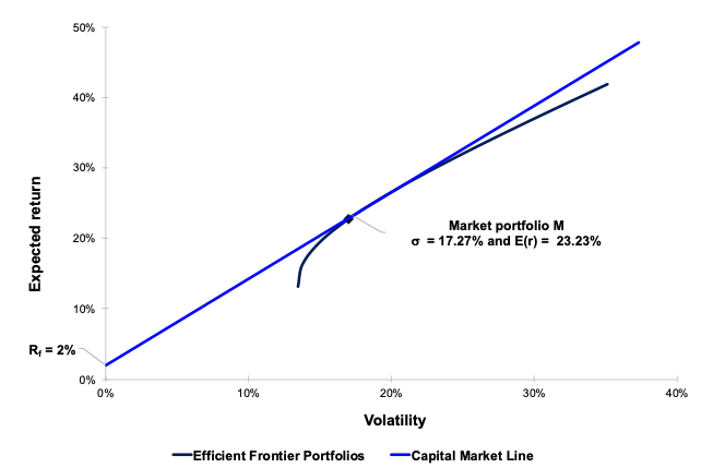
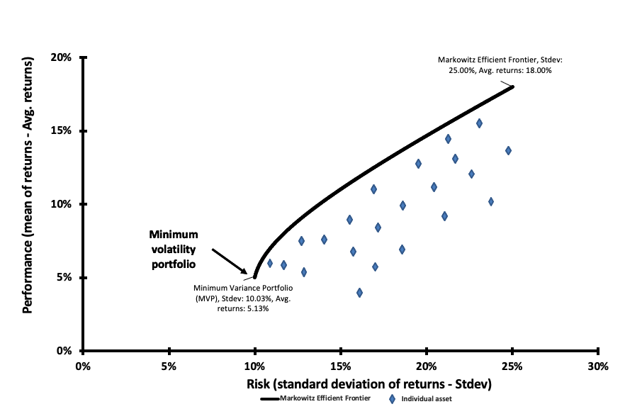
The first step to achieve the minimum variance portfolio is to construct the portfolio efficient frontier. This curve represents all the portfolios that are optimal in the mean-variance sense. After solving the optimization program, we obtain the weights of the optimal portfolios. Figure 1 plots the efficient frontier obtained from this example. As captured by the plot, we can see that the minimum variance portfolio in this three-asset universe is basically concentrated on one holding (100% on Asset 1). In this instance, an investor who wishes to minimize portfolio risk would allocate 100% on Asset 1 since it has the lowest volatility out of the three assets retained in this analysis. The investor would earn an expected return of 10% for a volatility of 10% annualized (Figure 1).

Figure 1. Minimum Volatility Portfolio (MVP) and the Efficient Frontier.

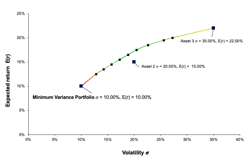
Source: computation by the author.

Excel file to build the Minimum Volatility Portfolio

You can download below an Excel file in order to build the Minimum Volatility portfolio.

Why should I be interested in this post?

Portfolio management’s objective is to optimize the returns on the entire portfolio, not just on one or two stocks. By monitoring and maintaining your investment portfolio, you can accumulate a sizable capital to fulfil a variety of financial objectives, including retirement planning. This article helps to understand the grounding fundamentals behind portfolio construction and investing.

Useful resources

Academic research

Lintner, John. 1965a. Security Prices, Risk, and Maximal Gains from Diversification. Journal of Finance, 20, 587-616.

Lintner, John. 1965b. The Valuation of Risk Assets and the Selection of Risky Investments in Stock Portfolios and Capital Budgets.Review of Economics and Statistics 47, 13-37.

Markowitz, H., 1952. Portfolio Selection. The Journal of Finance, 7, 77-91.

Sharpe, William F. 1963. A Simplified Model for Portfolio Analysis. Management Science, 19, 425-442.

Sharpe, William F. 1964. Capital Asset Prices: A Theory of Market Equilibrium under Conditions of Risk. Journal of Finance, 19, 425-442.

Business analysis

Robeco, 2010 Ten things you should know about minimum volatility investing.

About the author

The article was written in January 2023 by Youssef LOURAOUI (Bayes Business School, MSc. Energy, Trade & Finance, 2021-2022).

Asset allocation techniques

December 19, 2022 by Youssef LOURAOUI

In this article, Youssef LOURAOUI (Bayes Business School, MSc. Energy, Trade & Finance, 2021-2022) presents the concept of asset allocation, a pillar concept in portfolio management.

This article is structured as follows: we introduce the notion of asset allocation, and we use a practical example to illustrate this notion.

Introduction

An investment portfolio is a collection of assets that are owned by an investor. Individual assets, such as bonds and stocks, as well as asset baskets, such as mutual funds or exchange-traded funds, can be employed. When constructing a portfolio, investors often consider both the projected return and risk. A well-balanced portfolio includes a wide range of investments to benefit from diversification.

The asset allocation is one of the processes in the portfolio construction process. At this point, the investor (or fund manager) must divide the available capital into a number of assets that meet the criteria in terms of risk and return trade-off, while adhering to the investment policy, which specifies the amount of exposure an investor can have and the amount of risk the fund manager can hold in his or her portfolio.

The next phase in the process is to evaluate the risk and return characteristics of the various assets. The analyst develops economic and market expectations that can be used to develop a recommended asset allocation for the customer. The distribution of equities, fixed-income securities, and cash; sub asset classes, such as corporate and government bonds; and regional weightings within asset classes are all decisions that must be taken in the portfolio’s asset allocation. Real estate, commodities, hedge funds, and private equity are examples of alternative assets. Economists and market strategists may set the top-down view on economic conditions and broad market movements. The returns on various asset classes are likely to be altered by economic conditions; for example, equities may do well when economic growth has been surprisingly robust whereas bonds may do poorly if inflation soars. These situations will be forecasted by economists and strategists.

The top-down approach

A top-down approach begins with assessment of macroeconomic factors. The investor examines markets and sectors based on the existing and projected economic climate in order to invest in those that are predicted to perform well. Finally, funding is evaluated for specific companies within these categories.

The bottom up approach

A bottom-up approach focuses on company-specific variables such as management quality and business potential rather than economic cycles or industry analysis. It is less concerned with broad economic trends than top-down analysis is, and instead focuses on company particular.

Types of asset allocations

Arnott and Fabozzi (1992) divide asset allocation into three types: 1) policy asset allocation; 2) dynamic asset allocation; and 3) tactical asset allocation.

Policy asset allocation

The policy asset allocation decision is a long-term asset allocation decision in which the investor aims to assess a suitable long-term “normal” asset mix that represents an optimal mixture of controlled risk and enhanced return. The strategies that offer the best prospects of achieving strong long-term returns are inherently risky. The strategies that offer the greatest safety tend to offer very moderate return opportunities. The balancing of these opposing goals is known as policy asset allocation. The asset mix (i.e., the allocation among asset classes) is mechanistically altered in response to changing market conditions in dynamic asset allocation. Once the policy asset allocation has been established, the investor can focus on the possibility of active deviations from the regular asset mix established by policy. Assume the long-run asset mix is established to be 60% equities and 40% bonds. A variation from this mix under certain situations may be tolerated. A decision to diverge from this mix is generally referred to as tactical asset allocation if it is based on rigorous objective measurements of value. Tactical asset allocation does not consist of a single, well-defined strategy.

Dynamic asset allocation

The term “dynamic asset allocation” can refer to both long-term policy decisions and intermediate-term efforts to strategically position the portfolio to benefit from big market swings, as well as aggressive tactical strategies. As an investor’s risk expectations and tolerance for risk fluctuate, the normal or policy asset allocation may change. It is vital to understand what aspect of the asset allocation decision is being discussed and in what context the words “asset allocation” are being used when delving into asset allocation difficulties.

Tactical asset allocation

Tactical asset allocation broadly refers to active strategies that seek to enhance performance by opportunistically adjusting the asset mix of a port- folio in response to the changing patterns of reward available in the capi- tal markets. Notably, tactical asset allocation tends to refer to disciplined techniques for evaluating anticipated rates of return on various asset classes and constructing an asset allocation response intended to capture larger rewards.

Asset allocation application: an example

For this example, lets suppose the fictitious following scenario with real data involved:

Mr. Dubois recently sold his local home construction company in the south of France to a multinational homebuilder with a nationwide reach. He accepted a job as regional manager for that national homebuilder after selling his company. He is now thinking about the financial future for himself and his family. He is looking forward to his new job, where he enjoys his new role and where he will earn enough money to meet his family’s short- and medium-term liquidity demands. He feels strongly that he should not invest the profits of the sale of his company in real estate because his income currently rely on the state of the real estate market. He speaks with a financial adviser at his bank about how to invest his money so that he can retire comfortably in 20 years.

The initial portfolio objective they created seek a nominal return goal of 7% with a Sharpe ratio of at least 1 (for this example, we consider the risk-free rate to be equal to zero). The bank’s asset management division gives Mr Dubois and his adviser with the following data (Figure 1) on market expectations.

Figure 1. Risk, return and correlation estimates on market expectation.
Time-series regression
Source: computation by the author (Data: Refinitiv Eikon).

In order to replicate a global asset allocation approach, we shortlisted a number of trackers that would represent our investment universe. To keep a well-balanced approach, we took trackers that would represent the main asset classes: global equities (VTI – Vanguard Total Stock Market ETF), bonds (IEF – iShares 7-10 Year Treasury Bond ETF and TLT – iShares 20+ Year Treasury Bond ETF) and commodities (DBC – Invesco DB Commodity Index Tracking Fund and GLD – SPDR Gold Shares). To create the optimal asset allocation, we extracted the equivalent of a ten-year timeframe from Refinitiv Eikon to capture the overall performance of the portfolio in the long run. As captured in Figure 1, the global equities was the best performing asset class during the period covered (13.02% annualised return), followed by long term bond (4.78% annualised return) and by gold (4.65% annualised return).

Figure 2. Asset class performance (rebased to 100).
Time-series regression
Source: computation by the author (Data: Refinitiv Eikon).

After analyzing the historical return on the assets retained, as well as their volatility and covariance (and correlation), we can apply Mean-Variance portfolio optimization to determine the optimal portfolio. The optimal asset allocation would be the end outcome of the optimization procedure. The optimal portfolio, according to Markowitz’ seminal study on portfolio construction, will seek to create the best risk-return trade-off for an investor. After performing the calculations, we notice that investing 42.15% in the VTI fund, 30.69% in the IEF fund, 24.88% in the TLT fund, and 2.28% in the GLD fund yields the best asset allocation. As reflected in this asset allocation, the investor intends to invest his assets in a mix of equities (about 43%) and bonds (approximately 55%), with a marginal position (around 3%) in gold, which is widely employed in portfolio management as an asset diversifier due to its correlation with other asset classes. As captured by this asset allocation, we can clearly see the defensive nature of this portfolio, which relies significantly on the bond part of the allocation to operate as a hedge while relying on the equities part as the main driver of returns.

As shown in Figure 3, the optimal asset allocation has a better Sharpe ratio (1.27 vs 0.62) and is captured farther along the efficient frontier line than a naive equally-weighted allocation . The only portfolio with the needed characteristics is the optimal one, as the investor’s goal was to attain a 7% projected return with a minimum Sharpe ratio of 1.

Figure 3. Optimal asset allocation and the Efficient Frontier plot.
Time-series regression
Source: computation by the author (Data: Refinitiv Eikon).

Will this allocation, however, continue to perform well in the future? The market’s reliance on future expectations, return, volatility, and correlation predictions, as well as the market regime, will ultimately determine how much the performance predicted by this study will really change in the future.

Excel file for asset allocation

You can find below the Excel spreadsheet that complements the example above.

Why should I be interested in this post?

The purpose of portfolio management is to maximize (expected) returns on the entire portfolio, not just on one or two stocks for a given level of risk. By monitoring and maintaining your investment portfolio, you can build a substantial amount of wealth for a variety of financial goals, such as retirement planning. This post facilitates comprehension of the fundamentals underlying portfolio construction and investing.

Useful resources

Academic research

Arnott, R. D., and F. J. Fabozzi. 1992. The many dimensions of the asset allocation decision. In Active asset allocation, edited by R. Arnott and F. J. Fabozzi. Chicago: Probus Publishing.

Fabozzi, F.J., 2009. Institutional Investment Management: Equity and Bond Portfolio Strategies and Applications. I (4-6). John Wiley and Sons Edition.

Pamela, D. and Fabozzi, F., 2010. The Basics of Finance: An Introduction to Financial Markets, Business Finance, and Portfolio Management. John Wiley and Sons Edition.

About the author

The article was written in December 2022 by Youssef LOURAOUI (Bayes Business School, MSc. Energy, Trade & Finance, 2021-2022).

Implementing Black-Litterman asset allocation model

March 21, 2022 by Youssef LOURAOUI

In this article, Youssef Louraoui (Bayes Business School, MSc. Energy, Trade & Finance, 2021-2022) presents an implementation of the Black-Litterman model, used to determine the expected return of a portfolio by integrating investor’s views regarding the performance of the underlying assets selected in the investment portfolio.

This article follows the following structure: first, we introduce the Black-Litterman model. We then present the mathematical foundations of this model. We conclude with an explanation of the methodology to build the spreadsheet with the results obtained. You will find in this post an Excel spreadsheet which implement the model.

Introduction

The Black-Litterman asset allocation model, established for the first time in the early 1990’s by Fischer Black and Robert Litterman, is a sophisticated strategy for dealing with unintuitive, highly concentrated, and input-sensitive portfolios. The most likely reason that more portfolio managers do not use the Markowitz model, which maximises return for a given degree of risk, is input sensitivity, a well-documented issue with mean-variance optimization.

The Black-Litterman Model employs a Bayesian technique to integrate an investor’s subjective views of expected returns on one or more assets with the market equilibrium vector (prior distribution) of expected returns to obtain a new, mixed estimate of expected returns. The new vector of returns (the posterior distribution) is a weighted complex average of the investor’s views and market equilibrium.

Mathematical foundation

The idea of the Black Litterman estimates is not to find the optimum portfolio weights as in the Markowitz optimization framework, but instead to find the expected return that would be used as an input to compute the optimum portfolio weights. This approach is referred as reversion portfolio optimization technique. The idea behind is that optimum weights are already observed in the market and captured in the market portfolio. We can approach the reasoning by maximizing the following utility function adjusted to the risk:

img_SimTrade_mathematical_foundation_Black_Litterman_6

w^T = transposed of portfolio weights
Π = Implied equilibrium excess return vector
A = price of risk or risk aversion factor
Σ = variance-covariance matrix

We take the partial derivative of U in terms of weights (w) and we derive the following expression:

img_SimTrade_mathematical_foundation_Black_Litterman_5

By setting the partial derivative equal to zero, we can maximize the utility function in term of weights. The proposed approach in the Black Litterman approach is that instead of seeking the optimal weights, which are incorporated in the market portfolio and thus computable via the market capitalization of the equities in the portfolio, we’ll isolate the Π (implied equilibrium excess return) to obtain the optimal expected returns for the portfolio:

We can deconstruct the Black-Litterman model as

img_SimTrade_mathematical_foundation_Black_Litterman_3

τ= scalar
P = Linking matrix
∑ = Variance-covariance matrix
Π= implied equilibrium excess return
A = Price of risk
w = weight vector
Ω = uncertainty of views

The first term of the formula is introduced in order to respect the constraint that the portfolio weights should be equal to one:

The second term of the formula is to compute a weighted average of the implied equilibrium excess return adjusted to the uncertainty of the returns by the view vector weighted with the uncertainty of views:

The final output E(R) is a vector of return n x 1 that represent the equilibrium returns of the market adjusted to investors views.

Implementation of the Black-Litterman asset allocation model in practice

To model a Black-Litterman portfolio allocation, we obtained a large time series to obtain useful results by downloading the equivalent of 23 years of market data from a data provider (in this example, Bloomberg). We generate the variance-covariance matrix after obtaining all necessary statistical data, which includes the expected return and volatility indicated by the standard deviation of the returns for each stock during the provided period.

The data is derived from the Bloomberg terminal. The first step is to calculate the logarithmic returns and excess returns on the selected assets (returns minus the risk-free rate). After calculating the logarithmic returns on each asset, we can estimate the capital asset pricing model’s returns (CAPM) expected returns. This information will be used to calculate the Black-Litterman expected returns on a comparative basis.

1. The first input for the model is the price of risk A, which represents the risk aversion of investor and is obtained by subtracting the expected return of the market the risk-free rate and divided by the variance of the market:

img_SimTrade_Black_Litterman_formulas_for_spreadsheet_1

E(r_m)= expected market returns
r_f = risk-free rate
σ²_m = variance of market

2. We extract the respective market capitalization of each security to obtain their market weights in the portfolio. Given that our investable universe is made of five stocks, we can retrieve their respective market capitalization and compute the weights of each stock in relation to the sum of total market-capitalization in the portfolio.

img_SimTrade_Black_Litterman_formulas_for_spreadsheet_2

Table 1 depicts the optimal weights obtained from their respective market capitalisation, coupled with the respective expected return and volatility.

Table 1. Asset characteristics of Apple, Amazon, Microsoft, Goldman Sachs, and Pfizer.

img_SimTrade_Black_Litterman_spreadsheet_2

Source: computation by the author.

3. We compute the variance-covariance matrix of logarithmic returns using the data analysis tool pack available in Excel (Table 2).

Table 2. Variance-covariance matrix of asset returns

img_SimTrade_Black_Litterman_spreadsheet_5

Source: computation by the author.

4. We compute the implied equilibrium excess return (Π) as the matrix calculation of the price of risk (A) times the matrix multiplication of the weights computed in step 4 times the variance-covariance matrix computed in step 3.

img_SimTrade_Black_Litterman_formulas_for_spreadsheet_3

Π= implied equilibrium excess return
A = Price of risk
w = weight vector

5. The views are incorporated into the model. To achieve this, we provide three views to include into the model. If there are no views, the values will correspond to the market portfolio. The investment manager’s views for the expected return on certain of the portfolio’s assets regularly diverge from the Implied Equilibrium Return Vector (), which serves as the market-neutral starting point for the Black-Litterman model that quantifies the uncertainty associated with each view. The Black-Litterman Model can be used to depict such views in absolute or relative terms. As an illustration, let us suppose that the real and simulated portfolio will have the same views:

View 1: Apple will outperform Microsoft by .05 percent
View 2: Amazon will outperform Microsoft by .1 percent
View 3: Apple will outperform Amazon by .05 percent

To incorporate the vector Q of views, we create a link matrix P where the rows sum to zero. Figure 3 depicts the workings done in the spreadsheet.

Table 3. Views vector and Link Matrix (P)

img_SimTrade_Black_Litterman_spreadsheet_1

Source: computation by the author.

6. We compute omega to determine the degree of uncertainty associated with the views. While Black-Litterman paper used a value of tau equal to 0.25, an important number of academics went for calculating the tau equal to one. For the sake of simplifying the model, consider tau to be equal to one. This input is obtained by multiplying the Linking matrix by the variance-covariance matrix and transposing the Linking matrix (P).

img_SimTrade_Black_Litterman_formulas_for_spreadsheet_4

τ= scalar
P = Linking matrix
∑ = Variance-covariance matrix

7. We integrate all the values computed previously in the Black-Litterman model. Table 4 depicts the results obtained via the Black-Litterman allocation model.

Table 4. Results of the Black-Litterman allocation

img_SimTrade_Black_Litterman_spreadsheet_4

Source: computation by the author.

We can see that the results converge slightly to those from CAPM. Additionally, we can see that the views are reflected in the Black-Litterman expected returns. As a result, we can determine whether or not each view is satisfied. Indeed, Apple outperforms Amazon and Microsoft, while Amazon outperforms Microsoft.

You can download an Excel file to help you construct a portfolio via the Black-Litterman allocation model.

Why should I be interested in this post?

Modern Portfolio Theory is at the heart of modern finance, shaping the modern investing landscape. MPT has become the cornerstone of current financial theory and practice. MPT’s thesis is that winning the market is difficult and requires diversification and taking higher-than-average risks.

MPT has been around for nearly sixty years and shows no signs of slowing down. His theoretical contributions paved the way for more portfolio theory study. But Markowitz’s portfolio theory is sensitive to and depends on further ‘probabilistic’ expansion. This paper expanded on Markowitz’s previous work by incorporating investor views into the asset allocation process.

Useful resources

Academic research

Black, F. and Litterman, R. 1990. Asset Allocation: Combining Investors Views with Market Equilibrium. Goldman Sachs Fixed Income Research working paper

Black, F. and Litterman, R. 1991. Global Asset Allocation with Equities, Bonds, and Currencies. Goldman Sachs Fixed Income Research working paper

Black, F. and Litterman, R. 1992. Global Portfolio Optimization.Financial Analysts Journal, 28-43.

Idzorek, T.M. 2002. A step-by-step guide to Black-Litterman model. Incorporating user-specified confidence levels. Working Paper, 2-11.

Markowitz, H., 1952. Portfolio Selection. The Journal of Finance, 7(1): 77-91.

About the author

The article was written in Mars 2022 by Youssef LOURAOUI (Bayes Business School, MSc. Energy, Trade & Finance, 2021-2022).

Portfolio

November 26, 2021 by Youssef LOURAOUI

In this article, Youssef LOURAOUI (Bayes Business School, MSc. Energy, Trade & Finance, 2021-2022) elaborates on the concept of portfolio, which is a basic element in asset management.

This article is structured as follows: we introduce the concept of portfolio. We give the basic modelling to define and characterize a portfolio. We then expose the different types of portfolios that investors can rely on to meet their financial goals.

Introduction

An investment portfolio is a collection of assets that an investor owns. These assets can be individual assets such as bonds and stocks or baskets of assets such as mutual funds or exchange-traded funds (ETFs). In a nutshell, this refers to any asset that has the potential to increase in value or generate income. When building a portfolio, investors usually consider the expected return and risk. A well-balanced portfolio includes a variety of investments.

Modelling of portfolios

Portfolio weights

At a point of time, a portfolio is fully defined by the weights (w) of the assets of the universe considered (N assets).

Portfolio weights

The sum of the portfolio weights adds up to one (or 100%):

Sum of the portfolio weights

The weight of a given asset i can be positive (for a long position in the asset), equal to zero (for a neutral position in the asset) or negative (for a short position in the asset):

Asset weight for a long position

Asset weight for a neutral position

Asset weight for a short position

Short selling is the process of selling a security without owning it. By definition, a short sell occurs when an investor borrows a stock, sells it, and then buys it later back to repay the lender.

The equally-weighted portfolio is defined as the portfolio with weights that are evenly distributed across the number of assets held:

Equally-weigthed portfolio

Portfolio return: the case of two assets

Over a given period of time, the returns on assets 1 and 2 are equal to r₁ and r₂. In the two-asset portfolio case, the portfolio return r_P is computed as

Return of a 2-asset portfolio

The expected return of the portfolio E(r_P) is computed as

Expected return of a 2-asset portfolio

The standard deviation of the portfolio return, σ(r_P) is computed as

Standard deviation of a 2-asset portfolio return

where:

σ₁ = standard deviation of asset 1
σ₂ = standard deviation of asset 2
σ_1,2 = covariance of assets 1 and 2
ρ_1,2 = correlation of assets 1 and 2

Investing in asset classes with low or no correlation to one another can help you increase portfolio diversification and reduce portfolio volatility. While diversification cannot guarantee a profit or eliminate the risk of investment loss, the ideal scenario is to have a mix of uncorrelated asset classes in order to reduce overall portfolio volatility and generate more consistent long-term returns. Correlation is depicted mathematically as the division of the covariance between the two assets by the individual standard deviation of the asset. Correlation is a more interpretable metric than covariance because it’s measurable within a defined rank. Correlation is measured between -1 and 1, with a high positive correlation showing that the assets move in tandem, while negative correlation depicts securities that have contrary price movements. The holy grail of investing is to invest in securities that offer a low correlation of the portfolio as a whole.

where:

σ_1,2 = covariance of assets 1 and 2
σ₁ = standard deviation of asset 1
σ₂ = standard deviation of asset 2

Correlation is a more interpretable metric than covariance because it’s measurable within a defined rank. Correlation is measured between -1 and 1, with high positive correlation showing that the assets move in tandem, while negative correlation depicts securities that have contrary price movements. The holy grail of investing is to invest in securities that offer a low correlation of the portfolio as a whole.

You can download an Excel file to help you construct a portfolio and compute the expected return and variance of a two-asset portfolio. Just introduce the inputs in the model and the calculations will be performed automatically. You can even draw the efficient frontier to plot the different combinations of portfolios that optimize the risk-return trade-off (to minimize the risk for a given level of expected return or to maximize the expected return for a given level of risk).

Portfolio return: the case of N assets

Over a given period of time, the return on asset i is equal to r_i. The portfolio return can be computed as

Portfolio return

The expression of the portfolio return is then used to compute two important portfolio characteristics for investors: the expected performance measured by the average return and the risk measured by the standard deviation of returns.

The expected return of the portfolio is given by

Expected portfolio return

Because relying on multiple assets can get extremely computationally heavy, we can refer to the matrix form for more straightforward use. We basically compute the vector of weight with the vector of returns (NB: we have to pay attention to the dimension and to the properties of matrix algebra).

w = weight vector
r = returns vector

The standard deviation of returns of the portfolio is given by the following equivalent formulas:

Standard deviation of portfolio return

w_i = weight of asset i
w_j = weight of asset j
σ_i = standard deviation of asset i
σ_j = standard deviation of asset j
ρ_i,j = correlation of asset i,j

Standard deviation of portfolio return

where:

w_i² = squared weight of asset I
σ_i² = variance of asset i
w_i = weight of asset i
w_j = weight of asset j
σ_i = standard deviation of asset i
σ_j = standard deviation of asset j
ρ_i,j = correlation of asset i,j

We can use the matrix form for a more straightforward application due to the computational burden associated with relying on multiple assets. Essentially, we multiply the vector of weights with the variance-covariance matrix and the transposed weight vector (NB: we must pay attention to the dimension and to the properties of matrix algebra).

w = weight vector
∑ = variance-covariance matrix
w’ = transpose of weight vector

You can get an Excel file that will help you build a portfolio and calculate the expected return and variance of a three-asset portfolio. Simply enter the data into the model, and the calculations will be carried out automatically. You can even use the efficient frontier to plot the various portfolio combinations that best balance risk and reward (to minimize the risk for a given level of expected return or to maximize the expected return for a given level of risk).

Basic principles on portfolio construction

Diversify

Diversification, a core principle of Markowitz’s portfolio selection theory, is a risk-reduction strategy that entails allocating assets among a variety of financial instruments, sectors, and other asset classes (Markowitz, 1952). In more straightforward terms, it refers to the concept “don’t put all your eggs in one basket.” If the basket is dropped, all eggs are shattered; if many baskets are used, the likelihood of all eggs being destroyed is significantly decreased. Diversification may be accomplished by investments in a variety of companies, asset types (e.g., bonds, real estate, etc.), and/or commodities such as gold or oil.

Diversification seeks to enhance returns while minimizing risk by investing in a variety of assets that will react differently to the same event(s). Portfolio diversification methods should include not just diverse stocks inside and outside of the same industry, but also diverse asset classes, such as bonds and commodities. When there is an imperfect connection between assets (lower than one), the diversification effect occurs. It is a critical and successful risk mitigation method since risk mitigation may be accomplished without jeopardizing profits. As a result, any prudent investor who is cautious (or ‘risk averse’) will diversify to a certain extent.

Portfolio Asset Allocation

The term “asset allocation” refers to the proportion of stocks, bonds, and cash in a portfolio. Depending on your investing strategy, you’ll determine the percentage of each asset type in your portfolio to achieve your objectives. As markets fluctuate over time, your asset allocation is likely to go out of balance. For instance, if Tesla’s stock price increases, the percentage of your portfolio allocated to stocks will almost certainly increase as well.

Portfolio Rebalancing

Rebalancing is a term that refers to the act of purchasing and selling assets in order to restore your portfolio’s asset allocation to its original state and avoid disrupting your plan.

Reduce investment costs as much as possible

Commission fees and management costs are significant expenses for investors. This is especially important if you frequently purchase and sell stocks. Consider using a discount brokerage business to make your investment. Clients are charged much lesser fees by these firms. Also, when investing for the long run, it is advisable to avoid making judgments based on short-term market fluctuations. To put it another way, don’t sell your stocks just because they’ve taken a minor downturn in the near term.

Invest on a regular basis

It is critical to invest on a regular basis in order to strengthen your portfolio. This will not only build wealth over time, but it will also develop the habit of investing discipline.

Buying in the future

It’s possible that you have no idea how a new stock will perform when you buy it. To be on the safe side, avoid putting your entire position to a single investment. Start with a little investment in the stock. If the stock’s performance fulfils your expectations, you can gradually increase your investments until you’ve covered your entire position.

Types of portfolio

We detail below the different types of portfolios usually proposed by financial institutions that investors can rely on to meet their financial goals.

Aggressive Portfolio

As the name implies, an aggressive portfolio is one of the most frequent types of portfolio that takes a higher risk in the pursuit of higher returns. Stocks in an aggressive portfolio have a high beta, which means they present more price fluctuations compared to the market. It is critical to manage risk carefully in this type of portfolio. Keeping losses to a minimal and taking profits are crucial to success. It is suitable for a high-risk appetite investor.

Defensive Portfolio

A defensive portfolio is one that consists of stocks with a low beta. The stocks in this portfolio are largely immune to market swings. The goal of this type of portfolio is to reduce the risk of losing the principal. Fixed-income securities typically make up a major component of a defensive portfolio. It is suitable for a low-risk appetite investor.

Income Portfolio

Another typical portfolio type is one that focuses on investments that generate income from dividends (for stocks), interests (for bonds) or rents (for real estate). An income portfolio invests in companies that return a portion of their profits to shareholders, generating positive cash flow. It is critical to remember that the performance of stocks in an income portfolio is influenced by the current economic condition.

Speculative Portfolio

Among all portfolio types, a speculative portfolio has the biggest risk. Speculative investments could be made of different assets that possess inherently higher risks. Stocks from technology and health-care companies that are developing a breakthrough product, junk bonds, distressed investments among others might potentially be included in a speculative portfolio. When establishing a speculative portfolio, investors must exercise caution due to the high risk involved.

Hybrid Portfolio

A hybrid portfolio is one that includes passive investments and offers a lot of flexibility. The cornerstone of a hybrid portfolio is typically made up of blue-chip stocks and high-grade corporate or government bonds. A hybrid portfolio provides diversity across many asset classes while also providing stability by combining stocks and bonds in a predetermined proportion.

Socially Responsible Portfolio

A socially responsible portfolio is based on environmental, social, and governance (ESG) criteria. It allows investors to make money while also doing good for society. Socially responsible or ESG portfolios can be structured for any level of risk or investment aim and can be built for growth or asset preservation. The important thing is that they prefer stocks and bonds that aim to reduce or eliminate environmental impact or promote diversity and equality.

Why should I be interested in this post?

Useful resources

Academic research

Mangram, M.E., 2013. A simplified perspective of the Markowitz Portfolio Theory. Global Journal of Business Research, 7(1): 59-70.

Markowitz, H., 1952. Portfolio Selection. The Journal of Finance, 7(1): 77-91.

Business analysis

Edelweiss, 2021.What is a portfolio?

Forbes, 2021.Investing basics: What is a portfolio?

JP Morgan Asset Management, 2021.Glossary of investment terms: Portfolio

About the author

The article was written in November 2021 by Youssef LOURAOUI (Bayes Business School, MSc. Energy, Trade & Finance, 2021-2022).

Passive Investing

November 21, 2021 by Youssef LOURAOUI

In this article, Youssef LOURAOUI (Bayes Business School, MSc. Energy, Trade & Finance, 2021-2022) elaborates on the concept of passive investing.

This article will offer a concise summary of the academic literature on passive investment. After that, we’ll discuss the fundamental principles of passive investment. The article will finish by establishing a link between passive strategies and the Efficient Market Hypothesis.

Review of academic literature on passive investing

We can retrace the foundations of passive investing to the theory of portfolio construction developed by Harry Markowitz. For his theoretical implications, Markowitz’s work is widely regarded as a pioneer in financial economics and corporate finance. For his contributions to these disciplines, which he developed in his thesis “Portfolio Selection” published in The Journal of Finance in 1952, Markowitz received the Nobel Prize in economics in 1990. His ground-breaking work set the foundation for what is now known as ‘Modern Portfolio Theory’ (MPT).

William Sharpe (1964), John Lintner (1965), and Jan Mossin (1966) separately developed the Capital Asset Pricing Model (CAPM). The CAPM was a huge evolutionary step forward in capital market equilibrium theory because it enabled investors to appropriately value assets in terms of their risk. The asset management industry intended to capture the market portfolio return in the late 1970s, defined as a hypothetical collection of investments that contains every kind of asset available in the investment universe, with each asset weighted in proportion to its overall market participation. A market portfolio’s expected return is the same as the market’s overall expected return. But as financial research evolved and some substantial contributions were made, new factor characteristics emerged to capture some additional performance.

Core principles of passive investing

Positive outlook: The core element of passive investing is that investors can expect the stock market to rise over the long run. A portfolio that mimics the market will appreciate in lockstep with it.

Low cost: A passive strategy has low transaction costs (commissions and market impact) due to its steady approach and absence of frequent trading. While management fees required by funds are unavoidable, most exchange traded funds (ETFs) – the vehicle of choice for passive investors – charge much below 1%.

Diversification: Passive strategies automatically provide investors with a cost-effective method of diversification. This is because index funds diversify their risk by investing in a diverse range of securities from their target benchmarks.

Reduced risk: Diversification almost usually results in lower risk. Investors can also diversify their holdings more within sectors and asset classes by investing in more specialized index funds.

Passive investing and Efficient Market Hypothesis

The Efficient Market Hypothesis (EMH) asserts that markets are efficient, meaning that all information is incorporated into market prices (Fama, 1970). The passive investing strategy is built on the concept of “buy-and-hold,” or keeping an investment position for a lengthy period without worrying about market timing. This latter technique is frequently implemented through the purchase of exchange-traded funds (ETF) that aim to closely match a given benchmark to produce a performance that is comparable to the underlying index or benchmark. The index might be broad-based, such as the S&P500 index in the US equity market for instance, or more specialized, such as an index that monitors a specific sector or geographical zone.

A study from Bloomberg on index funds suggests that passive investments lead 11.6 trillion $ in the US domestic equity-fund market. Passive investing accounts for approximately 54% of the market, owing largely to the growth of funds tracking the S&P 500, the total US stock market, and other broad US indexes. Large-cap stocks in the United States are widely recognized as the world’s most efficient equity market, contributing to passive investing’s dominance. The $6.2 trillion in passive assets represents less than a sixth of the US stock market, which currently has a market capitalization of approximately $40.4 trillion (Bloomberg, 2021).

Figure 1 depicts the historical monthly returns of the S&P500 highlighting the contraction periods in orange. It is considered as a key benchmark that is heavily tracked by passive instruments like Exchange Traded Funds and Mutual Funds. In a two-decade timeframe analysis, the S&P managed to offer an annualised 5.56% return on average coupled with a 15.16% volatility.

Figure 1. S&P500 historical returns (Jan 2000 – November 2021).

Source: Computation by the author (data source: Thomson Reuters).

Estimation of the S&P500 return

You can download an Excel file with data for the S&P500 index returns (used as a representation of the market).

Why should I be interested in this post?

If you are a business school or university undergraduate or graduate student, this content will help you in grasping the concept of passive investing, which is in practice key to investors, and which has attracted a lot of attention in academia.

Useful resources

Academic research

Lintner, J. 1965a. The Valuation of Risk Assets and the Selection of Risky Investments in Stock Portfolios and Capital Budgets. The Review of Economics and Statistics, 47(1): 13-37.

Lintner, J. 1965b. Security Prices, Risk and Maximal Gains from Diversification. The Journal of Finance, 20(4): 587-615.

Mangram, M.E., 2013. A simplified perspective of the Markowitz Portfolio Theory. Global Journal of Business Research, 7(1): 59-70.

Markowitz, H., 1952. Portfolio Selection. The Journal of Finance, 7(1): 77-91.

Mossin, J. 1966. Equilibrium in a Capital Asset Market.Econometrica, 34(4): 768-783.

Sharpe, W.F. 1963. A Simplified Model for Portfolio Analysis.Management Science, 9(2): 277-293.

Sharpe, W.F. 1964. Capital Asset Prices: A theory of Market Equilibrium under Conditions of Risk. The Journal of Finance, 19(3): 425-442.

Business analysis

JP Morgan Asset Management, 2021.Glossary of investment terms: Passive Investing

Bloomberg, 2021. Passive likely overtakes active by 2026, earlier if bear market

About the author

The article was written in November 2021 by Youssef LOURAOUI (Bayes Business School, MSc. Energy, Trade & Finance, 2021-2022).

Alpha

November 20, 2021 by Youssef LOURAOUI

In this article, Youssef LOURAOUI (Bayes Business School, MSc. Energy, Trade & Finance, 2021-2022) elaborates on the concept of alpha, one of the fundamental parameters for portfolio performance measure.

This article is structured as follows: we introduce the concept of alpha in asset management. Next, we present some interesting academic findings on the alpha. We finish by presenting the mathematical foundations of the concept.

Introduction

The alpha (also called Jensen’s alpha) is defined as the additional return delivered by the fund manager on the overall performance of the portfolio compared to the market performance (Jensen, 1968). A key issue in finance (and particularly in portfolio management) has been evaluating the performance of portfolio managers. The term ‘performance’ encompasses at least two independent dimensions (Sharpe, 1967): 1) The portfolio manager’s ability to boost portfolio returns by successful forecasting of future security prices; and 2) The portfolio manager’s ability to minimize (via “efficient” diversification) the amount of “insurable risk” borne by portfolio holders.

The primary hurdle to evaluating a portfolio’s performance in these two categories has been a lack of a solid grasp of the nature and assessment of “risk”. Risk aversion appears to predominate in the capital markets, and as long as investors accurately perceive the “riskiness” of various assets, this indicates that “risky” assets must on average give higher returns than less “risky” assets. Thus, when evaluating portfolios’ performance, the implications of varying degrees of risk on their returns must be considered (Sharpe, 1967).

One way of representing the performance is by linking the performance of a portfolio to the security market line (SML). Figure 1 depicts the relation between the portfolio performance in relation to the security market line. As illustrated in Figure 1 below, Fund A has a negative alpha as it is located under the SML, implying a negative performance of the fund manager compared to the market. Fund B has a positive alpha as it is located above the SML, implying a positive performance of the fund manager compared to the market.

Figure 1. Alpha and the Security Market Line

Source: Computation by the author.

You can download below an Excel file with data to compute Jensen’s alpha for fund performance analysis.

Academic Literature

Jensen develops a risk-adjusted measure of portfolio performance that quantifies the contribution of a manager’s forecasting ability to the fund’s returns. In the first empirical study to assess the outperformance of fund managers, Jensen aimed at quantifying the predictive ability of 115 mutual fund managers from 1945 to 1964. He looked at their ability to produce returns above the expected return given the risk level of each portfolio. Not only does the evidence on mutual fund performance indicate that these 115 funds on average were unable to forecast security prices accurately enough to outperform a buy-and-hold strategy, but there is also very little evidence that any individual fund performed significantly better than what we would expect from mutual random chance. Additionally, it is critical to highlight that these conclusions hold even when fund returns are measured net of management expenses (that is assume their bookkeeping, research, and other expenses except brokerage commissions were obtained free). Thus, on average, the funds did not appear to be profitable enough in their trading activity to cover even their brokerage expenses.

Mathematical derivation of Jensen’s alpha

The portfolio performance metric given below is derived directly from the theoretical results of Sharpe (1964), Lintner (1965a), and Treynor (1965) capital asset pricing models. All three models assume that (1) all investors are risk-averse and single-period expected utility maximizers, (2) all investors have identical decision horizons and homogeneous expectations about investment opportunities, (3) all investors can choose between portfolios solely based on expected returns and variance of returns, (4) all transaction costs and taxes are zero, and (5) all assets are infinitely fungible. With the extra assumption of an equilibrium capital market, each of the three models produces the following equation for the expected one-period return defined by (Jensen, 1968):

E(r): the expected return of the fund
r_f: the risk-free rate
E(r_m): the expected return of the market
β(E(r_m) – r_f): the systematic risk of the portfolio
α: the alpha of the portfolio (Jensen’s alpha)

Why should I be interested in this post?

If you are a business school or university student, this post will help you to understand the fundamentals of investment.

Useful resources

Academic research

Fama, Eugene F. 1965. The Behavior of Stock Market Prices.Journal of Business 37, 34-105.

Fama, Eugene F. 1967. Risk, Return, and General Equilibrium in a Stable Paretian Market. Chicago, IL: University of Chicago.Unpublished manuscript.

Fama, Eugene F. 1968. Risk, Return, and Equilibrium: Some Clarifying Comments. Journal of Finance, 23, 29-40.

Lintner, John. 1965a. Security Prices, Risk, and Maximal Gains from Diversification. Journal of Finance, 20, 587-616.

Lintner, John. 1965b. The Valuation of Risk Assets and the Selection of Risky Investments in Stock Portfolios and Capital Budgets.Review of Economics and Statistics 47, 13-37.

Markowitz, H., 1952. Portfolio Selection. The Journal of Finance, 7, 77-91.

Sharpe, William F. 1963. A Simplified Model for Portfolio Analysis. Management Science, 19, 425-442.

Sharpe, William F. 1964. Capital Asset Prices: A Theory of Market Equilibrium under Conditions of Risk. Journal of Finance, 19, 425-442.

Sharpe, William F. 1966. Mutual Fund Performance. Journal of Business39, Part 2: 119-138.

Treynor, Jack L. 1965. How to Rate Management of Investment Funds.Harvard Business Review 18, 63-75.

Business analysis

JP Morgan Asset Management, 2021.Glossary of investment terms: Alpha

About the author

The article was written in November 2021 by Youssef LOURAOUI (Bayes Business School,, MSc. Energy, Trade & Finance, 2021-2022).

Capital Market Line (CML)

January 30, 2024November 20, 2021 by Youssef LOURAOUI

In this article, Youssef LOURAOUI (Bayes Business School, MSc. Energy, Trade & Finance, 2021-2022) presents the Capital Market Line (CML), a key concept in asset pricing derived from the Capital Asset Pricing Model (CAPM).

This article is structured as follows: we first introduce the concept. We then illustrate how to estimate the capital market line (CML). We finish by presenting the mathematical foundations of the CML.

Capital Market Line

An optimal portfolio is a set of assets that maximizes the trade-off between expected return and risk: for a given level of risk, the portfolio with the highest expected return, or for a given level of expected return, the portfolio with the lowest risk.

Let us consider two cases: 1) when investors have access to risky assets only; 2) when investors have access to risky assets and a risk-free asset (earning a constant interest rate, 2% for example below).

Risky assets

In the case of risky assets only, the efficient frontier (the set of optimal portfolios) is represented below in Figure 1.

Figure 1. Efficient frontier with risky assets only.
img_Simtrade_CML_graph_1
Source: Computation by the author.

Risky assets and a risk-free asset

In the case of risky assets and a risk-free asset, the efficient frontier (the set of optimal portfolios) is represented below in Figure 2. In this case, the efficient frontier is a straight line called the Capital Market Line (CML).

Figure 2. Efficient frontier with risky assets and a risk-free asset.

Source: Computation by the author.

The CML joins the risk-free asset and the tangency portfolio, which is the intersection with the efficient frontier with risky assets only. We can reasonably conclude from Figure 2 that, to increase expected return, an investor has to increase the amount of risk he or she takes to attain returns higher than the risk-free interest rate. As a result, the Sharpe ratio of the market portfolio equals the slope of the CML. If the Sharpe ratio is more than the CML, an investment strategy can be implemented, such as buying assets if the Sharpe ratio is greater than the CML and selling assets if the Sharpe ratio is less than the CML (Drake and Fabozzi, 2011).

Investors who allocate their money between a riskless asset and the risky market portfolio M can expect a return equal to the risk-free rate plus compensation for the number of risk units σ_P) they accept. This result is in line with the underlying notion of all investment theory: investors perform two services in the capital markets for which they might expect to be compensated. First, they enable someone else to utilize their money in exchange for a risk-free interest rate. Second, they face the risk of not receiving the promised returns in exchange for their invested capital. The term E(r_M)- R_f) / σ_M refers to the investor’s expected risk premium per unit of risk, which is also known as the expected compensation per unit of risk taken.

Figure 3 represents the Capital Market Line which connect the risk-free asset to the efficient frontier line. The straight line in Figure 3 represents a combination of a risky portfolio and a riskless asset. Any combination of the risk-free asset and Portfolio A is similarly outperformed by some combination of the risk-free asset and Portfolio B. Continue drawing a line from R_f to the efficient frontier with increasing slopes until you reach Portfolio M’s point of tangency. All other possible portfolio combinations that investors could build are outperformed by the collection of portfolio possibilities along Line R_f-M, which is the CML. The CML, in this sense, represents a new efficient frontier that combines the Markowitz efficient frontier of risky assets with the ability to invest in risk-free securities. The CML’s slope is (E(r_M)- R_f) / σ(_M), which is the highest risk premium compensation that investors can expect for each unit of risk they take on (Reilly and Brown, 2012) (Figure 3).

If we fully invest our cash on the risk-free rate, we would be exactly on the y axis with an expected return of 2%. Each time we move along the curve that connects the risk-free rate to the optimum market portfolio, we allocate less weight to the risk-free rate, and we overweight more on riskier assets (Point A). Points M represents the optimal risky portfolio in the efficient frontier line, which minimizes the overall portfolio variance. It would have a weighting of 45% in stock A and a 55% in stock B, which would offer a 26.23% annualized return for a 17.27% annualized volatility. Point B represents a portfolio composition that is based on a leveraged position of 140% on the optimal risky portfolio and a short position on the risk-free asset of -40% (Figure 3).

Figure 3. Efficient frontier with different points.

Source: Computation by the author.

Mathematical representation

We can define the CML as the line that is tangent to the efficient frontier which connects the risk-free asset with the market portfolio:

img_SimTrade_CML_equations_0

Where:

σ_P: the volatility of portfolio P
R_f: the risk-free interest rate
E(R_M): the expected return of the market M
σ_M: the volatility of the market M
E[R_M– R_f]: the market risk premium.

The expected return of the portfolio can be computed as:

img_SimTrade_CML_equations_1

The Sharpe Ratio is shown in parenthesis, and it compares the performance of an investment, such as a security or portfolio, to the performance of a risk-free asset after adjusting for risk. It is calculated by dividing the difference between the investment returns and the risk-free return by the standard deviation of the investment returns. It denotes the additional amount of return that an investor receives for each unit of risk increase (Sharpe, 1963). We can define it mathematically as:

img_SimTrade_CML_equations_2

We can identify the following relationship between the slope of the CML and the Sharpe ratio of the market portfolio, defined mathematically as follows:

img_SimTrade_CML_equations_3

A simple strategy for stock selection is to buy assets with Sharpe ratios that are higher than the CML and sell those with Sharpe ratios that are lower. Indeed, the efficient market hypothesis implies that beating the market is impossible. As a result, all portfolios should have a Sharpe ratio that is lower than or equal to the market. As a result, if a portfolio (or asset) has a higher Sharpe ratio than the market, this portfolio (or asset) has a higher return per unit of risk (i.e. volatility), which contradicts the efficient market hypothesis. The alpha is the abnormal excess return over the market return at a given level of risk.

Why should I be interested in this post?

Sharpe ratio is a popular tool for assessing portfolio risk/return in finance. The Sharpe ratio informs the investor precisely which portfolio has the best performance among the available options. This simplifies the investor’s decision-making process. The higher the ratio, the greater the return for each unit of risk.

If you are a business school or university undergraduate or graduate student, this content will help you in broadening your knowledge of finance.

Useful resources

Academic research

Pamela, D. and Fabozzi, F., 2010. The Basics of Finance: An Introduction to Financial Markets, Business Finance, and Portfolio Management. John Wiley and Sons Edition.

Lintner, J. 1965a. The Valuation of Risk Assets and the Selection of Risky Investments in Stock Portfolios and Capital Budgets. The Review of Economics and Statistics 47(1): 13-37.

Lintner, J. 1965b. Security Prices, Risk and Maximal Gains from Diversification. The Journal of Finance, 20(4): 587-615.

Mossin, J. 1966. Equilibrium in a Capital Asset Market. Econometrica, 34(4): 768-783.

Reilly, R. K., Brown C. K., 2012. Investment Analysis & Portfolio Management, Tenth Edition.

Sharpe, W.F. 1963. A Simplified Model for Portfolio Analysis. Management Science, 9(2): 277-293.

Sharpe, W.F. 1964. Capital Asset Prices: A Theory of Market Equilibrium under Conditions of Risk. The Journal of Finance, 19(3): 425-442.

About the author

The article was written in November 2021 by Youssef LOURAOUI (Bayes Business School, MSc. Energy, Trade & Finance, 2021-2022).

Smart Beta 1.0

September 23, 2021 by Youssef LOURAOUI

In this article, Youssef LOURAOUI (ESSEC Business School, Global Bachelor of Business Administration, 2017-2021) presents the concept of the smart beta 1.0, the first generation of alternative indexing investment strategies that created a new approach in the asset management industry.

This post is structured as follows: we start by defining smart beta 1.0 as a topic. Finally, we discuss an empirical study by Motson, Clare and Thomas (2017) emphasizing the origin of smart beta.

Definition

The “Smart Beta” expression is commonly used in the asset management industry to describe innovative indexing investment strategies that are alternatives to the market-capitalization-weighted investment strategy (buy-and-hold). In terms of performance, the smart beta “1.0” approach outperforms market-capitalization-based strategies. According to Amenc et al. (2016), the latter have a tendency for concentration and unrewarded risk, which makes them less appealing to investors. In finance, “unrewarded risk” refers to taking on more risk without receiving a return that is commensurate to the increased risk.

When smart beta techniques were first introduced, they attempted to increase portfolio diversification over highly concentrated and capitalization-weighted, as well as to capture the factor premium available in equity markets, such as value indices or fundamentally weighted indices which aim to capture the value premium. While improving capitalization-weighted indices is important, concentrating just on increasing diversity or capturing factor exposure may result in a less than optimal outcome. The reason for this is that diversification-based weighting systems will always result in implicit exposure to certain factors, which may have unintended consequences for investors who are unaware of their implicit factor exposures. Unlike the second generation of Smart Beta, the first generation of Smart Beta are integrated systems that do not distinguish between stock selection and weighting procedures. The investor is therefore required to be exposed to certain systemic risks, which are the source of the investor’s poor performance.

Thus, the first-generation Smart Beta indices are frequently prone to value, small- or midcap, and occasionally contrarian biases, since they deconcentrate cap weighted indices, which are often susceptible to momentum and large growth risk. Furthermore, distinctive biases on risk indicators that are unrelated to deconcentration but important to the factor’s objectives may amplify these biases even further. Indexes that are fundamentally weighted, for example, have a value bias because they apply accounting measures that are linked to the ratios that are used to construct value indexes.

Empirical study: monkeys vs passive mangers

Andrew Clare, Nick Motson, and Steve Thomas assert that even monkey-created portfolios outperform cap-weighted benchmarks in their study (Motson et al., 2017). A lack of variety in cap-weighting is at the foundation of the problem. The endless monkey theory states that a monkey pressing random keys on a typewriter keyboard for an unlimited amount of time will almost definitely type a specific text, such as Shakespeare’s whole works. For 500 businesses, there is an infinite number of portfolio weighting options totaling 100%; some will outperform the market-capitalization-weighted index, while others will underperform. The authors of the study take the company’s ticker symbol and use the following guidelines to create a Scrabble score for each stock:

A, E, I, O, U, L, N, S, T, R – 1 point. D and G both get two points.
B, C, M, P – 3 points ; F, H, V, W, Y – 4 points ; K – 5 points.
J, X – 8 points ; Q, Z – 10 points

The scores of each company’s tickers are then added together and divided by this amount to determine each stock’s weight in the index. As illustrated in Figure 1, the results obtained are astonishing, resulting in a clear outperformance of the randomly generated portfolios compared to the traditional market capitalization index by 1.5% premium overall.

Figure 1. Result of the randomly generated portfolio with the Cass Scrabble as underlying rule compared to market-capitalization portfolio performance.
Scrabble_performance
Source: Motson et al. (2017).

In the same line, the authors produced 500 weights that add up to one using this technique, with a minimum increase of 0.2 percent. The weights are then applied to a universe of 500 equities obtained from Bloomberg in December 2015 (Motson et al., 2017). The performance of the resultant index is then calculated over the next twelve months. This technique was performed ten million times. As illustrated in Figure 2, the results are striking, with smart beta funds outperforming nearly universally in the 10 million simulations run overall, and with significant risk-adjusted return differences (Motson et al., 2017).

Figure 2. 10 million randomly generated portfolios based on a portfolio construction of 500 stocks
Scrabble_performance
Source: Motson et al. (2017).

For performance analysis, the same method was employed, but this time for a billion simulation. This means they constructed one billion 500-stock indexes with weights set at random or as if by a monkey. Figure 9 suggests that the outcome was not accidental. The black line shows the distribution of 1 billion monkeys’ returns in 2016, while the grey line shows the cumulative frequency. 88 percent of the monkeys outperformed the market capitalization benchmark, according to the graph. The luckiest monkey returned 27.2 percent, while the unluckiest monkey returned just 3.83 percent (Motson et al., 2017) (Figure 3).

FFigure 3. Result of one billion randomly simulated portfolios based on a portfolio construction of 500 stocks.
Scrabble_performance
Source: Motson et al. (2017).

Why should I be interested in this post?

If you are a business school or university undergraduate or graduate student, this content will help you in understanding the various evolutions of asset management throughout the last decades and in broadening your knowledge of finance.

If you’re an investor, you’re probably aware that smart beta funds have become a popular topic. Smart beta is a game-changing development that fills a gap in the market for investors: a better return for a reduced risk, net of transaction and administrative costs. These strategies, in a sense, establish a new market. As a result, smart beta is gaining traction and having an impact on asset management.

Useful resources

Academic research

Amenc, N., F., Goltz, F. and Le Sourd, V., 2016. Investor perception about Smart beta ETF. EDHEC Risk Institute working paper.

Amenc, N., F., Goltz, F. and Martinelli, L., 2013. Smart beta 2.0. EDHEC Risk Institute working paper.

Motson, N., Clare, A. & Thomas, S., 2017. Was 2016 the year of the monkey?. Cass Business School research paper.

About the author

The article was written in September 2021 by Youssef LOURAOUI (ESSEC Business School, Global Bachelor of Business Administration, 2017-2021).

Minimum Volatility Factor

September 3, 2021 by Youssef LOURAOUI

Minimum Volatility Factor

In this article, Youssef LOURAOUI (ESSEC Business School, Global Bachelor of Business Administration, 2017-2021) presents the Minimum Volatility Factor, which is based on a risk factor that aims to get exposure to securities with a low volatility profile as measured by beta compared to the market, as well as a low correlation with other assets.

This article is structured as follows: we begin by defining the minimum volatility factor and reviewing academic studies. The MSCI Minimum Volatility Factor Index, which is well used as a benchmark in the asset management industry, is next presented in terms of performance, risk-return trade-off, and behavior during the Covid-19 crisis. We showcase the ETF market for investors looking to profit from the minimum volatility factor.

Definition

In the world of investing, a factor is any aspect that helps explain an asset’s long-term risk and return performance. In the late 1970s, the portfolio management industry’s objective was to capture the market return on a portfolio. As a result of Markowitz and Tobin’s earlier research, William Sharpe, John Lintner, and Jan Mossin independently developed the Capital Asset Pricing Model (CAPM). Because it enabled investors to properly value assets in terms of systematic risk, the CAPM was a significant evolutionary step forward in the theory of capital market equilibrium (Mangram, 2013).

Eugene Fama and Kenneth French, following the CAPM’s original work, developed the Fama-French Three-Factor model in 1993 to solve the CAPM’s inadequacies. It claims that, in addition to the market risk component of the CAPM, two other factors have an effect on the returns on securities and portfolios: market capitalization (called the “size” factor) and the book-to-market ratio (referred to as the “value” factor). Other factor characteristics were developed to capture some additional performance as financial research advanced and significant contributions were made.

Minimum volatility is based on a risk factor that aims to get exposure to securities with a low volatility profile as measured by beta compared to the market, as well as a low correlation with other assets (MSCI Factor research, 2021).

Academic research

In the late 1970s, the portfolio management industry aimed to capture the market portfolio return, but as financial research advanced and certain significant contributions were made, this gave rise to other factor characteristics to capture some additional performance. The financial literature has long advocated for taking on more risk to get a better rate of return. This, however, is a widespread misunderstanding among investors. While extremely volatile equities can deliver spectacular gains, scholarly research has consistently demonstrated that low-volatility companies deliver superior risk-adjusted returns over time. This phenomenon is referred to as the “low volatility anomaly”, and that is why many long-term investors include low volatility factor strategies in their portfolios. This strategy is consistent with Henry Markowitz’s famous 1952 article, in which he preaches the virtues of asset diversification to construct a portfolio that provides the greatest balanced return in a risk-reward framework.

Empirical studies

Figure 1 represents the Markowitz Efficient Frontier, where all the efficient portfolios lie on the upper line. The efficient frontier is a collection of optimum portfolios that provide the highest expected return for a specified level of risk or the lowest risk for a specified level of return. Portfolios that fall below the efficient frontier are suboptimal because they do not provide a sufficient rate of return relative to the degree of risk (Figure 1).

Figure 1. Markowitz Efficient Frontier
Minimum volatility and Markowitz Efficient Frontier
Source: calculations done by the author

Economic interpretation

The term ‘Risk-Reward trade-off’ alludes to Markowitz’s core principle that the riskier an investment, the greater the required potential return. Investors will typically keep a risky investment only if the anticipated return is sufficiently high to compensate them for incurring the risk. Risk is the risk that the actual return on an investment will be less than expected, which is technically defined by standard deviation. A higher standard deviation indicates a greater risk and, thus, a greater potential return. Investors that are willing to take on risk expect to receive a risk premium. The term “risk premium” refers to “the expected return on an investment that is more than the risk-free rate of return”. The greater the risk, the greater the risk premium required by investors.

MSCI Minimum Volatility Factor Index

MSCI Factor Indexes are rules-based, transparent indexes that target equities with favorable factor qualities, as determined by academic discoveries and empirical outcomes, and are designed for easy implementation, replicability, and usage in both standard indexed and active portfolios. The MSCI Minimum Volatility Indexes are created by optimizing a set of sector, country, and factor restrictions to generate an index with the least overall volatility while also maintaining index replicability and investability. The major ways to executing a minimal volatility strategy fall into two categories in terms of methodology: (1) straightforward rank and selection and (2) optimization-based solutions (MSCI Factor research, 2021).

A straightforward technique rates the universe of stocks by anticipated volatility, then picks a subset of the members from the universe and applies a weighting mechanism. The connection between stock returns, which can have a major influence on the overall volatility strategy, is typically ignored in these techniques. While a basic rank and selection technique represents individual stock volatility, optimization-based approaches take into consideration both volatility and correlation effects, or the size and degree to which stocks move in lockstep (MSCI Factor research, 2021).

A naïve unconstrained minimal volatility strategy, on the other hand, has its own set of difficulties, including biases toward certain sectors and nations, undesirable factor exposures, and possibly excessive rebalancing turnover. However, well-designed optimizations with properly defined restrictions may be able to compensate for these flaws. Minimum volatility is classified as a conservative factor, which means that it has tended to benefit from periods of economic contraction. This type of strategy is more concerned with managing volatility than maximizing gains. In this sense, this strategy has produced a premium over the market for long periods, contradicting the principle that investors should not be rewarded with higher risk-adjusted returns for taking less risk than the market (MSCI Factor research, 2021).

The key objective of a minimum volatility strategy is to capture regional and global exposure to potentially less risky stocks. Historically, the MSCI Minimum Volatility Factor Index, for instance, have achieved lower volatility and lower drawdowns (peak-to-trough declines) relative to their factor counterparts during major market downturns (MSCI Factor research, 2021).

Tactical investors have employed MSCI Minimal Volatility Factor Index to decrease risk during market downturns while maintaining equity exposure. The minimum volatility premium was found in the early 1970s by economist Fischer Black coupled with the pioneer work of Portfolio construction of Henry Markowitz in 1952. and built on by others subsequently. After that, according to one idea, investors underpay for low volatility equities because they perceive them to be less lucrative, while overpaying for high volatility equities because they are seen as long-shot prospects for bigger profits. An alternative scholarly argument contends that investors might be overconfident in their abilities to predict the future, and that their views diverge more for high volatility equities, which have fewer predictable outcomes, resulting in increased volatility and poorer returns (MSCI Factor research, 2021).

Performance of the MSCI Minimum Volatility Factor Index

Figure 2 compares the MSCI Minimum Volatility Factor Index’s performance to those of other factors from May 1999 to May 2020. All indices are rebalanced on a 100-point scale to ensure consistency in performance and to facilitate factor comparisons.

Figure 2. Performance of the MSCI Minimum Volatility Factor Index from 1999-2020.

Source: MSCI Factor research, 2021.

With a 1.16% percent yearly return over the MSCI World Index since 1999, the MSCI World Minimum Volatility (USD) Index has consistently provided excess profits over the long run while maintaining a profile of risk among the most conservative of the peer group analysed (MSCI Factor research, 2021).

Risk-return profile of MSCI Minimum Volatility Factor Index

Figure 3 shows the MSCI Minimum Volatility Factor Index compared to other factors over the period May 1999 – May 2020 in terms of risk/reward. The risk-return tradeoff states that the potential return rises with an increase in risk. Individuals connect low levels of uncertainty about future returns with low potential returns, while high levels of uncertainty or risk are associated with large potential returns. According to the risk-tradeoff trade-off, an investor’s money can generate higher returns only if the investor is willing to endure a higher risk of loss (Figure 3).

Figure 3. Risk-return profile of MSCI Minimum Volatility Factor Index compared to a peer group.

Source: MSCI Factor research, 2021.

Behavior of the MSCI Minimum Volatility Factor Index during the Covid-19 crisis

The Covid-19 crisis has not only caused significant social and economic suffering, but it had also an impact on financial markets. To study the behavior of the factors during the Covid-19 crisis, we compute the return of the MSCI Factor indexes during the different stages of the crisis. The MSCI Factor indexes are: value, size, quality, momentum and minimum volatility. Following Pagano et al. (2020) and Hasaj and Sherer (2021), we decompose the Covid-19 crisis into five stages: origin, incubation, outbreak, fever, and treatment. Each stage is described below.

Origin (01/11/2019 – 01/01/2020): the first instances are reported in Wuhan, China.
Incubation (02/01/2020 – 17/01/2020): during this phase, the number of patients began to rise at a faster rate, raising concerns about the disease’s severity.
Outbreak (20/01/2020 – 21/02/2020): the number of cases rose to the point that the World Health Organization (WHO) decided that this illness may pose a major threat to the world’s population, and the pandemic was proclaimed.
Fever (24/02/2020 – 20/03/2020): markets are extremely volatile, owing to government restrictions aimed at flattening the infection curve, with the decision to impose a lockdown in numerous nations as the most notable measures, among others.
Treatment (23/03/2020 – 15/04/2020): most of this turnaround occurs between March and June 2020, which corresponds with the start of good news about the discovery and widespread use of the vaccine.

Table 1 gives the performance of the MSCI factor indexes during the different stages of the Covid-19 crisis. Performance is measured by the return computed on the time-period of each stage, and then annualized for comparison across the different stages. We use data are from Thomson Reuters.

Table 1. Performance of the MSCI factor indexes during the Covid-19 crisis.

Source: computation by the author (Data source: Thomson Reuters).

One conclusion that can be drawn from our research supports the reason for the minimal volatility strategy, namely, to minimize portfolio volatility by keeping limited exposure to highly volatile stocks. In this respect, the Covid-19 pandemic period served as a significant stress test for this strategy, which outperformed the other return factors in the period preceding and following worldwide containment, with a risk-reward trade-off much higher than the average of the chosen factors.

ETFs to capture the Minimum Volatility factor

Let us recall that an Exchange-Traded Fund (ETF) is an investment vehicle that seeks to mirror the performance of a benchmark like an equity index and is traded on a continuous basis during the day like stocks. By investing in ETFs, an investor gains access to a plethora of diversification options through several asset classes (equity, bonds, currency, commodity, real estate, etc.).

Figure 4 gives the overall ETF distribution of the major providers of minimal volatility factor ETFs in terms of asset under management. By examining the market overview for minimal volatility factor investments, we can observe Blackrock ETFs (iShares) dominance, with 78.43% of the overall minimum volatility factor ETF market. This represents roughly 47B$ of the overall minimum volatility market retained for this benchmark.

Figure 4. Minimum Volatility factor ETF market.

Source: etf.com, 2021.

Table 2 gives more detailed information about the biggest minimum volatility factor ETF providers: the asset under management (AUM), expense ratio (ER) and 3-month total return (3-Mo TR) and the segment for the investments.

Table 2. Ranking of the biggest Minimum Volatility ETF providers.
Minimum Volatility factor ETF market actors
Source: etf.com, 2021.

Why should I be interested in this post?

You may have seen the CAPM linked to the market factor in your 101 finance course if you are an undergraduate or graduate student at a business school or university. This article raises awareness of the presence of other additional risk factors.

If you’re an investor, you might want to explore increasing your exposure to the minimum volatility factor to boost your portfolio’s total return.

Useful resources

Academic research

Markowitz, H., 1952. Portfolio Selection. The Journal of Finance, 7(1): 77-91.

Mangram, M.E., 2013. A simplified perspective of the Markowitz Portfolio Theory. Global Journal of Business Research, 7(1): 59-70

Hasaj, M., Sherer, B., 2021. Covid-19 and Smart-Beta: A Case Study on the Role of Sectors. EDHEC-Risk Institute Working Paper.

Pagano, M., Wagner, C., Zechner, J. 2020. Disaster Resilience and Asset Prices, Working paper.

Business analysis

etf.com, 2021. Biggest Minimum Volatility ETF providers.

MSCI Investment Research, 2021. Factor Focus: Volatility.

About the author

The article was written in September 2021 by Youssef LOURAOUI (ESSEC Business School, Global Bachelor of Business Administration, 2017-2021).

Is smart beta really smart?

April 3, 2021 by Youssef LOURAOUI

Is smart beta really smart?

In this article, Youssef LOURAOUI (ESSEC Business School, Global Bachelor of Business Administration, 2017-2021) presents the concept of smart beta used in the asset management industry.

Mutual funds and Exchange traded funds (ETF) based on the smart beta approach have increased in size during the recent years. As Burton Malkiel (2014), we also wonder if the smart beta approach is really smart.

The smart beta industry

Smart beta funds have experienced a significant growth with total assets under management approaching market 620 billion dollar in the U.S. as shown in Figure 1 (Morningstar Reseach, 2017).

Figure 1. Smart Beta Exchange Traded Products growth in the US market (2000-2017).

Source: Morningstar Research (2017).

Traditional approach in portfolio management

The traditional approach to build asset portfolio is to define asset weights based on the market capitalization. The framework of this traditional approach is based on the Capital Asset Pricing Model (CAPM) introduced by the work of Henry Markowitz and William Sharpe in 1964. The CAPM is based on a set of hypotheses about the market structure and investors:

No intermediaries
No constraints (possibility of short selling)
Supply and demand equilibrium
Inexistence of transaction cost
Investors seeks to maximise its portfolio value by optimizing the mean associated with expected returns while minimizing variance associated with risk
Investors are considered as “rational” with a risk averse profile
Investors have access to the information simultaneously in order to execute their investment ideas

Under this framework, Markowitz developed a model relating the expected return of a given asset and its risk:

Relation between expected return and risk

where E(r) represents the expected return of the asset, r_f the risk-free rate, β a measure of the risk of the asset and E(r_m) the expected return of the market.

In this model, the beta (β) parameter is a key parameter and is defined as:

Beta

where Cov(r,r_m) represents the covariance of the asset with the overall market, and σ(r_m)² is the variance of market return.

The beta represents the sensibility of the asset to the fluctuations of the market. This risk measure helps investors to predict the movements of their asset according to the movement of the market overall. It measures the asset volatility in comparison with the systematic risk inherent to the market. Statistically, the beta represents the slope of the line through a regression of data points between the stock returns in comparison to the market returns. It helps investors to explain how the asset moves compared to the market.

More specifically, we can consider the following cases for beta values:

β = 1 indicates a fluctuation between the asset and its benchmark, thus the asset tends to move in a similar rate than the market fluctuations. A passive ETF replicating an index will present a beta close to 1 with its associated index.
0 < β < 1 indicates that the asset moves in a slower rate than market fluctuations. Defensive stocks, stocks that deliver consistent returns without regarding the market state like P&G or Coca Cola in the US, tend to have a beta with the market lower than 1.
β > 1 indicates a more aggressive effect of amplification between the asset price movements with the market movements. Call options tend to have higher betas than their underlying asset.
β = 0 indicates that the asset or portfolio is uncorrelated to the market. Govies, or sovereign debt bonds, tend to have a beta-neutral exposure to the market.
β < 0 indicates an inverse effect of market fluctuation impact in the asset volatility. In this sense, the asset would behave inversely in terms of volatility compared to the market movements. Put options and Gold typically tend to have negative betas.

In order to better monitor the performance of an actively managed fund, active fund managers seek to improve the performance of their fund compared to the market. This additional performance is measured by the “alpha” (Jensen, 1968) defined by:

Alpha Jensen

where E(r) is the average return of the fund over the period studied, r_f the risk-free rate, E(r_m) the expected return of the market, and β×(E(r_m)-r_f) represents the systematic risk of the fund.

Jensen’s alpha (α) represents the abnormal returns of the fund.

The Smart beta approach

The smart beta approach is based on the construction of a portfolio of assets using several different yield enhancement “factors”. BlackRock Investment Solutions (2021) lists the following factors mainly used in the smart beta approach:

Quality, which aims to study the financial environment of the underlying asset.
Volatility which aims to filter assets according to their risk.
Momentum, which aims to identify trends in the selection of assets to be retained by focusing on stocks that have performed strongly in the short term.
Growth is the approach that aims to select securities that have strong return expectations in the medium to long term.
Size which aims to classify according to the size of the assets.
Value that seeks to denote undervalued assets that are close to their fundamental values.

The smart beta approach is opposed to the traditional portfolio approach where a portfolio is constructed using the weights defined by the market capitalization of its assets. The smart beta approach aims to position the portfolio sensitivity or “beta” according to the market environment expectation of the asset manager. For a bull market, the fund manager will select a set of factors to achieve a pronounced exposure of his portfolio. Symmetrically, for a bear market, the fund manager will select another set of factors opting for a beta neutral approach to protect the sensitivity of his portfolio against bear market fluctuations.

Performance and impact factor

S&P Group (2016) studied the performance of different factors (volatility, momentum, quality, value, dividend yield, growth and size) on the S&P500 index for 1994-2014 broken down into sub-sectors (see Table 1). This study finds that each sector is impacted differently by choosing one factor over another. For example, in the energy sector, the strategies of value and growth has led to a positive performance with respectively 1.22% and 2.56%, while in the industrial sector, the strategies of size were the only factor with a positive performance of 1.66%. In practice, there are two approaches: focusing on a single factor or finding a combination of factors that offers the most interesting risk-adjusted return to the investor in view of his/her investment strategy.

Table 1. Sector exposures to smart beta factors (1994-2014).

Source: S&P Research (2014).

S&P Group (2016) also studies the performance of the factors according to the market cycles (bull, bear or recovery markets), business cycles (expansion or contraction) and investor sentiment (neutral, bullish and bearish). The study shows how each factor has been mostly effective for every market condition.

Table 2. Performance of factors according to different market cycles, business cycles and investor sentiment.

Source: S&P Research (2014).

In summary, the following characteristics of the different approaches discussed in this article can be identified:

The CAPM approach aims to give a practical configuration of the relationship between the return of an asset with the market return as well as the return considered as risk-free.
Alpha is an essential metric in the calculation of the portfolio manager’s return in an actively managed fund. In this sense, alpha and CAPM are linked in the fund given the nature of the formulas used.
Smart beta or factor investing follows an approach that straddles the line between active and passive management where the manager of this type of fund will use factors to filter its source of return generation which differs from the common approach based on CAPM reasoning (Fidelity, 2021).
The conductive link of these three reasoning is closely related to the fact that historically the CAPM model has been a pillar in financial theory, the smart beta being a more recent approach that tries to disrupt the codes of the so-called market capitalization based investment by integrating factors to increase the sources of return. Alpha is related to smart beta in the sense that the manager of this type of fund will want to outperform a benchmark and therefore, alpha allows to know the nature of this out-performance of the manager compared to a benchmark.

Is smart beta really smart?

Nevertheless, the vision of this smart beta approach has raised criticisms regarding the relevance of the financial results that this strategy brings to a portfolio’s return. Malkiel (2014) questioned the smartness of smart beta and found that the performance of this new strategy is only the result of chance in the sense that the persistence of performance is dependent in large part on the market configuration.

In his analysis of the performance of the smart ETF fund called FTSE RAFI over the period 2009-2014, he attributed the out-performance to luck. The portfolio allocation was highly exposed to two financial stocks, Citigroup and Bank of America, which accounted for 15% of the portfolio allocation. Note that Citigroup and Bank of America were prosecuted by the American courts for post-crisis financial events and interest rate manipulation operations related to the LIBOR scandal. This smart beta fund outperformed the passive managed US large cap ETF (SPY). Malkiel associated the asset selection of the FTSE RAFI fund with a bet on Bank of America that with another market configuration it could have ended in a sadder way.

Figure 2. FTSE RAFI ETF (orange) compared with its benchmark (FTSE RAFI US 1000) and with SPY ETF (green).

Source: Thomson Reuters Datastream.

We can conclude that the smart beta strategy can allow, as outlined in Blackrock’s research (BlackRock Investment Solutions, 2021), an opportunity to improve portfolio performance while seeking to manage variables such as portfolio out-performance, minimizing its volatility compared to the market or seeking diversification to reduce the risk of the investor’s portfolio. It is an instrument that must be taken judiciously in order to be able to affirm in fine if it is smart in the end, as Malkiel would say.

Useful resources

Academic articles

Malkiel, B. (2014). Is Smart Beta smart? The Journal of Portfolio Management 40, 5: 127-134

El Lamti N. (2017) Are smart beta strategies really smart? HEC Paris.

Business resources

BlackRock Investment Solutions (2021) What is Factor Investing

Fidelity (2021) Smart beta

S&P Global Research (2016) What Is in Your Smart Beta Portfolio? A Fundamental and Macroeconomic Analysis

Morningstar Research (2017) A Global Guide to Strategic-Beta Exchange-Traded Products

Fidelity (2021) Smart beta

About the author

The article in April 2021 was written by Youssef LOURAOUI (ESSEC Business School, Global Bachelor of Business Administration, 2017-2021).

ETFs in a changing asset management industry

February 3, 2021 by Youssef LOURAOUI

ETFs in a changing asset management industry

In this article, Youssef LOURAOUI (ESSEC Business School, Global Bachelor of Business Administration, 2016-2020) talks about his research conducted in the field of investing.

As a way of introduction, ETFs have been captivating investors’ attention in the last 20 years since their creation. This financial innovation has shaped how investors place their capital.

Definition

An ETF can be defined as a financial product that is based on a basket of different assets, to replicate the actual performance of each selected investment. An ETF has more or less the same proportion of the underlying components of the basket, depending on the style of management of the asset manager. ETFs represent nearly 90% of the asset under management of the global Exchange Traded Products (ETP).

History

The first ETF was the Standard and Poor’s Depository Receipts (SPDR) introduced in 1993. It appears to be an optimized product that enables investors to trade it like a stock, with a price that fluctuates during the day (not like mutual funds whose value is known at the end of the day only). The main advantage of ETFs for investors is to diversify their investment with lower fees than buying each underlying asset separately. The most important ETFs in the market are the ones with the lowest expense ratio as it is a crucial point to attract money from investors in the fund.

Types of ETF

ETFs can be segmented in different types according to the asset class, geography, sector, investment style among other criteria. According to Blackrock’s classification (2021), the overall ETF market can be divided into the following classes:

Stock ETFs track a certain stock market index, such as the S&P 500 or NASDAQ.
Bond ETFs offer exposure to a wide selection of fixed income instruments.
Sector and industry ETFs invest in a particular industry such as technology, healthcare, or financials.
Commodity ETFs track the price of a commodity such as oil, gold, or wheat.
Style ETFs are devoted to an investment style or market capitalization focus such as large-cap value or small-cap growth.
Alternative ETFs offer exposure to the alternative asset classes and invest in strategies such as real estate, hedge funds and private equity.
Foreign market ETFs follow non-U.S. markets such as the United Kingdom’s FTSE 100 index or Japan’s Nikkei index.
Actively managed ETFs aim to provide a certain outcome to maximize income or outperform an index, while most ETFs are designed to track an index.

Figure 1. Volume of the ETF market worldwide 2003-2019.

Source: Statista (2021).

Figure 1 represents the volume of the ETF market worldwide over the period 2003-2019. With over 6,970 ETFs globally as of 2019 (Statista, 2021), the ETF industry is growing at an increasing pace, recording a thirty-fold increase in terms of market capitalization in the 17-year timeframe of the analysis. It reflects the growing appetite of investors towards this kind of financial instruments as they offer the opportunity for investors to invest virtually in every asset class, geographical region, sector, theme, and investment style (BlackRock, 2021).

iShares (BlackRock), Xtrackers (DWS) and Lyxor (Société Générale) can also be highlighted as key players of the ETF industry in Europe. As shown in Figure 2, Lyxor (a French player) is ranked 3rd most important player with nearly 9% of the overall European ETF market (Refinitiv insights, 2019). iShares represents nearly eight times the weight of Lyxor, which is slightly above the average of the overall European ETF volume in dollars.

Figure 2. Market share at the promoter level by Assets Under Management (March 31, 2019)

Source: Refinitiv insights (2019).

It goes without saying that the key player worldwide remains BlackRock with nearly 1/3 of the global ETF market capitalization. According to Arte documentary, BlackRock is without a doubt a serious actor of the ETF industry as shown in Figure 2 with an unrivaled market share in the European and global ETF market. With more than 7 trillion of asset under management, BlackRock is the leading powerhouse of the asset management industry.

Benefits of ETF

The main benefits of investing in ETFs is the ability to invest in a diversified and straightforward manner in financial markets by owning a chunk of an index with a single investment. It allows investors to position their wealth in a reference portfolio based on equities, bonds or commodities. It also helps them to create a portfolio that suits their needs or preferences in terms of expected return and risk and also liquidity as ETFs can be bought and sold at any moment of the day. Finally, ETFs also allow investors to implement long/short strategies among others.

Risks

Market risk is an essential component to fully understand the risk of owning an ETF. According to the foundations of the modern portfolio theory (Markowitz, 1952), an asset can be deconstructed into two risk factors: an idiosyncratic risk inherent to the asset and a systematic risk inherent to the market. As an ETF are composed of a basket of different assets, the idiosyncratic risk can be neutralized by the effect of diversification, but the systematic risk, also called the market risk is not neutralized and is still present in the ETF.

In terms of risk, we can mention the volatility risk arising from the underlying assets or index that the ETF tries to replicate. In this sense, when an ETF tries to emulate the performance of the underlying asset, it will also replicate its inherent risk (the systematic and non-systematic risk of the underlying asset). This will have a direct impact on the overall risk-return characteristic of investors’ portfolio.

The second risk, common to all funds and that can have a significant impact on the overall performance, concerns the currency risk when the ETF owned doesn’t use the same currency as the underlying asset. In this sense, when owning an ETF that tracks another asset that is quoted in another currency is inherently, investors bears some currency risk as the fluctuations of the pair of currencies can have a significant impact on the overall performance of the position of the investor.

Liquidity risk arises from the difficulty to buy and sell a security in the market. The more illiquid the market, the wider the spreads to compensate the market maker for the task of connecting buyers and sellers. Liquidity is an important concern when picking an ETF as it can impact the performance of the portfolio overall.

Another risk particular to this instrument, is what is called the tracking error between the ETF value and its benchmark (the index that the ETF tries to replicate). This has a significant impact as, depending on the overall dispersion, the mismatch in terms of valuation between the ETF and the benchmark can impact the returns of investors’ portfolio overall.

Passive management and the concept of efficient market

Most ETFs corresponds to “passive” management as the objective is just to replicate the performance of the underlying assets or the index. Passive management is related to the Efficient Market Hypothesis (EMH), assuming that the market is efficient. Passive fund managers aim to replicate a given benchmark believing that in efficient markets active fund management cannot beat the benchmark on the long term.

Passive fund managers invest their funds by:

Pure replication of the benchmark by investing in each component of the basket (vanilla ETF)
Synthetic reproduction of the benchmark by replicating the basket with derivatives products (like futures contracts).

An important concept is market efficiency (also known as the informational efficiency), which is defined as the ability of the market to incorporate all the available information. Efficient market is a state of the market where information is rationally processed and quickly incorporated in the market price.

It is in the heart of the preoccupations of fund managers and analysts to unfold any efficiency in the market because the degree of efficiency impacts their returns directly (CFA Institute, 2011). Fama (1970) proposed a framework analyzing the degree of efficiency in a market. He distinguishes three forms of market efficiency (weak, semi-strong and strong) which correspond to the degree in which information is incorporated in the prices. Earning consistently abnormal returns based on trading with information is the opposite view of what an efficient market is.

The weak form of market efficiency refers to information composed of past market data (past transaction prices and volumes). In a weakly efficient market, past market information is already included in the current market price, and investors will not be able to distinguish any pattern or prediction of future prices based on past data.
The semi-strong of market efficiency refers to publicly available information. This includes market data (as in the week form) and financial disclosed data (financial accounts published by firms, press articles, reports by financial analysts, etc.). If a market is considered in the semi-strong sense, then it must be in a weak sense as well. In this context, there is no additional gain in determining under or overvalued security as all the public data is already incorporated in the asset price.
The strong of market efficiency refers to all information (both public and private). Markets are strongly efficient when they reflect all the available information at any time in the asset prices.

Useful resources

Academic resources

Fama, E. (1970) “Efficient Capital Markets: A Review of Theory and Empirical Work” Journal of Finance 25(2), 383–417.

Business

Arte documentary (2014) “Ces financiers qui dirigent le monde: BlackRock”.

BlackRock (January 2021) ETF overview.

Refinitiv insights (2019) Concentration of the major players in the European ETF market.

About the author

The article was written in February 2021 by Youssef LOURAOUI (ESSEC Business School, Global Bachelor of Business Administration, 2016-2020).

Introduction

Academic Literature

Example

Excel file to build the Minimum Volatility Portfolio

Why should I be interested in this post?

Related posts on the SimTrade blog

Useful resources

Academic research

Business analysis

About the author

Introduction

The top-down approach

The bottom up approach

Types of asset allocations

Policy asset allocation

Dynamic asset allocation

Tactical asset allocation

Asset allocation application: an example

Excel file for asset allocation

Why should I be interested in this post?

Related posts on the SimTrade blog

Useful resources

Academic research

About the author

Introduction

Mathematical foundation

Implementation of the Black-Litterman asset allocation model in practice

Why should I be interested in this post?

Related posts on the SimTrade blog

Useful resources

Academic research

About the author

Introduction

Modelling of portfolios

Portfolio weights

Portfolio return: the case of two assets

Portfolio return: the case of N assets

Basic principles on portfolio construction

Diversify

Portfolio Asset Allocation

Portfolio Rebalancing

Reduce investment costs as much as possible

Invest on a regular basis

Buying in the future

Types of portfolio

Aggressive Portfolio

Defensive Portfolio

Income Portfolio

Speculative Portfolio

Hybrid Portfolio

Socially Responsible Portfolio

Why should I be interested in this post?

Related posts on the SimTrade blog

Useful resources

Academic research

Business analysis

About the author

Review of academic literature on passive investing

Core principles of passive investing

Passive investing and Efficient Market Hypothesis

Estimation of the S&P500 return

Why should I be interested in this post?

Related posts on the SimTrade blog

Useful resources

Academic research

Business analysis

About the author

Introduction

Academic Literature

Mathematical derivation of Jensen’s alpha

Why should I be interested in this post?

Related posts on the SimTrade blog

Useful resources

Academic research

Business analysis

About the author

Capital Market Line

Risky assets

Risky assets and a risk-free asset

Mathematical representation