Risk Management in the Real-Time Arena

December 4, 2024November 20, 2024 by Vardaan CHAWLA

Risk Management in the Real-Time Arena

In this article, Vardaan CHAWLA (ESSEC Business School, Master in Strategy and Management of International Business (SMIB), 2020-2023) shares a case study on Risk Management in the Real-Time Arena: Navigating the Financial Rapids.

As an individual investor venturing into the dynamic world of financial markets, it’s crucial to understand and implement effective risk management strategies. The following article, explores the key principles and techniques to safeguard your investments and navigate the potential risks.

Financial markets are very dynamic, interesting, and filled with opportunities and risks. Learning to manage risks in the always-changing world of financial markets is crucial. In the following article I discuss the effective methods to manage, navigate, and avoid risk while dealing in financial markets to help you make informed decisions and safeguard your money.

Understanding Your Risk Tolerance

The first principle of effective risk management is self-awareness. Before diving into financial markets one must assess one’s own risk tolerance meaning the amount of losses you are able to manage comfortably.

Ask yourself critical questions:

How much capital can I realistically afford to lose?
How would a significant loss impact my financial well-being?
Am I prone to emotional decision-making during market fluctuations?

After answering these questions you can start making your trading and risk management strategies and techniques. A very aggressive investor will be open to taking a high amount of risk with more potential results while a conservative investor will be the opposite, low risk with less potential returns. One must invest based on their own loss tolerance.

Core Risk Management Strategies

Once you understand your risk tolerance, equip yourself with these key risk management strategies:

Position Sizing: This describes how much capital is devoted to a specific deal. Starting small is a vital notion, particularly for novices. A typical place to start is with 1% to 2% of your entire portfolio for each deal. With a diversified portfolio, you can progressively raise position size as your experience and risk tolerance permits.
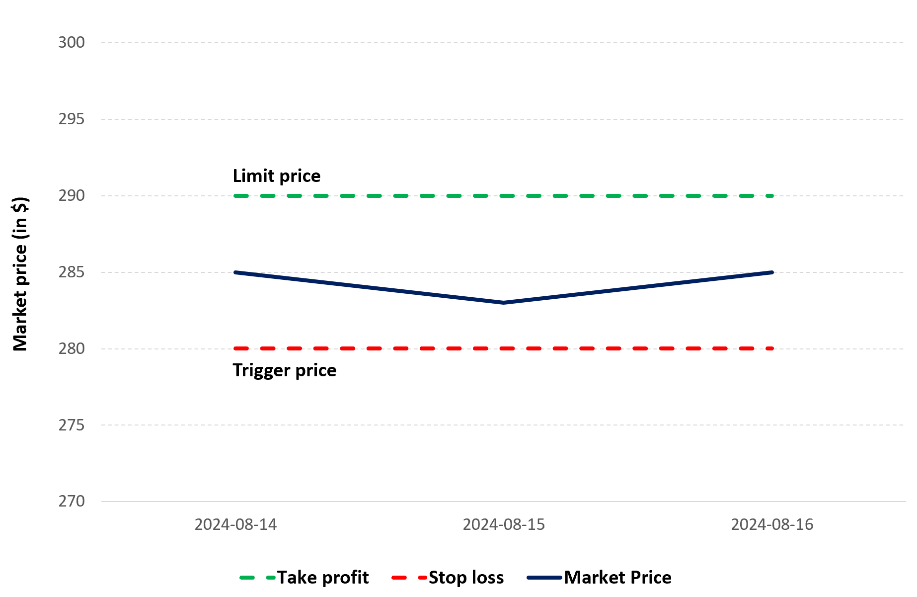
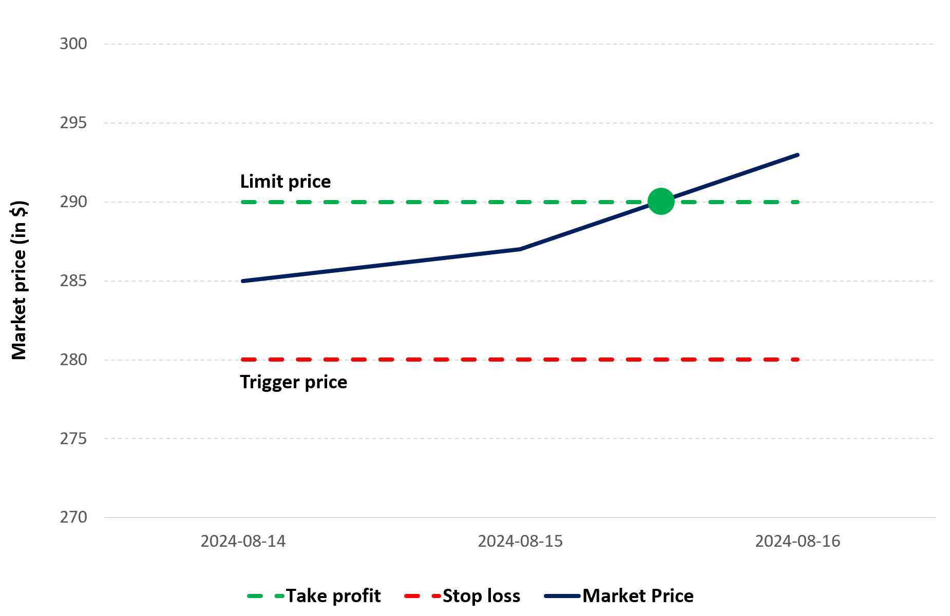
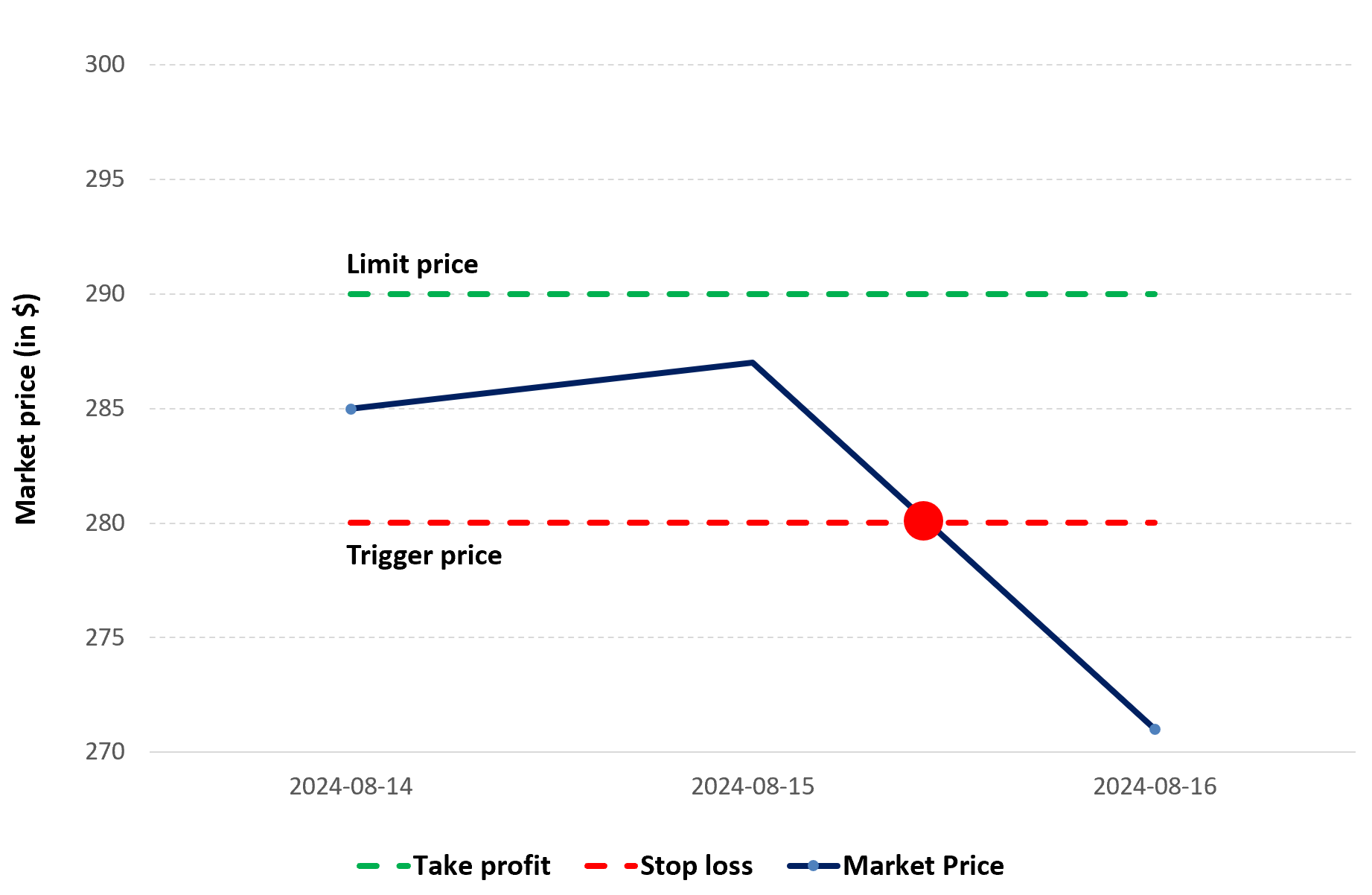
Stop-Loss Orders: These are vital instruments for safeguarding your investment. To limit potential losses if the market swings against your position, a stop-loss order automatically sells an asset when the price hits a predefined level. It’s critical to create stop-loss levels that balance possible asset recovery with risk minimization.
Take Profit Orders: These orders work similarly to stop-loss orders in that they automatically lock in profits by selling an asset when the price hits a predefined level. This lessens the chance of losing gains if the market turns south. To safeguard your earnings and resist the need to cling to a winning position for too long, use take-profit orders wisely.
Diversification: Avoid putting all of your money in one place. Distribute your investments throughout several industries, sectors, and asset classes. This lessens the effect that a fall in one asset will have on the value of your entire portfolio. Diversification makes your portfolio more stable and less vulnerable to changes in the market.
Risk-Reward Ratio: This measure contrasts the possible gain with the possible loss on a certain transaction. Seek for transactions where the possible profit margin outweighs the potential loss margin. A better risk profile is indicated by a greater ratio. Prior to making a trade, evaluating the risk-reward ratio will help you make well-informed judgments regarding potential gain vs downside.

Figure 1. Take profit and stop loss example of Apple stock as on 15th august 2024.
Logo of Talent Carriage
Source: computation by the author.

Advanced Risk Management Techniques

As you gain experience, consider incorporating these advanced techniques:

Hedging: This is the process of offsetting possible losses in your underlying holdings by employing derivative instruments, such as option contracts. Before putting hedging methods into practice, careful thought and comprehension are necessary because they can be complicated.
Volatility Targeting: This strategy modifies the overall risk exposure of your portfolio in response to fluctuations in the market. You may lower the sizes of your positions or devote more capital to less volatile assets during times of high volatility. On the other hand, you may decide to take on larger positions or invest in riskier assets during times of low volatility.

Disciplined Execution: The Key to Success

Risk management is not just about having the right tools; it’s about disciplined execution. Here are some essential practices to cultivate:

Trading Plan: One must work meticulously in developing a comprehensive trading plan that clearly defines your entry, exit, risk management strategies, and what you aim to achieve from trading and avoid emotional and impulsive decision-making.
Monitoring and Adjustment: You must also regularly monitor your portfolio and be updated on financial news in order to prepare for potential future losses or opportunities. To maximize your gains utilize Stop loss orders and take profit orders and adjust your trades and position as and when needed.
Emotional Control: When we receive surprise losses or surprise gains we are inclined to make emotional and impulsive decisions that can lead to further future losses. The trader must always make decisions with a calm composed mind to make sound decisions.

By adopting these risk management principles and maintaining disciplined execution, you can navigate the real-time financial markets with greater confidence and minimize the possibility of significant losses. Remember, risk management is an ongoing process that requires constant evaluation and adaptation.

Useful resources

Justin Kuepper (June 12, 2023) Risk Management Techniques for Active Traders

Amir Samimi & Alireza Bozorgian (September 2021) An Analysis of Risk Management in Financial Markets and Its Effects

About the author

The article was written in November 2024 by Vardaan CHAWLA (ESSEC Business School, Master in Strategy and Management of International Business (SMIB), 2020-2023).

Currency overlay

September 4, 2022 by Jayati WALIA

In this article, Jayati WALIA (ESSEC Business School, Grande Ecole Program – Master in Management, 2019-2022) explains currency overlay which is a mechanism to effectively manage currency risk in asset portfolios.

Overview

Currency risk, also known as exchange-rate risk, forex exchange or FX risk, is a kind of market risk that is caused by the fluctuations in currency exchange rates.

Both individual and institutional investors are diversifying their portfolios through assets in international financial markets, but by doing so they also introduce currency risk in their portfolios.

Consider an investor in the US who decides to invest in the French equity market (say in the CAC 40 index). The investor is now exposed to currency risk due to the movements in EURUSD exchange rate. You can download the Excel file below which illustrates the impact of the EURUSD exchange rate on the overall performance of the investor’s portfolio.

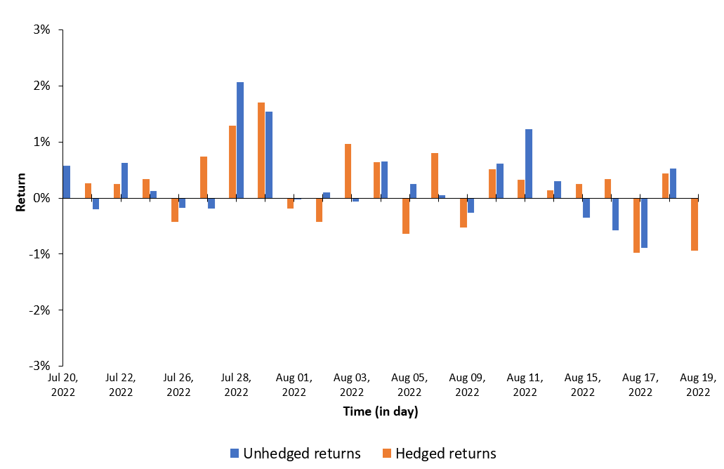
This exercise demonstrates the importance of currency risk in managing an equity portfolio with assets dominated in foreign currencies. We can observe that over a one-month time-period (July 19 – August 19, 2022), the annual volatility of the American investor’s portfolio with FX risk included is 12.96%. On the other hand, if he hedges the FX risk (using a currency overlay strategy), the annual volatility of his portfolio is reduced to 10.45%. Thus, the net gain (or loss) on the portfolio is significantly reliant on the EURUSD exchange-rate.

Figure 1 below represents the hedged an unhedged returns on the CAC 40 index. The difference between the two returns illustrates the currency risk for an unhedged position of an investor in the US on a foreign equity market (the French equity market represented by the CAC 40 index.

Figure 1 Hedged and unhedged returns for a position on the CAC 40 index.
Hedged an unhedged return Source : computation by the author.

Currency overlay is a strategy that is implemented to manage currency exposures by hedging against foreign exchange risk. Currency overlay is typically used by institutional investors like big corporates, asset managers, pension funds, mutual funds, etc. For such investors exchange-rate risk is indeed a concern. Note that institutional investors often outsource the implementation of currency overlays to specialist financial firms (called “overlay managers”) with strong expertise in foreign exchange risk. The asset allocation and the foreign exchange risk management are then separated and done by two different persons (and entities), e.g., the asset manager and the overlay manager. This organization explains the origin of the world “overlay” as the foreign exchange risk management is a distinct layer in the management of the fund.

Overlay managers make use of derivatives like currency forwards, currency swaps, futures and options. The main idea is to offset the currency exposure embedded in the portfolio assets and providing hedged returns from the international securities. The implementation can include hedging all or a proportion of the currency exposure. Currency overlay strategies can be passive or active depending on portfolio-specific objectives, risk-appetite of investors and currency movement viewpoint.

Types of currency overlay strategies

Active currency overlay

Active currency overlay focuses on not just hedging the currency exposure, but also profiting additionally from exchange-rate movements. Investors keeps a part of their portfolio unhedged and take up speculative positions based on their viewpoint regarding the currency trends.

Passive currency overlay

A passive overlay focuses only on hedging the currency exposure to mitigate exchange-rate risk. Passive overlay is implemented through derivative contracts like currency forwards which are used to lock-in a specific exchange-rate for a fixed time-period, thus providing stability to asset values and protection against exchange-rate fluctuations.

Passive overlay is a simple strategy to implement and generally uses standardized contracts, however, it also eliminates the scope of generating any additional profits for the portfolio through exchange-rate fluctuations.

Implementing currency overlays

Base currency and benchmark

Base currency is generally the currency in which the portfolio is dominated or the investor’s domestic currency. A meaningful benchmark selection is also essential to analyze the performance and assess risk of the overlay. World market indices such as those published by MSCI, FTSE, S&P, etc. can be appropriate choices.

Hedge ratio

Establishing a strategic hedge ratio is a fundamental step in implementing a currency overlay strategy. It is the ratio of targeted exposure to be currency hedged by the overlay against the overall portfolio position. Different hedge ratios can have different impact on the portfolio returns and determining the optimal hedge ratio can depend on various factors such as investor risk-appetite and objectives, portfolio assets, benchmark selection, time horizon for hedging etc.

Cost of overlay

The focus of overlays is to hedge the fluctuations in foreign exchange rates by generating cashflows to offset the foreign exchange rate movements through derivatives like currency forwards, currency swaps, futures and options. The use of these derivatives products generates additional costs that impacts the overall performance of the portfolio strategy. These costs must be compared to the benefits of portfolio volatility reduction coming from the overlay implementation.

This cost is also an essential factor in the selection of the hedge ratio.

Note that passive overlays are generally cheaper than active overlays in terms of implementation costs.

Useful resources

Academic articles

Black, F. (1989) Optimising Currency Risk and Reward in International Equity Portfolios. Financial Analysts Journal, 45, 16-22.

Business material

Pensions and Lifetime Savings Association Currency overlay: why and how? video.

About the author

The article was written in September 2022 by Jayati WALIA (ESSEC Business School, Grande Ecole Program – Master in Management, 2019-2022).

The Monte Carlo simulation method for VaR calculation

January 30, 2024March 24, 2022 by Jayati WALIA

In this article, Jayati WALIA (ESSEC Business School, Grande Ecole – Master in Management, 2019-2022) explains the Monte Carlo simulation method for VaR calculation.

Introduction

Monte Carlo simulations are a broad class of computational algorithms that rely majorly on repeated random sampling to obtain numerical results. The underlying concept is to model the multiple possible outcomes of an uncertain event. It is a technique used to understand the impact of risk and uncertainty in prediction and forecasting models.

The Monte Carlo simulation method was invented by John von Neumann (Hungarian-American mathematician and computer scientist) and Stanislaw Ulam (Polish mathematician) during World War II to improve decision making under uncertain conditions. It is named after the popular gambling destination Monte Carlo, located in Monaco and home to many famous casinos. This is because the random outcomes in the Monte Carlo modeling technique can be compared to games like roulette, dice and slot machines. In his autobiography, ‘Adventures of a Mathematician’, Ulam mentions that the method was named in honor of his uncle, who was a gambler.

Calculating VaR using Monte Carlo simulations

The basic concept behind the Monte Carlo approach is to repeatedly run a large number of simulations of a random process for a variable of interest (such as asset returns in finance) covering a wide range of possible scenarios. These variables are drawn from pre-specified probability distributions that are assumed to be known, including the analytical function and its parameters. Thus, Monte Carlo simulations inherently try to recreate the distribution of the return of a position, from which VaR can be computed.

Consider the CAC40 index as our asset of interest for which we will compute the VaR using Monte Carlo simulations.

The first step in the simulation is choosing a stochastic model for the behavior of our random variable (the return on the CAC 40 index in our case).
A common model is the normal distribution; however, in this case, we can easily compute the VaR from the normal distribution itself. The Monte Carlo simulation approach is more relevant when the stochastic model is more complex or when the asset is more complex, leading to difficulties to compute the VaR. For example, if we assume that returns follow a GARCH process, the (unconditional) VaR has to be computed with the Monte Carlo simulation methods. Similarly, if we consider complex financial products like options, the VaR has to be computed with the Monte Carlo simulation methods.

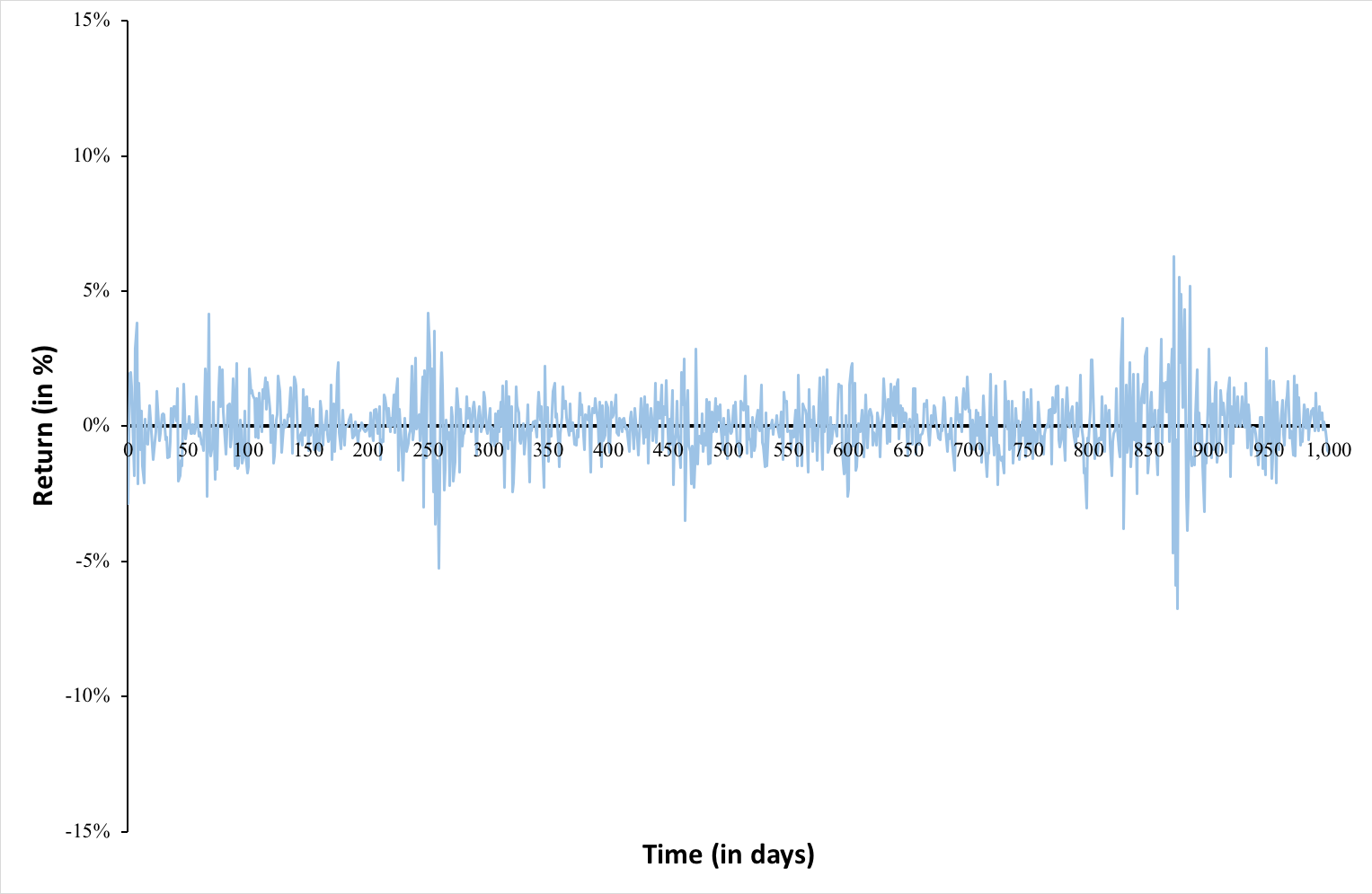
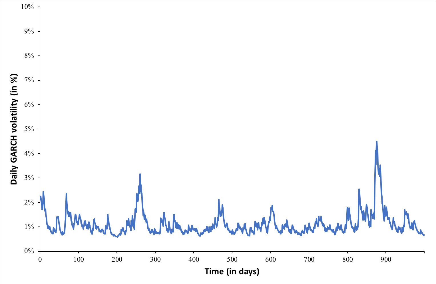
In this post, we compare the Monte Carlo simulation method with the historical method and the variance-covariance method. Thus, we simulate returns for the CAC40 index using the GARCH (1,1) model.
Figure 1 and 2 illustrate the GARCH simulated daily returns and volatility for the CAC40 index.

Figure 1. Simulated GARCH daily returns for the CAC40 index.
img_SimTrade_CAC40_GARCH_ret
Source: computation by the author.

Figure 2. Simulated GARCH daily volatility for the CAC40 index.
img_SimTrade_CAC40_GARCH_vol
Source: computation by the author.

Next, we sort the distribution of simulated returns in ascending order (basically in order of worst to best returns observed over the period). We can now interpret the VaR for the CAC40 index in one-day time horizon based on a selected confidence level (probability).

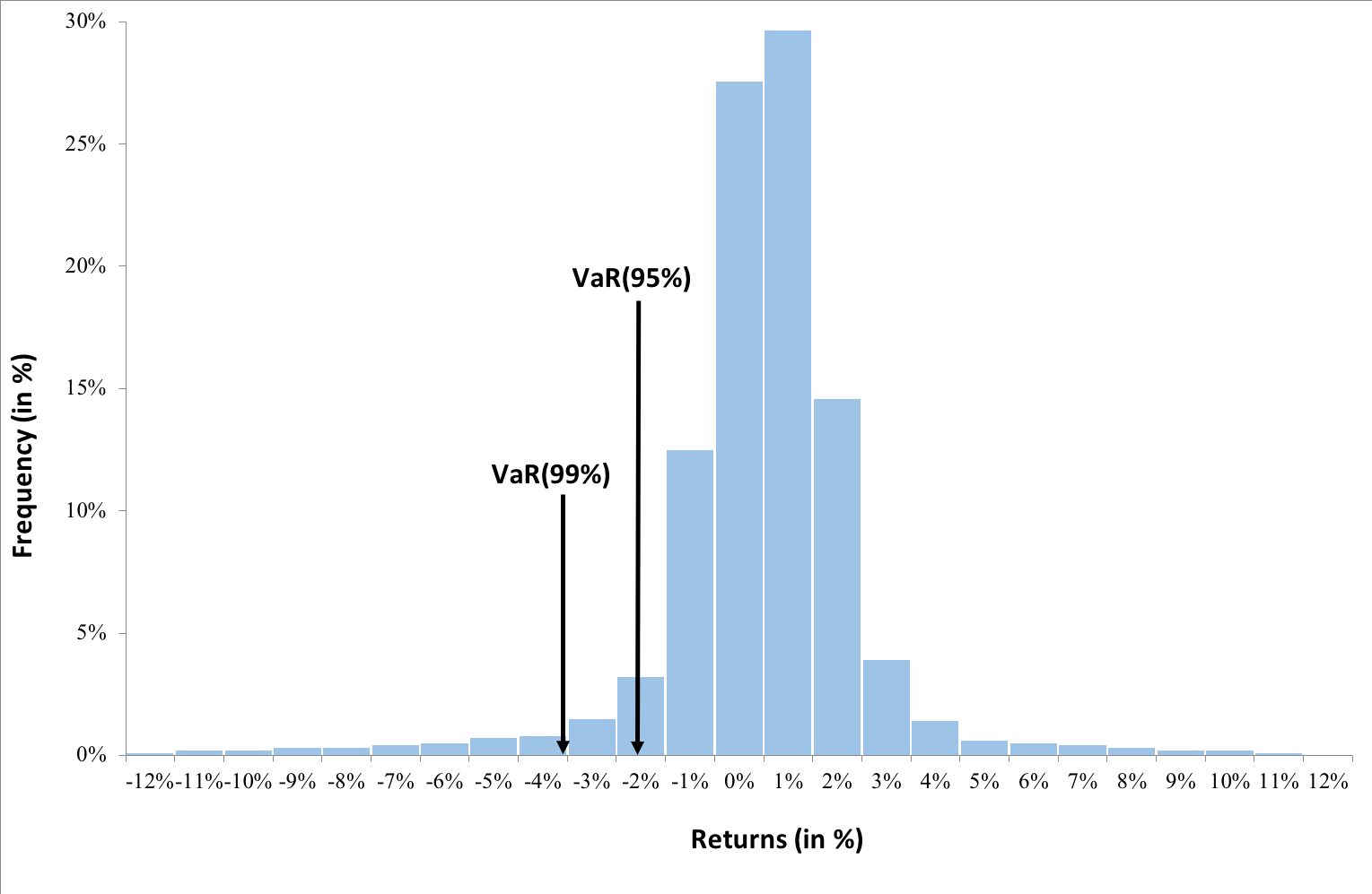
For instance, if we select a confidence level of 99%, then our VaR estimate corresponds to the 1st percentile of the probability distribution of daily returns (the bottom 1% of returns). In other words, there are 99% chances that we will not obtain a loss greater than our VaR estimate (for the 99% confidence level). Similarly, VaR for a 95% confidence level corresponds to bottom 5% of the returns.

Figure 3 below represents the unconditional probability distribution of returns for the CAC40 index assuming a GARCH process for the returns.

Figure 3. Probability distribution of returns for the CAC40 index.
img_SimTrade_CAC40_MonteCarloVaR
Source: computation by the author.

From the above graph, we can interpret VaR for 99% confidence level as -3% i.e., there is a 99% probability that daily returns we obtain in future are greater than -3%. Similarly, VaR for 95% confidence level as -1.72% i.e., there is a 95% probability that daily returns we obtain in future are greater than -1.72%.

You can download below the Excel file for computation of VaR for CAC40 stock using Monte Carlo method involving GARCH(1,1) model for simulation of returns.

Advantages and limitations of Monte Carlo method for VaR

The Monte Carlo method is a very powerful approach to VAR due its flexibility. It can potentially account for a wide range of scenarios. The simulations also account for nonlinear exposures and complex pricing patterns. In principle, the simulations can be extended to longer time horizons, which is essential for risk measurement and to model more complex models of expected returns.

This approach, however, involves investments in intellectual and systems development. It also requires more computing power than simpler methods since the more is the number of simulations generated, the wider is the range of potential scenarios or outcomes modelled and hence, greater would be the potential accuracy of VaR estimate. In practical applications, VaR measures using Monte Carlo simulation often takes hours to run. Time requirements, however, are being reduced significantly by advances in computer software and faster valuation methods.

Useful resources

Jorion P. (2007) Value at Risk, Third Edition, Chapter 12 – Monte Carlo Methods, 321-326.

About the author

The article was written in March 2022 by Jayati WALIA (ESSEC Business School, Grande Ecole Program – Master in Management, 2019-2022).

Quantitative risk management

September 6, 2021 by Jayati WALIA

Quantitative risk management

In this article, Jayati WALIA (ESSEC Business School, Grande Ecole Program – Master in Management, 2019-2022) presents Quantitative risk management.

Introduction

Risk refers to the degree of uncertainty in the future value of an investment or the potential losses that may occur. Risk management forms an integral part of any financial institution to safeguard the investments against different risks. The key question that forms the backbone for any risk management strategy is the degree of variability in the profit and loss statement for any investment.

The process of the risk management has three major phases. The first phase is risk identification which mainly focuses on identifying the risk factors to which the institution is exposed. This is followed by risk measurement that can be based on different types of metrics, from monitoring of open positions to using statistical models and Value-at-Risk. Finally, in the third phase risk management is performed by setting risk limits based on the determined risk appetite, back testing (testing the quality of the models on the historical data) and stress testing (assessing the impact of severe but still plausible adverse scenarios).

Different types of risks

There are several types of risks inherent in any investment. They can be categorized in the following ways:

Market risk

An institution can invest in a broad list of financial products including stocks, bonds, currencies, commodities, derivatives, and interest rate swaps. Market risk essentially refers to the risk arising from the fluctuation in the market prices of these assets that an institution trades or invests in. The changes in prices of these underlying assets due to market volatility can cause financial losses and hence, to analyze and hedge against this risk, institutions must constantly monitor the performance of the assets. After measuring the risk, they must also implement necessary measures to mitigate these risks to protect the institution’s capital. Several types of market risks include interest rate risk, equity risk, currency risk, credit spread risk etc.

Credit risk

The risk of not receiving promised repayments due to the counterparty failing to meet its obligations is essentially credit risk. The counterparty risk can arise from changes in the credit rating of the issuer or the client or a default on a due obligation. The default risk can arise from non-payments on any loans offered to the institution’s clients or partners. After the financial crisis of 2008-09, the importance of measuring and mitigating credit risks has increased many folds since the crisis was mainly caused by defaults on payments on sub-prime mortgages.

Operational risk

The risk of financial losses resulting from failed or faulty internal processes, people (human error or fraud) or system, or from external events like fraud, natural calamities, terrorism etc. refers to operational risk. Operational risks are generally difficult to measure and may cause potentially high impacts that cannot be anticipated.

Liquidity risk

The liquidity risk comprises to 2 types namely, market liquidity risk and funding liquidity risk. In market liquidity risk can arise from lack of marketability of an underlying asset i.e., the assets are comparatively illiquid or difficult to sell given a low market demand. Funding liquidity risk on the other hand refers to the ease with which institutions can raise funding and thus institutions must ensure that they can raise and retain debt capital to meet the margin or collateral calls on their leveraged positions.

Strategic risk

Strategic risks can arise from a poor strategic business decisions and include legal risk, reputational risk and systematic and model risks.

Basel Committee on Banking Supervision

The Basel Committee on Banking Supervision (BCBS) was formed in 1974 by central bankers from the G10 countries. The committee is headquartered in the office of the Bank for International Settlements (BIS) in Basel, Switzerland. BCBS is the primary global standard setter for the prudential regulation of banks and provides a forum for regular cooperation on banking supervisory matters. Its 45 members comprise central banks and bank supervisors from 28 jurisdictions. Member countries include Australia, Belgium, Canada, Brazil, China, France, Hong Kong, Italy, Germany, India, Korea, the United States, the United Kingdom, Luxembourg, Japan, Russia, Switzerland, Netherlands, Singapore, South Africa among many others.

Over the years, BCBS has developed influential policy recommendations concerning international banking and financial regulations in order to exercise judicious corporate governance and risk management (especially market, credit and operational risks), known as the Basel Accords. The key function of Basel accords is to manage banks’ capital requirements and ensure they hold enough cash reserves to meet their respective financial obligations and henceforth survive in any financial and/or economic distress.

Over the years, the following versions of the Basel accords have been released in order to enhance international banking regulatory frameworks and improve the sector’s ability to manage with financial distress, improve risk management and promote transparency:

Basel I

The first of the Basel accords, Basel I (also known as Basel Capital Accord) was developed in 1988 and implemented in the G10 countries by 1992. The regulations intended to improve the stability of the financial institutions by setting minimum capital reserve requirements for international banks and provided a framework for managing of credit risk through the risk-weighting of different assets which was also used for assessing banks’ credit worthiness.
However, there were many limitations to this accord, one of which being that Basel I only focused on credit risk ignoring other risk types like market risk, operational risk, strategic risk, macroeconomic conditions etc. that were not covered by the regulations. Also, the requirements posed by the accord were nearly the same for all banks, no matter what the bank’s risk level and activity type.

Basel II

Basel II regulations were developed in 2004 as an extension of Basel I, with a more comprehensive risk management framework and thereby including standardized measures for managing credit, operational and market risks. Basel II strengthened corporate supervisory mechanisms and market transparency by developing disclosure requirements for international regulations inducing market discipline.

Basel III

After the 2008 Financial Crisis, it was perceived by the BCBS that the Basel regulations still needed to be strengthened in areas like more efficient coverage of banks’ risk exposures and quality and measure of the regulatory capital corresponding to banks’ risks.
Basel III intends to correct the miscalculations of risk that were believed to have contributed to the crisis by requiring banks to hold higher percentages of their assets in more liquid instruments and get funding through more equity than debt. Basel III thus tries to strengthen resilience and reduce the risk of system-wide financial shocks and prevent future economic credit events. The Basel III regulations were introduced in 2009 and the implementation deadline was initially set for 2015 however, due to conflicting negotiations it has been repeatedly postponed and currently set to January 1, 2022.

Risk Measures

Efficient risk measurement based on relevant risk measures is a fundamental pillar of the risk management. The following are common measures used by institutions to facilitate quantitative risk management:

Value at risk (VaR)

VaR is the most extensively used risk measure and essentially refers to the maximum loss that should not be exceeded during a specific period of time with a given probability. VaR is mainly used to calculate minimum capital requirements for institutions that are needed to fulfill their financial obligations, decide limits for asset management and allocation, calculate insurance premiums based on risk and set margin for derivatives transactions.
To estimate market risk, we model the statistical distribution of the changes in the market position. Usual models used for the task include normal distribution, the historical distribution and the distributions based on Monte Carlo simulations.

Expected Shortfall

The Expected Shortfall (ES) (also known as Conditional VaR (CVaR), Average Value at risk (AVaR), Expected Tail Loss (ETL) or Beyond the VaR (BVaR)) is a statistic measure used to quantify the market risk of a portfolio. This measure represents the expected loss when it is greater than the value of the VaR calculated with a specific probability level (also known as confidence level).

Credit Risk Measures

Probability of Default (PD) is the probability that a borrower may default on his debt over a period of 1 year. Exposure at Default (EAD) is the expected amount outstanding in case the borrower defaults and Loss given Default (LGD) refers to the amount expected to lose by the lender as a proportion of the EAD. Thus the expected loss in case of default is calculated as PD*EAD*LGD.

Useful resources

Articles

Longin F. (1996) The asymptotic distribution of extreme stock market returns Journal of Business, 63, 383-408.

Longin F. (2000) From VaR to stress testing : the extreme value approach Journal of Banking and Finance, 24, 1097-1130.

Longin F. and B. Solnik (2001) Extreme correlation of international equity markets Journal of Finance, 56, 651-678.

Books

Embrechts P., C. Klüppelberg and T Mikosch (1997) Modelling Extremal Events for Insurance and Finance.

Embrechts P., R. Frey, McNeil A. J. (2022) Quantitative Risk Management, Princeton University Press.

Gumbel, E. J. (1958) Statistics of extremes. New York: Columbia University Press.

Longin F. (2016) Extreme events in finance: a handbook of extreme value theory and its applications Wiley Editions.
Corporate Finance Institute Basel Accords

Other materials

Extreme Events in Finance

QRM Tutorial

About the author

The article was written in September 2021 by Jayati WALIA (ESSEC Business School, Grande Ecole Program – Master in Management, 2019-2022).

My experience as a portfolio manager in a central bank

November 29, 2020 by Youssef LOURAOUI

My experience as a portfolio manager in a central bank

During my studies at ESSEC Business School, I had the chance to attend the SimTrade course. This course helped me to secure an internship as a risk manager at Bank Al-Maghrib (the central bank of Morocco) as I was asked during my interviews technical questions about financial markets that were covered during the course.

In this article, Youssef LOURAOUI (ESSEC Business School, Global Bachelor of Business Administration, 2020) shares his experience as an intern in the risk management department (middle office) at the Central Bank of Morocco (Bank Al-Maghrib) in 2020.

Bank Al-Maghrib

The central bank of Morocco was founded in 1959 after Morocco proclaimed its independence. It is a 100% state-owned bank that regulates the markets and the economy by implementing monetary and economic policies to ensure the welfare in terms of the parity of prices and the control of inflation. Inflation is a major economic indicator that possesses strategic importance and is part of the major focus for the central bank.

Bank Al-Maghrib

I describe below my experience at Bank Al-Maghrib.

My internship at Bank Al-Maghrib

I was affected at the middle office department, which is in charge of measuring risk exposures and profits and losses on the positions taken by the bank on an investment portfolio of 27,4 billion euros of foreign reserve. One of the key risk exposure metrics is volatility measured by the standard deviation statistically defined as the dispersion of a random variable (asset prices or returns in my case) from its expected value. The standard deviation indicates how much the current return is deviating from its expected historical returns. It is one of the most widely used metrics for investors when analyzing the risk of an investment. Among other key exposures metric, there is what it is called the VaR (Value at Risk) at 99% and a 95% confidence level for 1-day and 30-day positions. In other words, the VaR is a metric used to compute how much loss can the portfolio incur at a % degree of confidence for a given time horizon.

Every day, the Head of the Middle Office organizes a general meeting where he talks about global debriefing of the main financial news that happened overnight and debriefing the middle office desk for the “watch out” assets that could have a potential investment opportunity. Accordingly, the team has also the task of staying in line with the investment decision that characterizes the organization, as it does not operate as an investment banking corporation nor a hedge fund in the risk and leverage used. As the central bank has the special task of keeping safe the national reserve and searching for a good mix to invest in a low risk asset (AAA bonds from European countries coupled with American treasury bonds).

My task aimed to get a hand on the investment mechanism in the middle office of the bank. The investment mechanism consists of the division of the overall portfolio into three main tranches where each one has its characteristics. The first tranche (called also the security tranche) is calculated by analyzing the national need for a currency that needs to be kept safe to establish welfare on the exchange market (based mainly on short term position in low-risk profile asset (Liquid and high rated bonds). The second tranche is based on buy and hold and a market strategy. The first one consists of taking a long position on more risky assets than the first tranche till maturity, there is no selling during the lifetime of the asset (riskier bonds and gold). The second strategy is based on buying and selling liquid assets for an expectation of yielding higher returns.

During my time at the middle office desk, I’ve managed to develop a tool to represent the investment mechanism used for asset allocation. The tool, developed in an Excel spreadsheet, is an intuitive and simplified model that enables the understanding of the investment mechanism. Indeed, it is capable of continuously refreshing the data by importing the most recent quotations (from data providers like Bloomberg or Reuters as the two main financial data providers) to allow for an update of the different exposures and thus allow to respect the proportions of portfolio allocations. It has also a dynamic risk management tool to effectively compute draw-downs (a peak-to-trough decline during a specific period for an investment) and stressed conditions, as I experienced how the markets reacted to the novel Covid-19 pandemic with one of the most historic market movements in a long time.

Some of the key learning outcomes:

The introduction to data analysis by manipulating large datasets

Portfolio optimization based on the Markowitz efficient frontier

Dynamic portfolio allocation based on the fundamentals of the modern portfolio theory

The theory of efficient markets to understand how the markets evolve and move in a different direction as a reaction to events.

Front office, middle office and back office

My internship was also a good opportunity to discover the different departments of the bank: the front office, the middle office, and the back office:

The front office directly deals with the individual or corporate clients of the bank. Salespeople propose adequate products and solutions to the clients (they are in front of them!). Traders intervene in the financial markets on behalf of the clients or for the bank itself (proprietary trading). To answer the demand of clients, financial engineers and quants also develop new products and the associated mathematical models to price them. One of the main trends that are emerging in the front office is the automatization with the help of AI and algorithmic trading that is taken some room in the trading desks. At this time the bank didn’t implement any technology based on high-frequency trading, but it is taking the financial industry by surprise and it goes a long way back, nearly decades ago since the first usage of algorithmic trading.

The middle office situated between the front office and the back office (somewhere in the middle!) deals with the risk management of the bank. Risk managers control the traders’ positions (respect of constraints such as value-at-risk limits and stress tests) and compute the profits and losses (P&L) on traders’ positions daily.

The back-office deals with the conformity and the security check of every trade to ensure a proper settlement.

Note that the frontiers between the front, middle, and back-office may change from one bank to another. And last but not the least, the IT people are also supporting all three departments to make the whole system work. In other words, they are in charge of the maintenance of the technical infrastructure that the bank uses daily to operate fluently, as all the departments are dependent on internal software to intermediate and operate in the market or to communicate between each department of the bank or with another organization. The IT desk has great importance in offering a flawless experience for the employees when using the internal electronic infrastructure. There is the backbone of the bank skeleton.

All in all, the SimTrade module served me well as I managed to gain quickly the necessary knowledge and bridge the gap that I had to be in the best position to achieve the missions I’ve been affected. I especially used the content of Period 2 of the SimTrade certificate, which deals with market information. The concepts of trading and investing were also obviously useful for the development of my portfolio management tools.

Useful resources

Bank of Morocco

About the author

The article was written in November 2020 by Youssef LOURAOUI (ESSEC Business School, Global Bachelor of Business Administration, 2020).

Analysis of The Rogue Trader movie

October 26, 2020 by Akshit GUPTA

Analysis of The Rogue Trader movie

This article written by Akshit Gupta (ESSEC Business School, Grande Ecole Program – Master in Management, 2019-2022) analyzes The Rogue Trader movie and explains the related financial concepts.

Rogue Trader (1999) is a British drama film depicting the life of Nick Leeson, a former derivate broker based out in Singapore. The story is inspired by real-life events that shook the global financial system and led to the collapse of the world’s second-oldest merchant bank named Barings Bank based out in England. The movie is based on a book by Nick Leeson named Rogue Trader: How I brought down Barings Bank and shook the financial world and is one of the greatest examples of why a trader shouldn’t try to fight the market.

Summary of the movie

The Rogue Trader movie

The movie starts by introducing Nick Leeson, a person who starts his career by working for Barings Bank in Indonesia and is later promoted to work as a derivatives trader at the trading seat of the bank at Singapore International Monetary Exchange (SIMEX), Singapore. He was made to look after the trades as well as the back office work of and entering and settling those trades by the end of the day. His job is to trade futures contracts based on Nikkei 225, a stock index at Japan Stock Exchange, on behalf of Baring’s clients, and generate profits by arbitraging the small price difference between SIMEX and Japan Stock Exchange. He hires a team of people to be the floor traders for him and imparts them requisite training for executing the orders. Everything seemed fine until, owing to a trader’s error, Nick accrues a small loss. To cover the losses made by the trader, Nick starts trading futures under a newly formed account numbered 88888, an unauthorized account, which is prohibited under the bank laws. Soon, his trades start falling apart and he starts incurring losses amounting to millions of pounds. To conceal the facts from his seniors, Nick lands up a big client and makes enough commission on his trades to make up for the losses. But since he wanted to play big, instead of making profits by arbitraging his positions, Nick starts to hold on to his positions in expectations of higher future prices.

However, his unhedged positions start pouring in heavy losses when a major earthquake hits Japan in 1995 and the stock market starts dwindling. Still determined to cover his losses, Nick starts buying Nikkei futures in large quantities and tries to move the market in his favor. To meet the margin calls, Nick asks the head office in London to wire him more money to enter bigger deals. But as the market keeps on falling, the losses start amounting to hundreds of millions of pounds. The management of the bank remains oblivious of the losses that are accumulating in the account number 88888, which is an account operated under a client’s name. Barings back had a poor compliance system and regular audits weren’t carried out in a proper manner giving rise to losses amounting to 800 million pounds, almost double the amount of capital Barings had.

As the market keeps going against him, Nick realizes that his game is coming to an end. Nick and his wife plan to leave Singapore to save him from judicial actions. But eventually, Nick is caught at Frankfurt airport and deported to Singapore where he is sentenced to 6 years’ imprisonment.

Relevance to the SimTrade course

The lessons learnt from the movie Rogue Trader are correlated to courses taught in the SimTrade course. The importance of market news has correctly been reflected in the movie by the amount Nick had to pay, trying to fight the trend. The strategy used by Nick to cover his losses known as Martingale’s strategy, or doubling the bets, is a very common mistake traders make in order to cover their past losses, but most of the time it results in even higher losses. A trader should never try to fight the market since it is rightly said that markets are always right, even when they are wrong.

The courses taught on SimTrade teach traders to cover their positions by using different types of orders to protect them from any unexpected market movements. If a stop loss/stop limit strategy would have been entered in by Nick, the losses could have been cut down. A proper investment plan with adequate use of margins and a stop-loss strategy should be put in place by every trader before entering trades. Also, a good trader should never let emotions, such as fear or greed, dictate her judgment.

Most famous quotes from the movie

“I just have to keep buying futures to support the market. If it sticks at 18,000 my options are still in the money. I could get the position back. I may even out ahead.” – Nick Leeson

“Listen to me now. You don’t fight the market!” – Another trader

“The way the market’s going, your losses could be catastrophic.” – Another trader

Trailer of the movie

▶ Marie POFF Film analysis: Rogue Trader

▶ Jayati WALIA Quantitative risk management

▶ Alexandre VERLET Understanding financial derivatives: futures

▶ Akshit GUPTA Futures Contract

About the author

Article written in October 2020 by Akshit GUPTA (ESSEC Business School, Grande Ecole Program – Master in Management, 2019-2022).

Risk Management in the Real-Time Arena

Understanding Your Risk Tolerance

Core Risk Management Strategies

Advanced Risk Management Techniques

Disciplined Execution: The Key to Success

Related posts on the SimTrade blog

Useful resources

About the author

Overview

Types of currency overlay strategies

Active currency overlay

Passive currency overlay

Implementing currency overlays

Base currency and benchmark

Hedge ratio

Cost of overlay

Related posts on the SimTrade blog

Useful resources

Academic articles

Business material

About the author

Introduction

Calculating VaR using Monte Carlo simulations

Advantages and limitations of Monte Carlo method for VaR

Related posts on the SimTrade blog

Useful resources

About the author

Quantitative risk management

Introduction

Different types of risks

Market risk

Credit risk

Operational risk

Liquidity risk

Strategic risk

Basel Committee on Banking Supervision

Basel I

Basel II

Basel III

Risk Measures

Value at risk (VaR)

Expected Shortfall

Credit Risk Measures

Related Posts on the SimTrade blog

Useful resources

Articles

Books

Other materials

About the author

My experience as a portfolio manager in a central bank

Bank Al-Maghrib

My internship at Bank Al-Maghrib

Front office, middle office and back office

Related posts on the SimTrade blog

Useful resources

About the author

Analysis of The Rogue Trader movie

Summary of the movie

Relevance to the SimTrade course

Most famous quotes from the movie

Trailer of the movie

Related Posts

About the author