Risk comes from not knowing what you are doing

December 17, 2023 by Michel VERHASSELT

Risk comes from not knowing what you are doing

In this article, Michel Henry VERHASSELT (ESSEC Business School – Master in Finance, 2023-2025) comments on a quote by Warren Buffet about risk.

“Risk comes from not knowing what you are doing”

Analysis of the quote

Warren Buffett’s quote, “Risk comes from not knowing what you are doing,” encapsulates a fundamental principle of investing and decision-making. It underscores the significance of knowledge, research, and informed decision-making in managing risk.

One key aspect of this quote is the idea that risk is not solely a result of the inherent uncertainty in investments or ventures. Rather, risk is often the consequence of making decisions without a comprehensive understanding of the situation. In the world of finance and investing, not knowing the intricacies of an investment or the market can lead to hasty, ill-informed choices that carry a higher level of risk.

Moreover, this quote stresses the importance of education and continuous learning in risk management. To minimize risk, individuals need to invest time and effort in gaining knowledge and expertise within their chosen domain. For investors, this means understanding the companies or assets they invest in, analysing financial statements, and staying informed about market trends.

In a broader context, this quote is not limited to finance; it applies to various aspects of life. In personal life just as in business, forgoing the careful analysis of the potential consequences of one’s actions can lead to very negative outcomes. Decisions made in haste, out of anger, excitement, disappointment, and other strong emotions generally tend to be mistakes. Patience and forethought tend to be rewarded.

In essence, Warren Buffett’s quote reminds us that risk is not an abstract force beyond our control. It is, to a significant extent, a product of our knowledge and decisions. By equipping ourselves with information, staying well-informed, and making deliberate choices, we can effectively manage and mitigate risk in both our financial and personal pursuits.

About the author

Warren Buffett is a renowned American investor and CEO of Berkshire Hathaway, known for his value investing approach and philanthropic efforts. His net worth consistently places him among the world’s wealthiest individuals. However, he is equally renowned for his commitment to philanthropy, pledging the majority of his fortune to charitable causes, primarily through the Bill & Melinda Gates Foundation. Buffett’s influence extends far beyond the financial world, making him a respected figure in both business and philanthropy. His life and career continue to inspire countless investors and entrepreneurs worldwide.

Financial concepts related to the quote

Risk management

Of course, the concept most directly related to the quote is risk management. That is perhaps the most fundamental concept of finance. We are dealing with unknowns, probabilities, and expectations. We must make sure that, through careful analysis, we eliminate as much downside potential as possible: that is the only way to guarantee long-term survival (and a fortiori, long-term success). This goal can only be achieved once a thorough understanding is reached of the assets and markets we invest in, and the people we invest or transact with. Without such an understanding, we create unnecessary risk and that will almost assuredly lead to financial losses sooner or later.

Due diligence

The quote underscores the significance of “knowing what you are doing”. In finance, we call this conducting due diligence. It involves comprehensive research and analysis before making any financial commitment. This includes examining a company’s financials, understanding market dynamics, and evaluating potential investments. Without proper due diligence, individuals may enter financial ventures blindly, exposing themselves to significant risks.

Portfolio diversification

One of the ways in which we mitigate risk is portfolio diversification. When we add assets to our portfolio, we want to reduce or eliminate the risk that comes with exposure to one specific investment, while keeping as much of the return as possible. The concept of beta directly stems from the idea of portfolio diversification. By sticking to a single asset, you are entirely and solely exposed to its volatility; by wholly diversifying your portfolio, you are theoretically reproducing the entire market, making your beta equal to 1, or in other words turning your risk exposure into the market risk. In conclusion, portfolio diversification is a fundamental strategy for risk mitigation in investment, and closely aligns with the quote’s meaning.

My opinion about this quote

In my opinion, Warren Buffett was talking about investing and not trading. However, as my experience and interests are closer to trading than investing, I see it as a useful quote within that context.

Firstly, let’s talk about stop-losses. They’re your safety net. You set them at a certain point where, if the trade goes sour, you bail out. But if you don’t know why you’re placing a stop-loss at a particular level, it’s like playing darts blindfolded. You might hit the target, but it’s mostly luck. Understanding the underlying reasons for your stop-losses is crucial. It’s not just a random number; it’s based on your analysis.

Managing position size is another important element to consider. If you don’t know what you’re doing, you might risk your entire account on a single, promising, trade, much like going all-in on a hand of poker simply because you were dealt a pair of aces. Position sizing is about controlling risk. You need to understand how much you can afford to lose and then adjust your position size accordingly. If you don’t, you’re setting yourself up for potential disaster. It’s important to remember you never know the market, you simply might sometimes guess better than others. Outside of arbitrage or insider trading, certainty does not exist in trading; hence, position size should always be managed intelligently.

Hedging is also related to this quote. A hedge is a plan B. If you are long on a stock, and you are not certain which direction the market will take, you can reduce your risk by creating another position with options or other derivatives. But, if you don’t know how these instruments work or why you’re using them, it’s like having a spare tire but not knowing how to change it. You might end up with two flat tires instead of one.

Lastly, getting an edge on the market. Ultimately this is what every trader claims to be able to do. It boils down, almost entirely, to risk management. You must know your strategy inside out, and you must know exactly what you plan to do if you don’t get this expected edge out of your trade. In this way, over the long run, you can have either a majority of winning trades of equal sizes, or winning trades that outweigh the losing ones in terms of net gain. To have an edge, you need to understand why your approach works, when it might not, and continuously adapt.

In short, in trading and more generally in finance, ignorance isn’t bliss; it’s a one-way ticket to risk.

Why should I be interested in this post?

A finance student should be interested in this post because risk is the single most important concept to understand both in finance and in business. In this post, I believe I have made this concept compelling for students by going beyond theory. My post is also practical. It talks about real-world applications like setting stop-losses, managing position size, and hedging with financial products. These are the tools used daily by finance professionals in capital markets.

Furthermore, finance is all about making sound decisions, and you can’t do that effectively without understanding how to control and mitigate risk. What’s even more interesting is that it clarifies a common misconception. It tells you that gaining an edge in the financial market isn’t about having secret knowledge. It’s understanding your approach and the markets you’re dealing with. Being aware of the importance of risk management is therefore crucial for a wide range of careers and that is why a finance student should take an interest in it.

Useful resources

Are Stop-Losses Necessary?

Diversifying your portfolio with a lower net worth

Sharpe’s classic 1964 article on CAPM

About the author

The article was written in December 2023 by Michel Henry VERHASSELT (ESSEC Business School – Master in Finance, 2023-2025).

The Nikkei 225 index

April 22, 2023 by Nithisha CHALLA

The Nikkei 225 index

In this article, Nithisha CHALLA (ESSEC Business School, Grande Ecole Program – Master in Management, 2021-2023) presents the Nikkei 225 index and details its characteristics.

The Nikkei 225 index

The Nikkei 225 index is considered as the primary benchmark index of the Tokyo Stock Exchange (TSE) and is the most widely quoted average of Japanese equities. One of Japan’s top newspapers, the Nihon Keizai Shimbun (Nikkei), first published the index in 1950. The index consists of 225 blue-chip companies listed on the TSE, which are considered to represent the overall health of the Japanese economy. These companies come from various industries such as finance, technology, automobile, and retail, among others.

The Financial Times, a preeminent global provider of financial news, was purchased by Nikkei Inc, the parent company of Nikkei, for $1.3 billion in 2015. This acquisition highlighted Nikkei’s growing global presence and ambition to diversify beyond the Japanese market. The Nikkei 225 index follows a price-weighted methodology. This means that the components of the index are weighted based on their stock price, with higher-priced stocks carrying a greater weight in the index.

In the past few years, the Nikkei 225 index has been affected by various economic and political events, such as the COVID-19 pandemic and the Tokyo Olympics. The pandemic caused the index to significantly decline in 2020, but it has since recovered and reached new highs in 2021.

How is the Nikkei 225 index represented in trading platforms and financial websites? The ticker symbol used in the financial industry for the Nikkei 225 index is “NI225”.

Table 1 below gives the Top 10 stocks in the Nikkei 225 index in terms of market capitalization as of January 31, 2023.

Table 1. Top 10 stocks in the Nikkei index.
Top 10 stocks in the Nikkei 225 index
Source: computation by the author (data: YahooFinance! financial website).

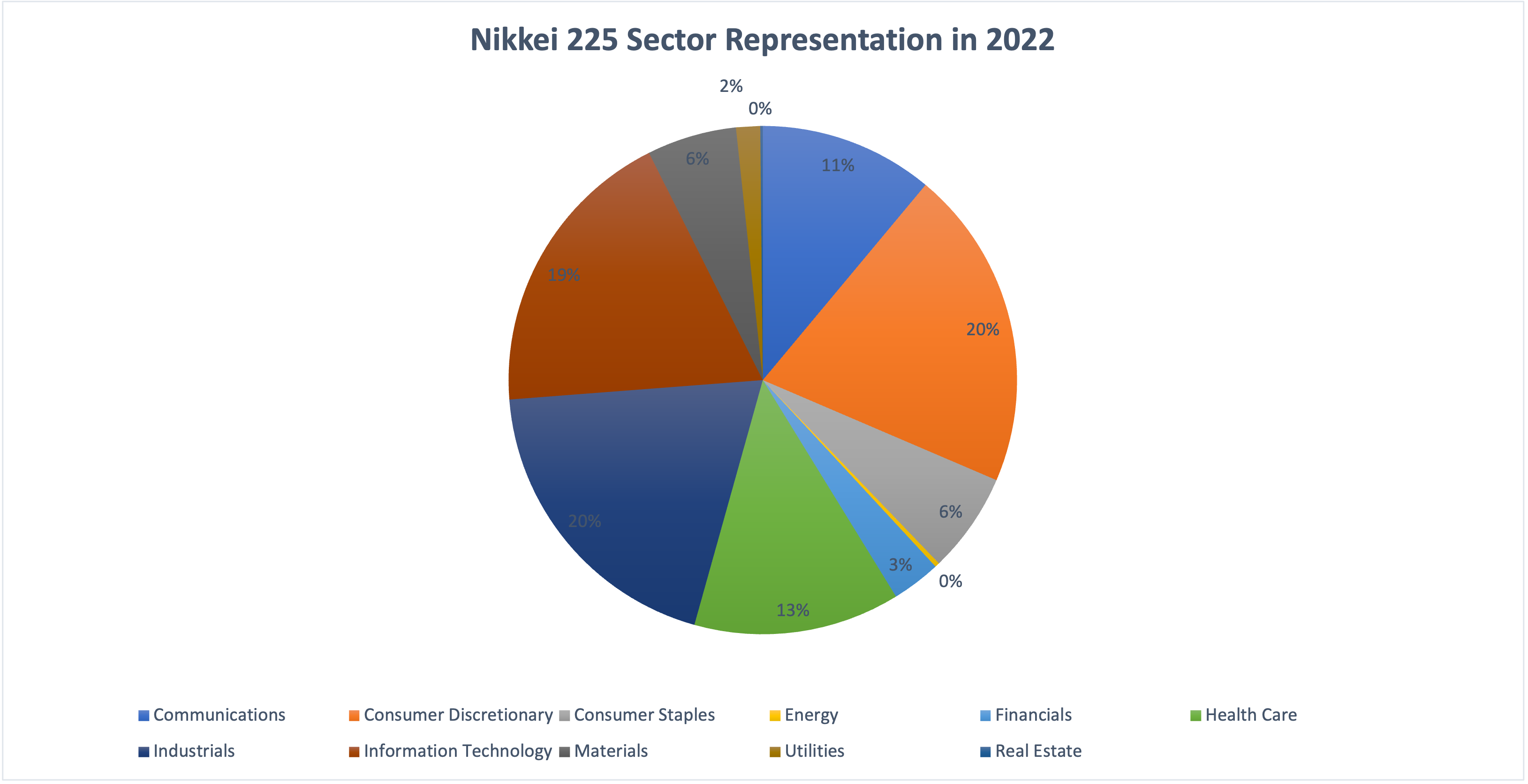
Table 2 below gives the sector representation of the Nikkei 225 index in terms of number of stocks and market capitalization as of January 31, 2023.

Table 2. Sector representation in the Nikkei 225 index.

Source: computation by the author (data: YahooFinance! financial website).

Calculation of the Nikkei 225 index value

The Nikkei 225 index is calculated using a price-weighted methodology. This means that the price of each stock in the index is multiplied by the number of shares outstanding to determine the total market value of the company. The Nikkei 225 index is frequently used as a leading indicator of the state of the Japanese stock market, and economy, and as a gauge of trends in the world economy.

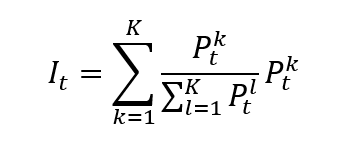
The formula to compute the Nikkei 225 is given by

A price-weighted index is calculated by summing the prices of all the assets in the index and dividing by a divisor equal to the number of assets.

The formula for a price-weighted index is given by

Price-weighted index value

where I is the index value, k a given asset, K the number of assets in the index, P^k the market price of asset k, and t the time of calculation of the index.

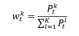
In a price-weighted index, the weight of asset k is given by formula can be rewritten as

Price-weighted index weight

which clearly shows that the weight of each asset in the index is its market price divided by the sum of the market prices of all assets.

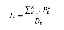
Note that the divisor, which is equal to the number of shares, is typically adjusted for events such as stock splits and dividends. The divisor is used to ensure that the value of the index remains consistent over time despite changes in the number of outstanding shares. A more general formula may then be:

Index value

Where D is the divisor which is adjusted over time to account for events such as stock splits and dividends.

Use of the Nikkei 225 index in asset management

Asset managers have shifted their attention in recent years to including environmental, social, and governance (ESG) factors in their investment choices. A number of ESG-related initiatives, such as the development of an ESG index that tracks businesses with high ESG scores, have been introduced by the Nikkei 225 index. The Nikkei 225 index may also be used by asset managers as a component of a more comprehensive global asset allocation strategy. For example, they may use the index to gain exposure to the Asian equity markets while also investing in other regions such as Europe and the Americas. In addition, the Nikkei 225 index can also be used as a risk management tool. Asset managers can spot potential risks and take action to reduce them by comparing a portfolio’s performance to the index.

Benchmark for equity funds

Equity funds that invest in Japanese stocks frequently use the Nikkei 225 index as a benchmark. The index is used by investment managers and individual investors to assess and contrast the performance of their holdings of Japanese equities with the performance of the overall market. Japanese exchange-traded funds (ETFs) and other investment products that follow the Japanese equity market use the index as a benchmark as well. Additionally, derivatives like futures and options that enable investors to trade on the Japanese equity market are based on the Nikkei 225 index.

Financial products around the Nikkei 225 index

There are several financial products that track the performance of the Nikkei 225 index, allowing investors to gain exposure to the Japanese stock market.

Nikkei 225 ETFs are a popular way for investors to gain exposure to the Japanese equity market, as they offer a low-cost and convenient way to invest in a diversified basket of stocks. Some of the largest Nikkei 225 ETFs by assets under management include the iShares Nikkei 225 ETF (NKY), the Nomura Nikkei 225 ETF (1321), and the Daiwa ETF Nikkei 225 (1320).
There are also mutual funds and index funds that track the Nikkei 225 index. These funds typically have higher fees than ETFs but may offer different investment strategies or options for investors.
Certificates are structured products that allow investors to gain exposure to the Nikkei 225 index without actually owning the underlying assets.
Futures contracts based on the Nikkei 225 index are also available for investors who want to trade the index with leverage or for hedging purposes. These futures contracts trade on the Osaka Exchange, a subsidiary of the Japan Exchange Group.

Historical data for the Nikkei 225 index

How to get the data?

The Nikkei 225 index is the most common index used in finance, and historical data for the Nikkei 225 index can be easily downloaded from the internet.

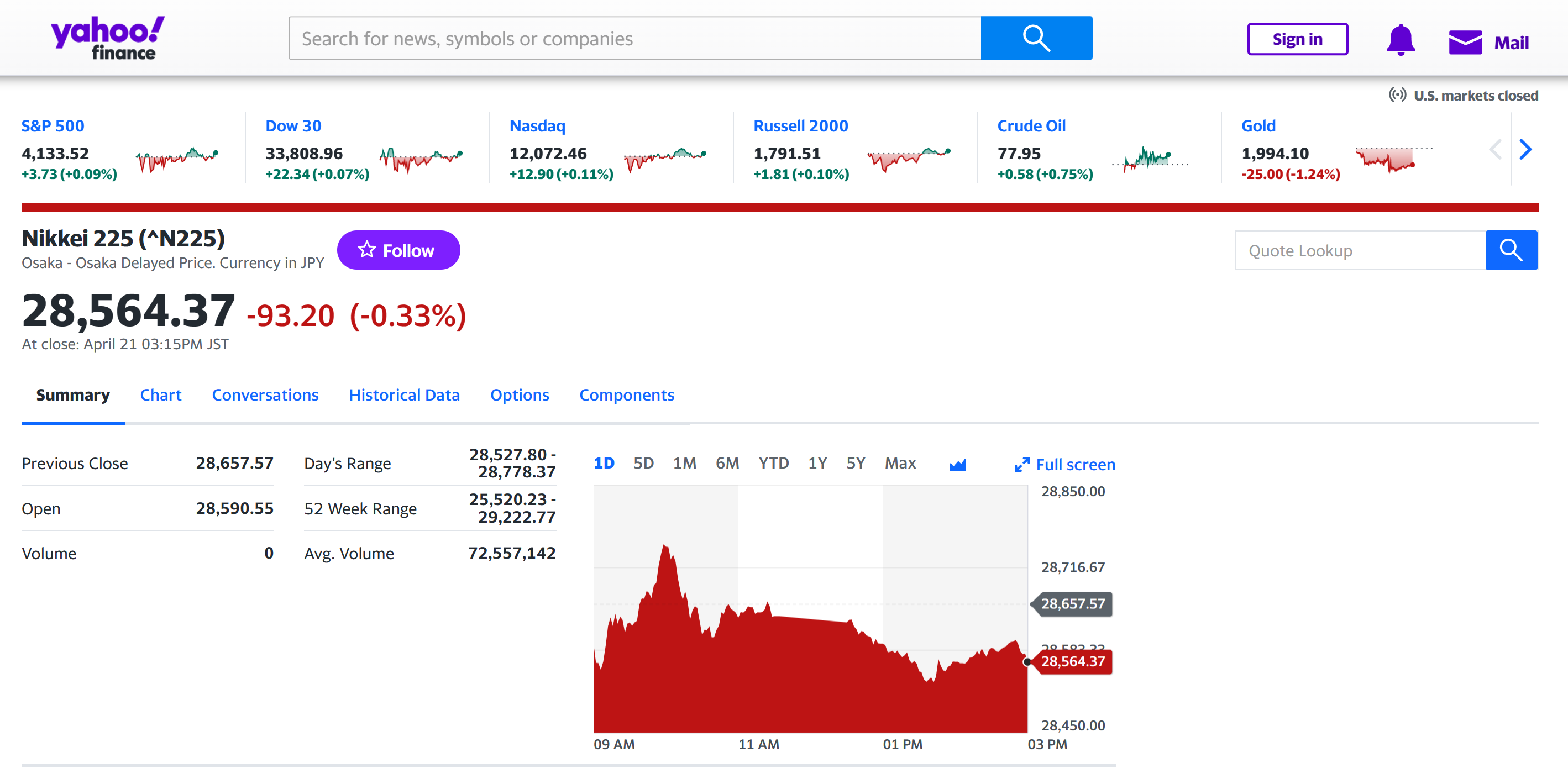
For example, you can download data for the Nikkei 225 index from March 1, 1990 on Yahoo! Finance (the Yahoo! code for Nikkei 225 index is ^N225).

Source: Yahoo! Finance.

You can also download the same data from a Bloomberg terminal.

R program

The R program below written by Shengyu ZHENG allows you to download the data from Yahoo! Finance website and to compute summary statistics and risk measures about the Nikkei 225 index.

Data file

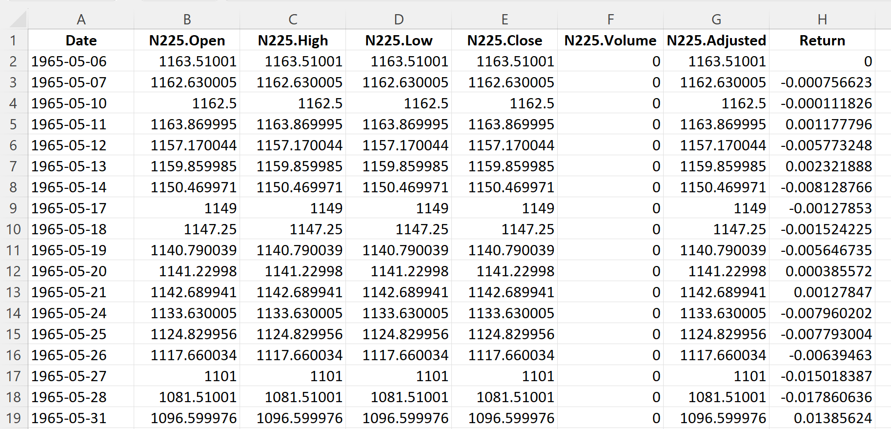
The R program that you can download above allows you to download the data for the Nikkei 225 index from the Yahoo! Finance website. The database starts on March 1, 1990. It also computes the returns (logarithmic returns) from closing prices.

Table 3 below represents the top of the data file for the Nikkei 225 index downloaded from the Yahoo! Finance website with the R program.

Table 3. Top of the data file for the Nikkei 225 index.
Top of the file for the Nikkei 225 index data
Source: computation by the author (data: Yahoo! Finance website).

Evolution of the Nikkei 225 index

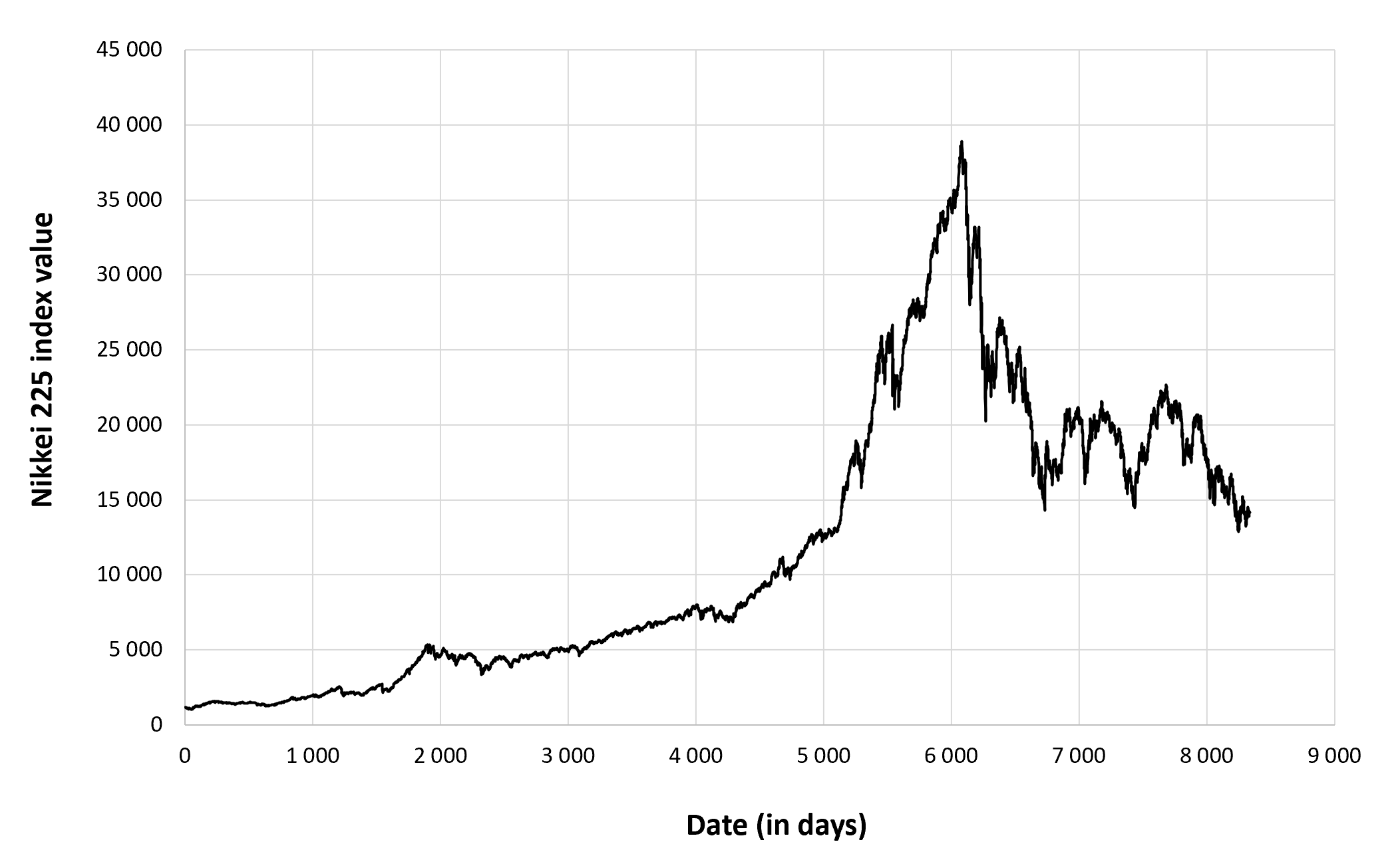
Figure 1 below gives the evolution of the Nikkei 225 index from March 1, 1990 to December 30, 2022 on a daily basis.

Figure 1. Evolution of the Nikkei 225 index.

Source: computation by the author (data: Yahoo! Finance website).

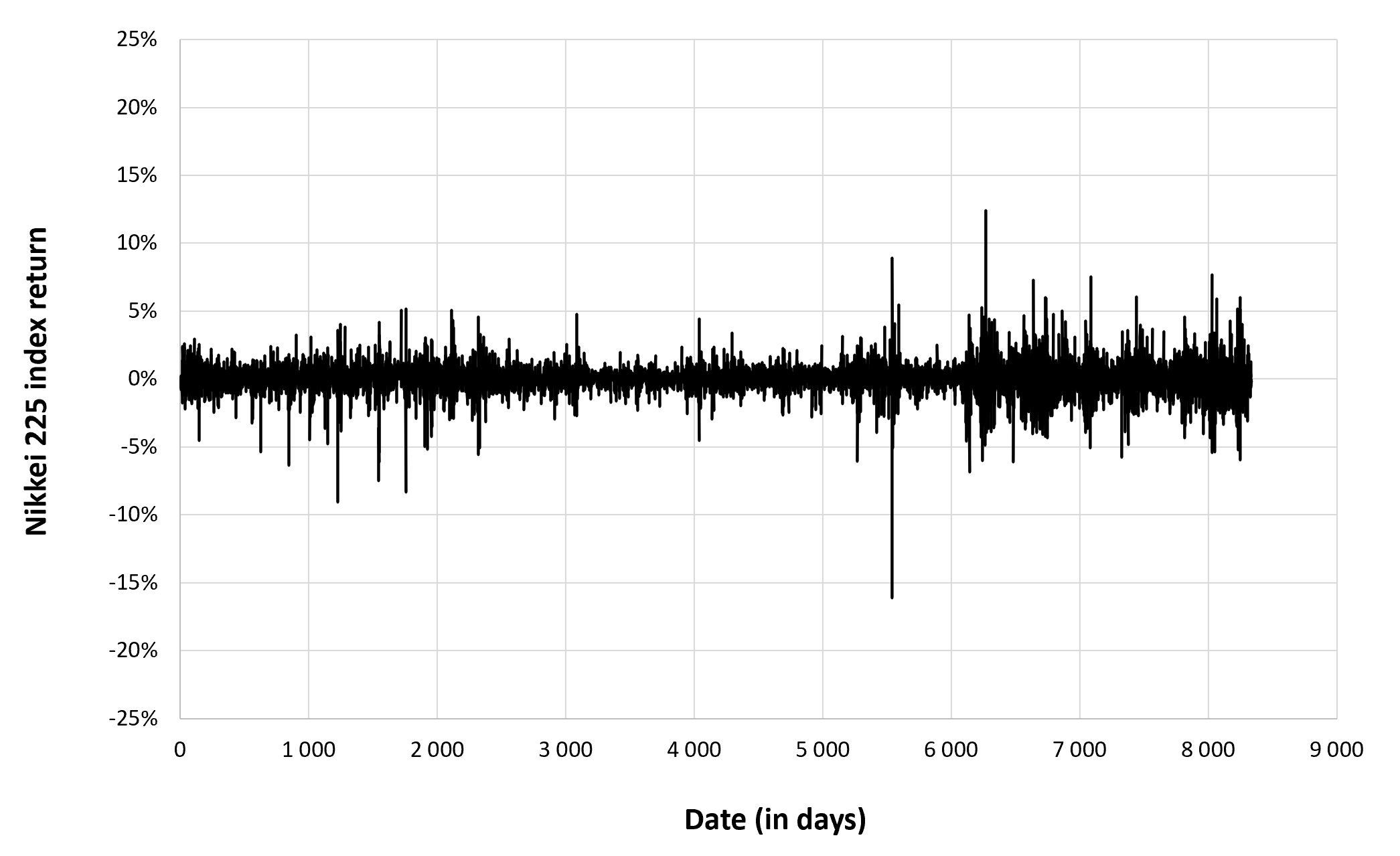
Figure 2 below gives the evolution of the Nikkei 225 index returns from March 1, 1990 to December 30, 2022 on a daily basis.

Figure 2. Evolution of the Nikkei 225 index returns.

Source: computation by the author (data: Yahoo! Finance website).

Summary statistics for the Nikkei 225 index

The R program that you can download above also allows you to compute summary statistics about the returns of the Nikkei 225 index.

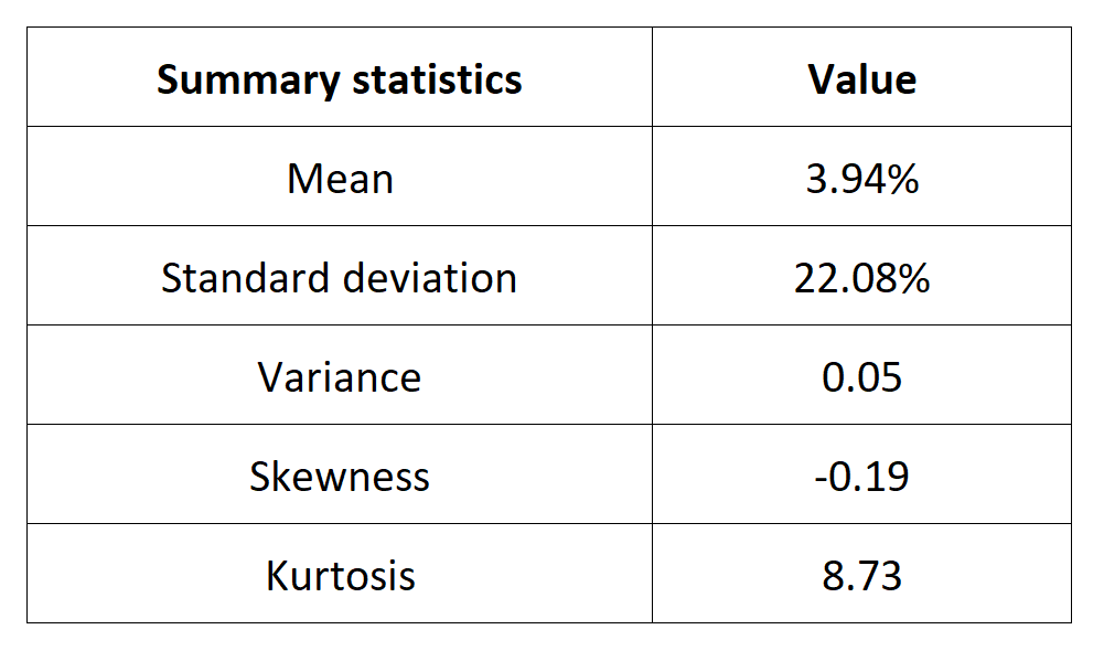
Table 4 below presents the following summary statistics estimated for the Nikkei 225 index:

The mean
The standard deviation (the squared root of the variance)
The skewness
The kurtosis.

The mean, the standard deviation / variance, the skewness, and the kurtosis refer to the first, second, third and fourth moments of statistical distribution of returns respectively.

Table 4. Summary statistics for the Nikkei 225 index.

Source: computation by the author (data: Yahoo! Finance website).

Statistical distribution of the Nikkei 225 index returns

Historical distribution

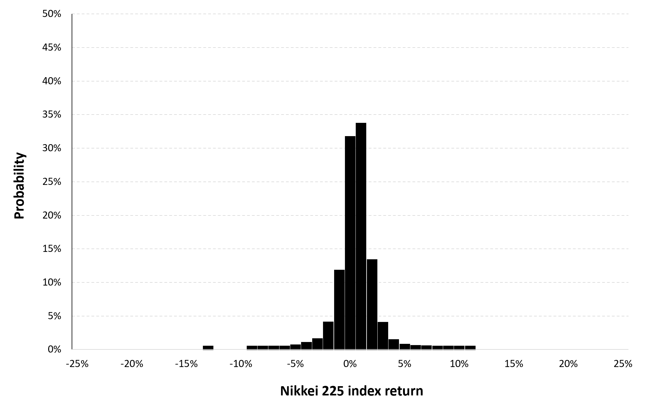
Figure 3 represents the historical distribution of the Nikkei 225 index daily returns for the period from March 1, 1990 to December 30, 2022.

Figure 3. Historical distribution of the Nikkei 225 index returns.

Source: computation by the author (data: Yahoo! Finance website).

Gaussian distribution

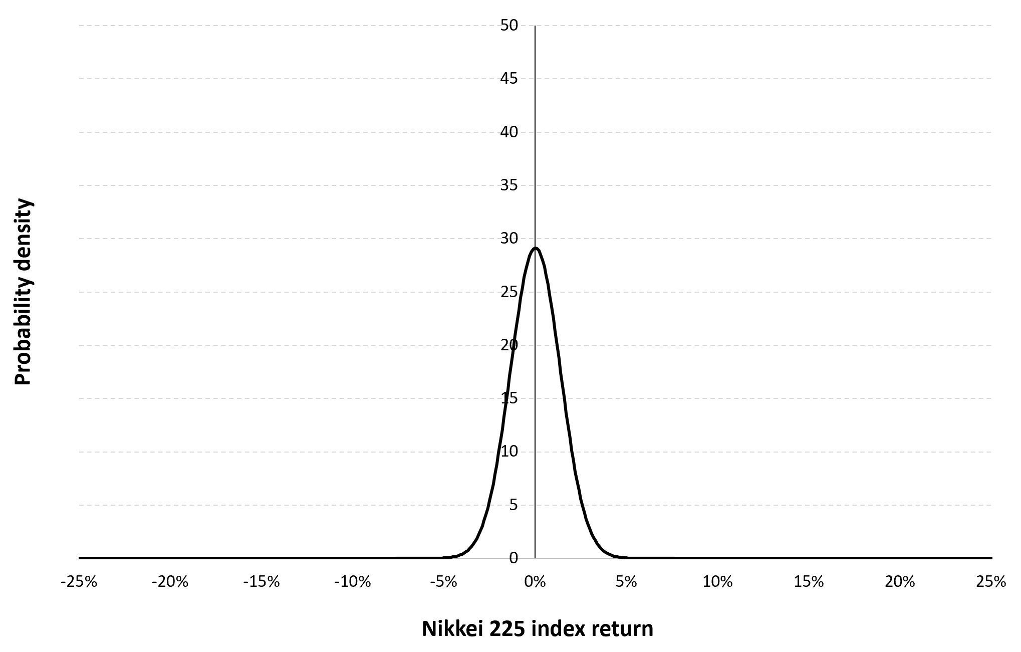
The Gaussian distribution (also called the normal distribution) is a parametric distribution with two parameters: the mean and the standard deviation of returns. We estimated these two parameters over the period from March 1, 1990 to December 30, 2022. The mean of daily returns is equal to 0.02% and the standard deviation of daily returns is equal to 1.37% (or equivalently 3.94% for the annual mean and 28.02% for the annual standard deviation as shown in Table 3 above).

Figure 4 below represents the Gaussian distribution of the Nikkei 225 index daily returns with parameters estimated over the period from March 1, 1990 to December 30, 2022.

Figure 4. Gaussian distribution of the Nikkei 225 index returns.
Gaussian distribution of the daily Nikkei 225 index returns
Source: computation by the author (data: Yahoo! Finance website).

Risk measures of the Nikkei 225 index returns

The R program that you can download above also allows you to compute risk measures about the returns of the Nikkei 225 index.

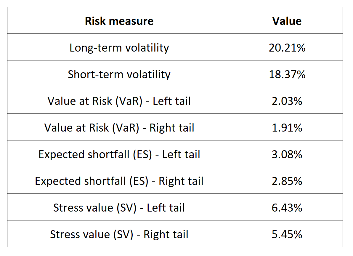
Table 5 below presents the following risk measures estimated for the Nikkei 225 index:

The long-term volatility (the unconditional standard deviation estimated over the entire period)
The short-term volatility (the standard deviation estimated over the last three months)
The Value at Risk (VaR) for the left tail (the 5% quantile of the historical distribution)
The Value at Risk (VaR) for the right tail (the 95% quantile of the historical distribution)
The Expected Shortfall (ES) for the left tail (the average loss over the 5% quantile of the historical distribution)
The Expected Shortfall (ES) for the right tail (the average loss over the 95% quantile of the historical distribution)
The Stress Value (SV) for the left tail (the 1% quantile of the tail distribution estimated with a Generalized Pareto distribution)
The Stress Value (SV) for the right tail (the 99% quantile of the tail distribution estimated with a Generalized Pareto distribution)

Table 5. Risk measures for the Nikkei 225 index.

Source: computation by the author (data: Yahoo! Finance website).

The volatility is a global measure of risk as it considers all the returns. The Value at Risk (VaR), Expected Shortfall (ES) and Stress Value (SV) are local measures of risk as they focus on the tails of the distribution. The study of the left tail is relevant for an investor holding a long position in the Nikkei 225 index while the study of the right tail is relevant for an investor holding a short position in the Nikkei 225 index.

Financial maps

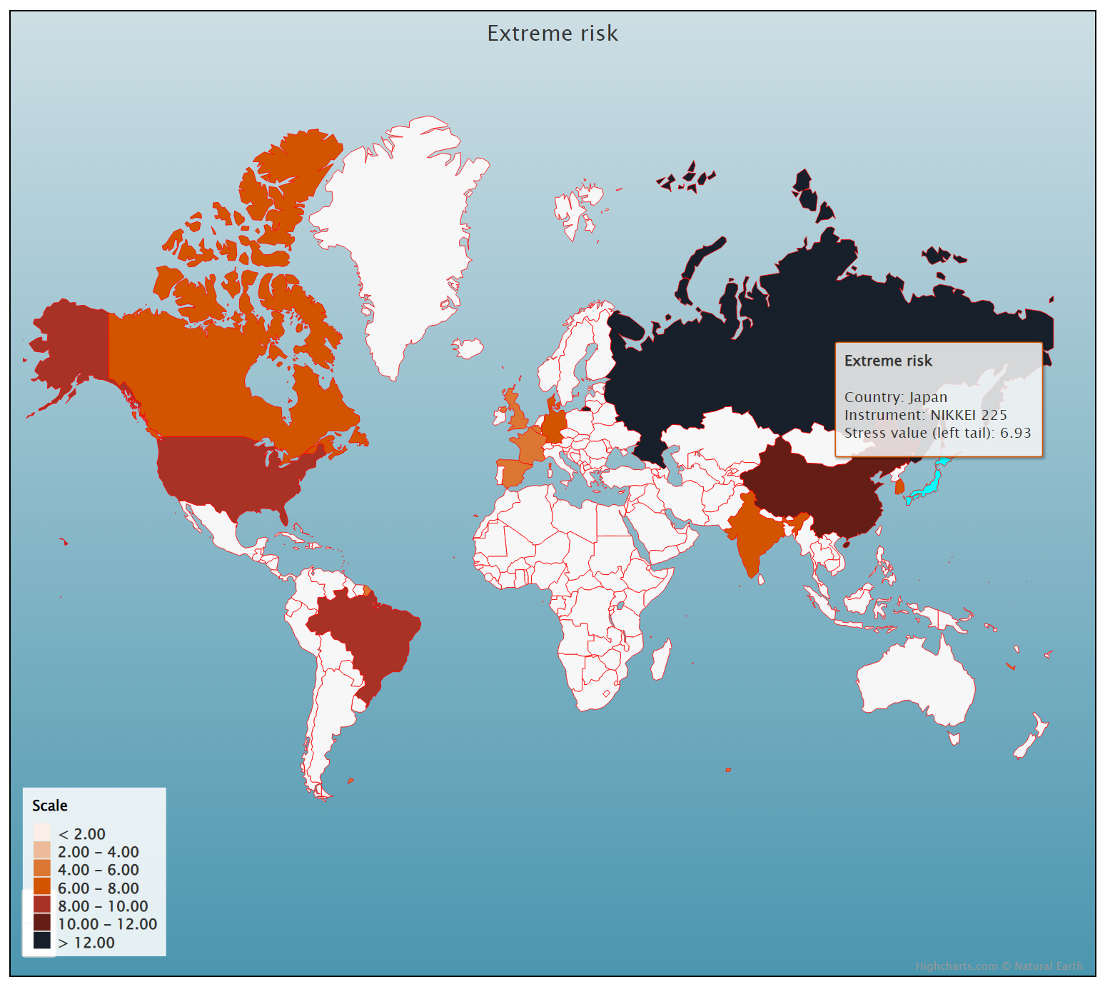
You can find financial world maps on the Extreme Events in Finance website. These maps represent the performance, risk and extreme risk in international equity markets.

Figure 5 below represents the world map for extreme risk estimated by the extreme value distribution (see Longin (2016 and 2000)).

Figure 5. Extreme risk map.

Source: Extreme Events in Finance.

Why should I be interested in this post?

For a number of reasons, management students (as future managers and individual investors) should learn about the Nikkei 225 index. The Nikkei 225 index is a key benchmark for the Japanese equity market, which is one of the world’s largest market. Understanding how the index is constructed, how it performs, and the companies that make up the index is important for anyone studying finance or business in Japan or interested in investing in Japanese equities.

Individual investors can assess the performance of their own investments in the Japanese equity market with the Nikkei 225 index. Last but not least, a lot of asset management firms base their mutual funds and exchange-traded funds (ETFs) on the Nikkei 225 index which can considered as interesting assets to diversify a portfolio. Learning about these products and their portfolio and risk management applications can be valuable for management students.

Useful resources

Academic research about risk

Longin F. (2000) From VaR to stress testing: the extreme value approach Journal of Banking and Finance, N°24, pp 1097-1130.

Longin F. (2016) Extreme events in finance: a handbook of extreme value theory and its applications Wiley Editions.

Data

Yahoo! Finance

Yahoo! Finance Nikkei 225 index

Other

Extreme Events in Finance

Extreme Events in Finance Risk maps

Wikipedia Nikkei 225

About the author

The article was written in April 2023 by Nithisha CHALLA (ESSEC Business School, Grande Ecole Program – Master in Management, 2021-2023).

Implied Volatility

May 15, 2022 by Jayati WALIA

In this article, Jayati WALIA (ESSEC Business School, Grande Ecole Program – Master in Management, 2019-2022) explains how implied volatility is computed from option market prices and a option pricing model.

Introduction

Volatility is a measure of fluctuations observed in an asset’s returns over a period of time. The standard deviation of historical asset returns is one of the measures of volatility. In option pricing models like the Black-Scholes-Merton model, volatility corresponds to the volatility of the underlying asset’s return. It is a key component of the model because it is not directly observed in the market and cannot be directly computed. Moreover, volatility has a strong impact on the option value.

Mathematically, in a reverse way, implied volatility is the volatility of the underlying asset which gives the theoretical value of an option (as computed by Black-Scholes-Merton model) equal to the market price of that option.

Implied volatility is a forward-looking measure because it is a representation of expected price movements in an underlying asset in the future.

Computation methods for implied volatility

The Black-Scholes-Merton (BSM) model provides an analytical formula for the price of both a call option and a put option.

The value for a call option at time t is given by:

Call option value

The value for a put option at time t is given by:

Put option value

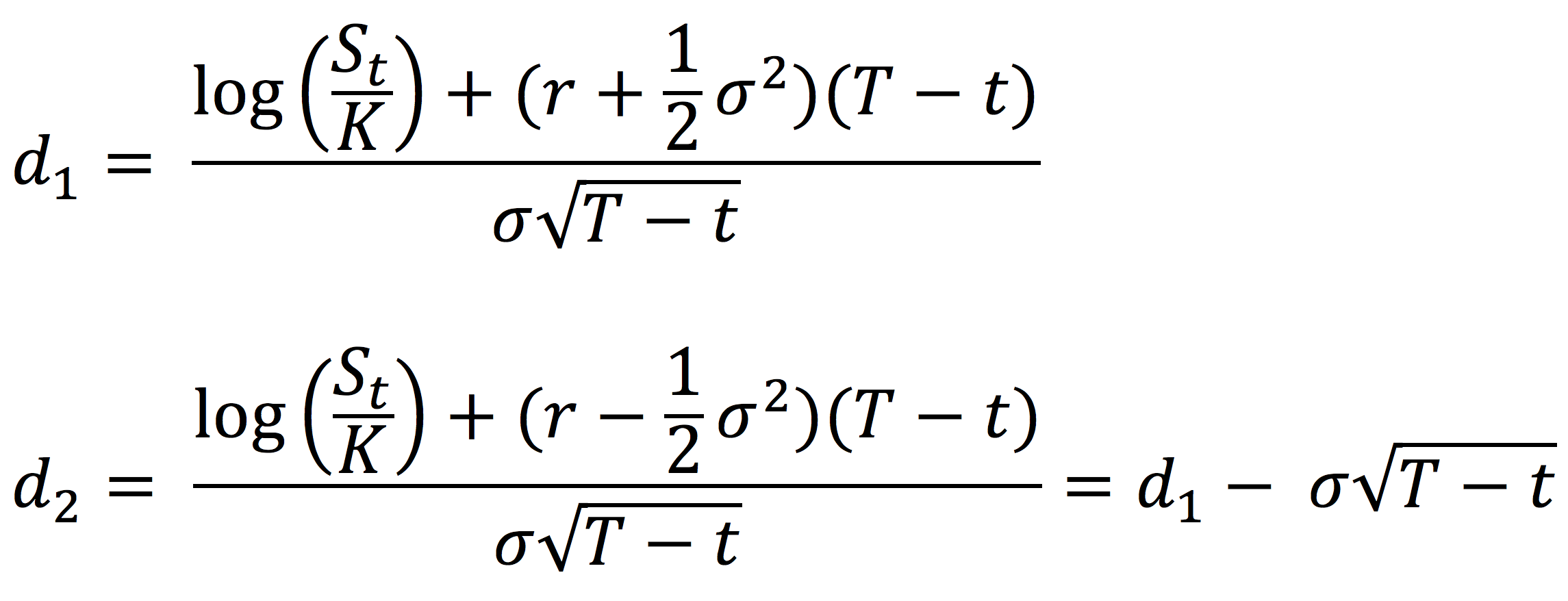
where the parameters d₁ and d₂ are given by:,

call option d1 d2

with the following notations:

S_t : Price of the underlying asset at time t
t: Current date
T: Expiry date of the option
K: Strike price of the option
r: Risk-free interest rate
σ: Volatility of the underlying asset
N(.): Cumulative distribution function for a normal (Gaussian) distribution. It is the probability that a random variable is less or equal to its input (i.e. d₁ and d₂) for a normal distribution. Thus, 0 ≤ N(.) ≤ 1

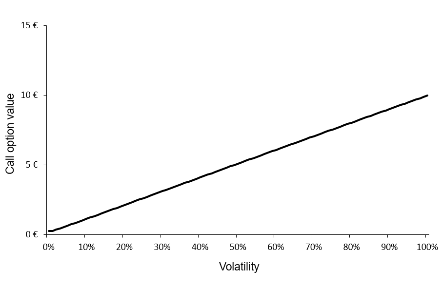
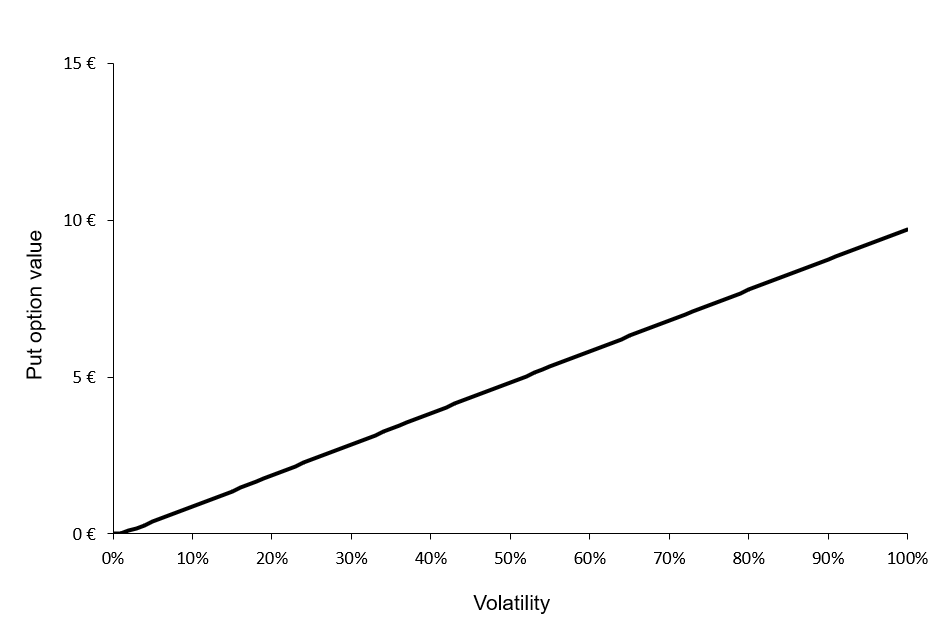
From the BSM model, both for a call option and a put option, the option price is an increasing function of the volatility of the underlying asset: an increase in volatility will cause an increase in the option price.

Figures 1 and 2 below illustrate the relationship between the value of a call option and a put option and the level of volatility of the underlying asset according to the BSM model.

Figure 1. Call option value as a function of volatility.

Source: computation by the author (BSM model)

Figure 2. Put option value as a function of volatility.

Source: computation by the author (BSM model)

You can download below the Excel file for the computation of the value of a call option and a put option for different levels of volatility of the underlying asset according to the BSM model.

We can observe that the call and put option values are a monotonically increasing function of the volatility of the underlying asset. Then, for a given level of volatility, there is a unique value for the call option and a unique value for the put option. This implies that this function can be reversed; for a given value for the call option, there is a unique level of volatility, and similarly, for a given value for the put option, there is a unique level of volatility.

The BSM formula can be reverse-engineered to compute the implied volatility i.e., if we have the market price of the option, the market price of the underlying asset, the market risk-free rate, and the characteristics of the option (the expiration date and strike price), we can obtain the implied volatility of the underlying asset by inverting the BSM formula.

Example

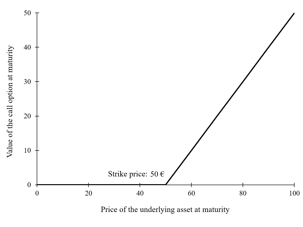
Consider a call option with a strike price of 50 € and a time to maturity of 0.25 years. The market risk-free interest rate is 2% and the current price of the underlying asset is 50 €. Thus, the call option is ‘at-the-money’. If the market price of the call option is equal to 2 €, then the associated level of volatility (implied volatility) is equal to 18.83%.

You can download below the Excel file below to compute the implied volatility given the market price of a call option. The computation uses the Excel solver.

Volatility smile

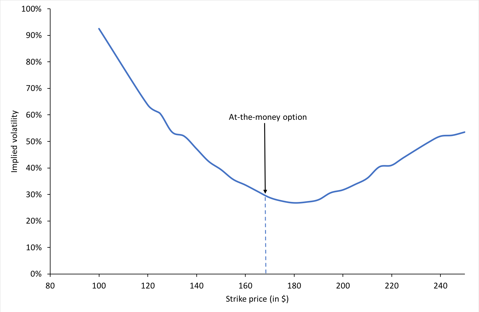
Volatility smile is the name given to the plot of implied volatility against different strikes for options with the same time to maturity. According to the BSM model, it is a horizontal straight line as the model assumes that the volatility is constant (it does not depend on the option strike). However, in practice, we do not observe a horizontal straight line. The curve may be in the shape of the alphabet ‘U’ or a ‘smile’ which is the usual term used to refer to the observed function of implied volatility.

Figure 3 below depicts the volatility smile for call options on the Apple stock on May 13, 2022.

Figure 3. Volatility smile for call options on Apple stock.
Apple volatility smile
Source: Computation by author.

We can also observe that the for a specific time to maturity, the implied volatility is minimum when the option is at-the-money.

Volatility surface

An essential assumption of the BSM model is that the returns of the underlying asset follow geometric Brownian motion (corresponding to log-normal distribution for the price at a given point in time) and the volatility of the underlying asset price remains constant over time until the expiration date. Thus theoretically, for a constant time to maturity, the plot of implied volatility and strike price would be a horizontal straight line corresponding to a constant value for volatility.

Volatility surface is obtained when values for implied volatilities are calculated for options with different strike prices and times to maturity.

CBOE Volatility Index

The Chicago Board Options Exchange publishes the renowned Volatility Index (also known as VIX) which is an index based on the implied volatility of 30-day option contracts on the S&P 500 index. It is also called the ‘fear gauge’ and it is a representation of the market outlook for volatility for the next 30 days.

Useful resources

Academic articles

Black F. and M. Scholes (1973) “The Pricing of Options and Corporate Liabilities” The Journal of Political Economy, 81, 637-654.

Dupire B. (1994). “Pricing with a Smile” Risk Magazine 7, 18-20.

Merton R.C. (1973) “Theory of Rational Option Pricing” Bell Journal of Economics, 4, 141–183.

Business

CBOE Volatility Index (VIX)

CBOE VIX tradable products

About the author

The article was written in May 2022 by Jayati WALIA (ESSEC Business School, Grande Ecole Program – Master in Management, 2019-2022).

Risk Aversion

April 14, 2022 by Diana Carolina SARMIENTO PACHON

Risk Aversion

In this article, Diana Carolina SARMIENTO PACHON (ESSEC Business School, Master in Strategy & Management of International Business (SMIB), 2021-2022) explains the economic concept of risk aversion, which is key to understand the behavior of participants in financial markets.

Risk Aversion refers to the level of reluctance that an individual possesses towards risk. Specifically, it refers to the attitude of investors towards the risk underlying investments which will directly determine how portfolios are allocated or even how a stock may behave depending on market conditions. To elaborate, when market participants have higher risk aversion due to unfavorable market shocks e.g., natural disasters, bad news or scandals that affect a company or a security, this situation will cause a perception of higher risk leading to many selling, and thus decreasing prices. Therefore, risk aversion should be analyzed carefully.

Risk aversion and investor’s characteristics

It’s important to note that risk aversion can be highly variable over time as this notion changes along with investor profile, in other words with age, income, culture and other key factors, making it even more complex to evaluate than it appears in the traditional economics literature. To illustrate more accurately some of the factors that define an investor profile are:

Age

The older the person is, the more risk averse he or she is. On the contrary, younger individuals tend to be less risk averse which may be due to their high expectations and eagerness to attempt something new as well as the longer timeframe they have, whereas older people prefer safety and stability in their lives.

Income

Individuals with a smaller budget tend to have a higher risk aversion since they have fewer resources, and a loss would make a greater impact on them than a wealthy individual.

Past Losses

When an individual has already experienced some loss, she or he will be more wary of it since it’s now too costly to bear another loss; therefore, risk aversion will be significantly higher. An example of this is the post-crisis, as people have lost so much and this has had a negative impact on their lives, they tend to become more cautious of risk.

Investment Objective

For crucial events such as retirement or education, risk version tends to be higher as the individual cannot bear to risk for such a fundamental matter of his or her life.

Investment Horizon

Investors focused on short-term horizon tend to be more risk averse as they cannot take too much risk due to the short timeline.

Risk aversion and financial investments

Furthermore, risk aversion also takes into account more factors apart from those mentioned above, for this reason most of the time before creating the respective portfolio for an investor, financial advisors shape their client’s risk preferences in order to adjust the portfolio allocation to them. Many times, these can be conducted by questionnaires and tests that will accordingly assign a risk profile concluding with certain risk categories:

A Conservative profile refers to more risk averse individuals, the portfolios assigned for this type are mainly composed by both more secure & less volatile securities such as bonds, meanwhile stocks have a minimal participation.
A Moderate profile is attributed to more risk averse individuals who are willing to take more risk, however he or she does not want to step too much further. These portfolios are usually more diversified as they contain more types of securities in different percentages such as government & corporate bonds, and stocks.
An aggressive profile which is allocated to portfolios mainly composed in the highest percentage by the risky securities. For instance, the main securities could be stocks, specifically growth stocks or even crypto.

Due to all sensitive and private information used by financial institutions, financial regulatory entities are important to ensure the protection and transparency of information, thereby the Mifid (The Markets in Financial Instruments Directive) has been created in the European Union to fulfill such task through the use of rules and general standards.

Measure of risk of financial assets

Additionally, there are other mathematical metrics that can interfere in the risk profile, and depending on these the portfolio may be constructed:

Standard Deviation

It refers to the volatility of historical data, in other words how dispersed the data is over time which illustrates how risky the security may be. The higher the standard deviation, the higher the risk since this is suggesting that the stock is more variable and there is more uncertainty, thus a risk averse individual prefers a lower standard deviation.

Beta

It is linked with the systematic risk that comes with a stock, that is to say it illustrates the volatility compared to the market. Firstly, a beta equal to 1 indicates a volatility and movement equalizing the market, secondly a beta higher than 1 is referred to a security that is more volatile than the market, to illustrate B= 1.50 specifies 50% more volatility than the market. Thirdly, a beta less than 1 stipulates less volatility than the market. Therefore, the lower the beta the less risk exposure is found.

Modern Portfolio Theory & Risk

Introduced by Harry Markowitz in 1950s, the Modern Portfolio Theory illustrates the optimum portfolio allocation that maximizes return given a specific level of risk, in which risk is measured by the standard deviation and the return by the average mean of the portfolio. This explanation also leads to the one- single period mean-variance theory which suggests various portfolio allocations depending on the trade-off between return and risk. However, there are more advance models which explain this scenario in a multiperiod by rebalancing or diversifying further.

Risk aversion and economic conditions

Risk aversion does not only shape the portfolio allocation and its diversification, but it also may have a significant impact on the market as a result of expectations. When there are booming economic times, individuals usually feel more confident and thus less risk averse as a consequence of positive expectations of future cash flows; however, when a recession is coming investors may shift to a more risk averse behavior making them feel afraid of the future which influences them to sell certain stocks and, in this way, making the price plump. Although it may be seen as a simple emotion that defines the fear of risk, it still impacts in a very large extent the financial market as it dictates the roles and strategies behind investing, and thereby it is crucial analyze it carefully.

▶ Youssef LOURAOUI Markowitz Modern Portfolio Theory

▶ Youssef LOURAOUI Implementing Markowitz asset allocation model

▶ Jayati WALIA Capital Asset Pricing Model (CAPM)

Useful resources

Díaz A and Esparcia C (2019) Assessing Risk Aversion From the Investor’s Point of View Frontiers in Psychology, 10:1490

Desjardins Online brokerage The Risk Aversion Coefficient

Coursera course Investment management

Crehana course Trading: How to invest in stocks (Trading: Como invertir en Bolsa)

About the author

The article was written in April 2022 by Diana Carolina SARMIENTO PACHON (ESSEC Business School, Master in Strategy & Management of International Business (SMIB), 2021-2022)

The incredible story of Nick Leeson & the Barings Bank

March 17, 2022 by Louis DETALLE

The incredible story of Nick Leeson & the Barings Bank

In this article, Louis DETALLE (ESSEC Business School, Grande Ecole Program – Master in Management, 2020-2023) looks back at the bank fraud of Nick Leeson, a trader at Barings, which led to the collapse of the UK’s oldest investment bank…

History of Barings and Nick Leeson’s background

Barings was founded in 1762 in the UK, making it the oldest British bank, so renowned and prestigious that even the Queen of England was a client. It is therefore in this renowned institution that Nick Leeson will pursue his career after a spell at Morgan Stanley as an operations assistant. Ambitious and ready to do anything to make a name for himself within this prestigious institution, Nick Leeson multiplies risky operations and gradually climbs the ladder, greeted by a management admiring his results considering his young age.

The great fraud

In 1990, Barings chose Nick Leeson to head up the management of its Singapore subsidiary. Having spotted a flaw in the system for monitoring the compliance of traders’ market operations, Nick Leeson carried out speculative operations that were normally unauthorised and that brought in a lot of money for Barings. Nick Leeson was therefore engaged in a series of successful speculative trades, which is why management did not look into the matter. However, the day comes when the trader’s luck runs out: he makes bigger and bigger losses, as he hopes to make up for previous losses with each new trade.

With the trade tracking loophole still in use by Nick Leeson, he hides the losses from the failed trades in an error account, 88888. Nick Leeson also concealed documents from the bank’s auditor and continued to trade with losses accumulating over time. By the beginning of 1995, these losses reached £210 million, which represented half of Barings’ capital.

Eager to wipe out these very large losses, on the evening of January 16, 1995 Nick made a colossal trade – $7 billion – betting that the Nikkei would not fall overnight. Normally this would be considered a low-risk trade, but on the evening of 16 January an earthquake struck Kobe. On the morning of January 17, the Nikkei price collapsed and so did the trader’s positions.

Nick Leeson tried to make up for it by trying to make a quick recovery in the Nikkei, but this did not happen. Nick’s losses reach an abysmal $1.4 billion, which is twice the bank’s capital. Despite Nick’s ability to circumvent the bank’s internal controls, the level of losses is such that his entire scheme is uncovered. And the bank, faced with such losses, is forced to declare bankruptcy.

Conclusion

In conclusion, it was a major error in the compliance system that caused the Barings bankruptcy. Nowadays, enforcers can no longer supervise the tasks entrusted to them, and this is all the more true in banks where brand new departments have been created since the 2000s with the rise of compliance and banking regulation.

Useful resources

Mousli M. (2015) Quand un trader fait sauter une banque : Nick Leeson et la Barings L’Économie politique 68(4) 89-101.

Comprehensive history of the Barings bank

About the author

The article was written in March 2022 by Louis DETALLE (ESSEC Business School, Grande Ecole Program – Master in Management, 2020-2023).

What happened between Bruno Iksil & JP Morgan

February 5, 2024March 17, 2022 by Louis DETALLE

What happened between Bruno Iksil & JP Morgan

In this article, Louis DETALLE (ESSEC Business School, Grande Ecole Program – Master in Management, 2020-2023) explains how Bruno Iksil, a French trader working in London made inconsiderate trades in the name of the renown JP Morgan.

Bruno Iksil: background of a French trader based in London

Bruno Iksil, known as “The Whale”, is a French trader well known in London financial circles. A former student of Centrale Paris, this former Natixis employee built a reputation at JP Morgan for the size of the orders he placed. Bruno Iksil worked on the Credit Default Swaps (CDS) market, financial products that provide insurance against the non-repayment of loans.

Iksil’s activities at JP Morgan

Bruno Iksil’s reckless trading initially made JP Morgan Chase a lot of money, almost $100 million. His ability to succeed brilliantly in times of crisis and his boldness in business were praised and rewarded on numerous occasions by management, which made Iksil the highest paid trader in London. According to the Wall Street Journal, in recent years Bruno Iksil earned around $100 million a year at JPMorgan’s chief investment office (CIO).

And his nickname, linked to the enormity of the commitments he was making, was regularly on the front page of all the newspapers, along with the new positions taken by ‘The Whale’.

JP Morgan’s losses

Bruno Iksil was suspected of being involved in a colossal loss by JP Morgan Chase. According to the latest estimates, the risky bets of the Frenchman and his colleagues cost JP Morgan Chase 5.8 billion dollars. This triggered a real storm in the life of the trader who, according to the British journalist The Guardian, left the company.

Following the losses incurred by the American bank, Jamie Dimon – the Chief Executive Officer – had announced losses amounting to 2 billion dollars. In fact, nearly 4.4 billion dollars were lost as a result of the Whale’s operations.

Following these announcements, the bank’s market capitalization plunged by 25 billion dollars as the stock dived by 9%.

Conclusion and aftermath of the affair

The whale affair brought to light accusations of negligence against the bank, particularly in its internal controls. The risky positions in credit derivatives that Bruno Iksil and many other banks regularly took contributed to the subprime crisis. As a result, JP Morgan was fined $1 billion by the British and American authorities, on behalf of its management that enable the Whale to invest so much on financial markets.

Useful resources

Philippe Bernard (13/07/2015) A Londres, Bruno Michel Iksil échappe aux poursuites Le Monde.

JP Morgan

About the author

The article was written in March 2022 by Louis DETALLE (ESSEC Business School, Grande Ecole Program – Master in Management, 2020-2023).

The historical method for VaR calculation

January 30, 2024December 17, 2021 by Jayati WALIA

In this article, Jayati WALIA (ESSEC Business School, Grande Ecole Program – Master in Management, 2019-2022) presents the historical method for VaR calculation.

Introduction

A key factor that forms the backbone for risk management is the measure of those potential losses that an institution is exposed to any investment. Various risk measures are used for this purpose and Value at Risk (VaR) is the most commonly used risk measure to quantify the level of risk and implement risk management.

VaR is typically defined as the maximum loss which should not be exceeded during a specific time period with a given probability level (or ‘confidence level’). VaR is used extensively to determine the level of risk exposure of an investment, portfolio or firm and calculate the extent of potential losses. Thus, VaR attempts to measure the risk of unexpected changes in prices (or return rates) within a given period. Mathematically, the VaR corresponds to the quantile of the distribution of returns.

The two key elements of VaR are a fixed period of time (say one or ten days) over which risk is assessed and a confidence level which is essentially the probability of the occurrence of loss-causing event (say 95% or 99%). There are various methods used to compute the VaR. In this post, we discuss in detail the historical method which is a popular way of estimating VaR.

Calculating VaR using the historical method

Historical VaR is a non-parametric method of VaR calculation. This methodology is based on the approach that the pattern of historical returns is indicative of the pattern of future returns.

The first step is to collect data on movements in market variables (such as equity prices, interest rates, commodity prices, etc.) over a long time period. Consider the daily price movements for CAC40 index within the past 2 years (512 trading days). We thus have 512 scenarios or cases that will act as our guide for future performance of the index i.e., the past 512 days will be representative of what will happen tomorrow.

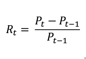
For each day, we calculate the percentage change in price for the CAC40 index that defines our probability distribution for daily gains or losses. We can express the daily rate of returns for the index as:
img_historicalVaR_returns_formula

Where R_t represents the (arithmetic) return over the period [t-1, t] and P_t the price at time t (the closing price for daily data). Note that the logarithmic return is sometimes used (see my post on Returns).

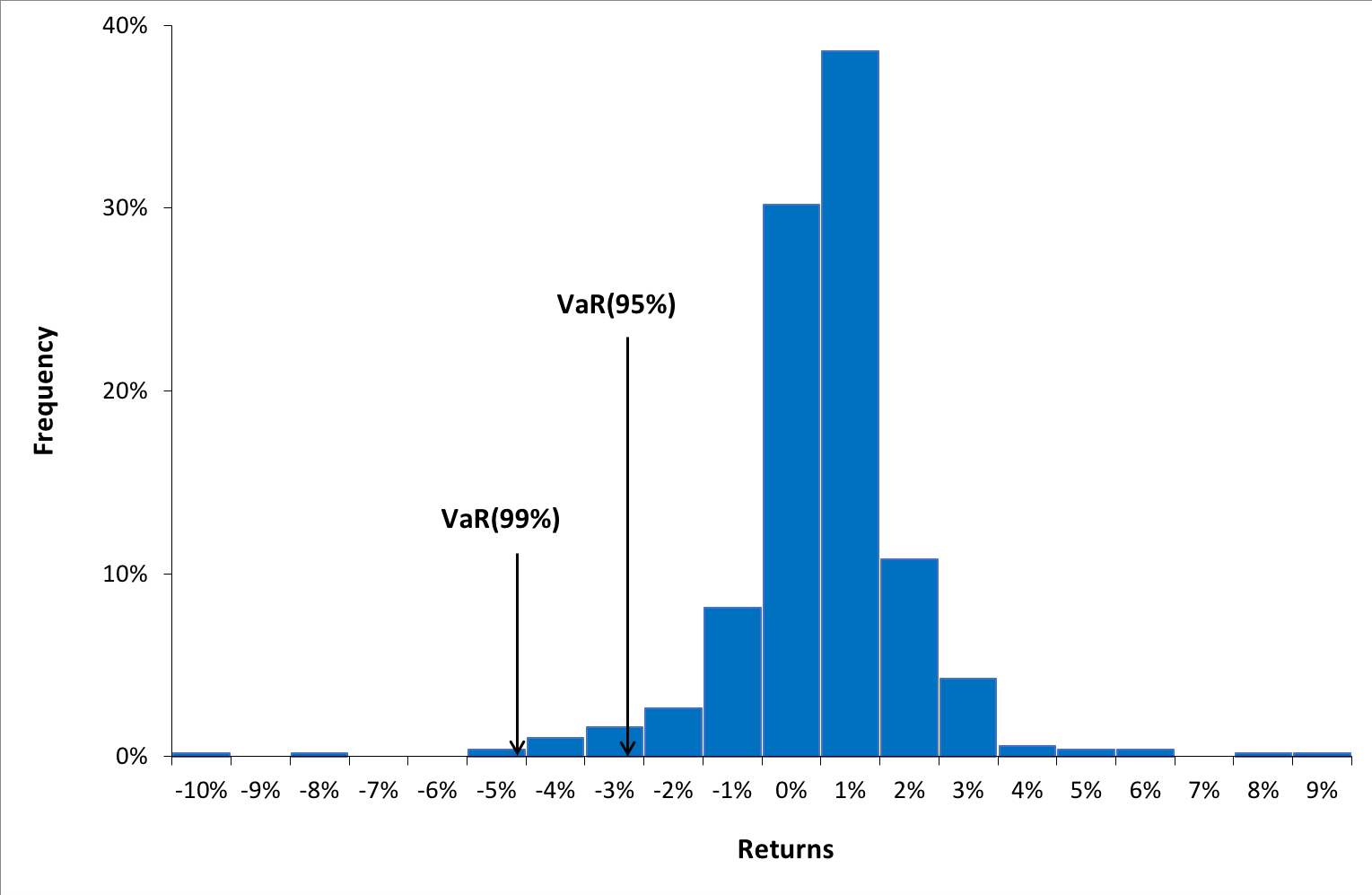
Next, we sort the distribution of historical returns in ascending order (basically in order of worst to best returns observed over the period). We can now interpret the VaR for the CAC40 index in one-day time horizon based on a selected confidence level (probability).

Since the historical VaR is estimated directly from data without estimating or assuming any other parameters, hence it is a non-parametric method.

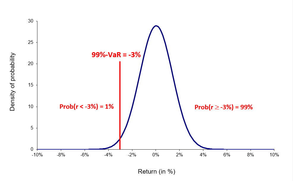
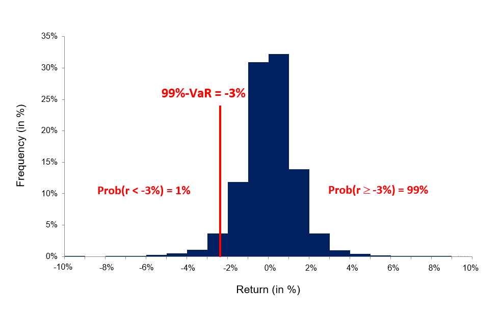
For instance, if we select a confidence level of 99%, then our VaR estimate corresponds to the 1st percentile of the probability distribution of daily returns (the top 1% of worst returns). In other words, there are 99% chances that we will not obtain a loss greater than our VaR estimate (for the 99% confidence level). Similarly, VaR for a 95% confidence level corresponds to top 5% of the worst returns.

Figure 1. Probability distribution of returns for the CAC40 index.
Historical method VaR
Source: computation by the author (data source: Bloomberg).

You can download below the Excel file for the VaR calculation with the historical method. The historical distribution is estimated with historical data from the CAC 40 index.

From the above graph, we can interpret VaR for 90% confidence level as -3.99% i.e., there is a 90% probability that daily returns we obtain in future are greater than -3.99%. Similarly, VaR for 99% confidence level as -5.60% i.e., there is a 99% probability that daily returns we obtain in future are greater than -5.60%.

Advantages and limitations of the historical method

The historical method is a simple and fast method to calculate VaR. For a portfolio, it eliminates the need to estimate the variance-covariance matrix and simplifies the computations especially in cases of portfolios with a large number of assets. This method is also intuitive. VaR corresponds to a large loss sustained over an historical period that is known. Hence users can go back in time and explain the circumstances behind the VaR measure.

On the other hand, the historical method has a few of drawbacks. The assumption is that the past represents the immediate future is highly unlikely in the real world. Also, if the horizon window omits important events (like stock market booms and crashes), the distribution will not be well represented. Its calculation is only as strong as the number of correct data points measured that fully represent changing market dynamics even capturing crisis events that may have occurred such as the Covid-19 crisis in 2020 or the financial crisis in 2008. In fact, even if the data does capture all possible historical dynamics, it may not be sufficient because market will never entirely replicate past movements. Finally, the method assumes that the distribution is stationary. In practice, there may be significant and predictable time variation in risk.

Useful resources

Jorion, P. (2007) Value at Risk , Third Edition, Chapter 10 – VaR Methods, 276-279.

Longin F. (2000) From VaR to stress testing : the extreme value approach Journal of Banking and Finance, 24, 1097-1130.

About the author

The article was written in December 2021 by Jayati WALIA (ESSEC Business School, Grande Ecole Program – Master in Management, 2019-2022).

The variance-covariance method for VaR calculation

January 30, 2024December 17, 2021 by Jayati WALIA

In this article, Jayati WALIA (ESSEC Business School, Grande Ecole – Master in Management, 2019-2022) presents the variance-covariance method for VaR calculation.

Introduction

The two key elements of VaR are a fixed period of time (say one or ten days) over which risk is assessed and a confidence level which is essentially the probability of the occurrence of loss-causing event (say 95% or 99%). There are various methods used to compute the VaR. In this post, we discuss in detail the variance-covariance method for computing value at risk which is a parametric method of VaR calculation.

Assumptions

The variance-covariance method uses the variances and covariances of assets for VaR calculation and is hence a parametric method as it depends on the parameters of the probability distribution of price changes or returns.

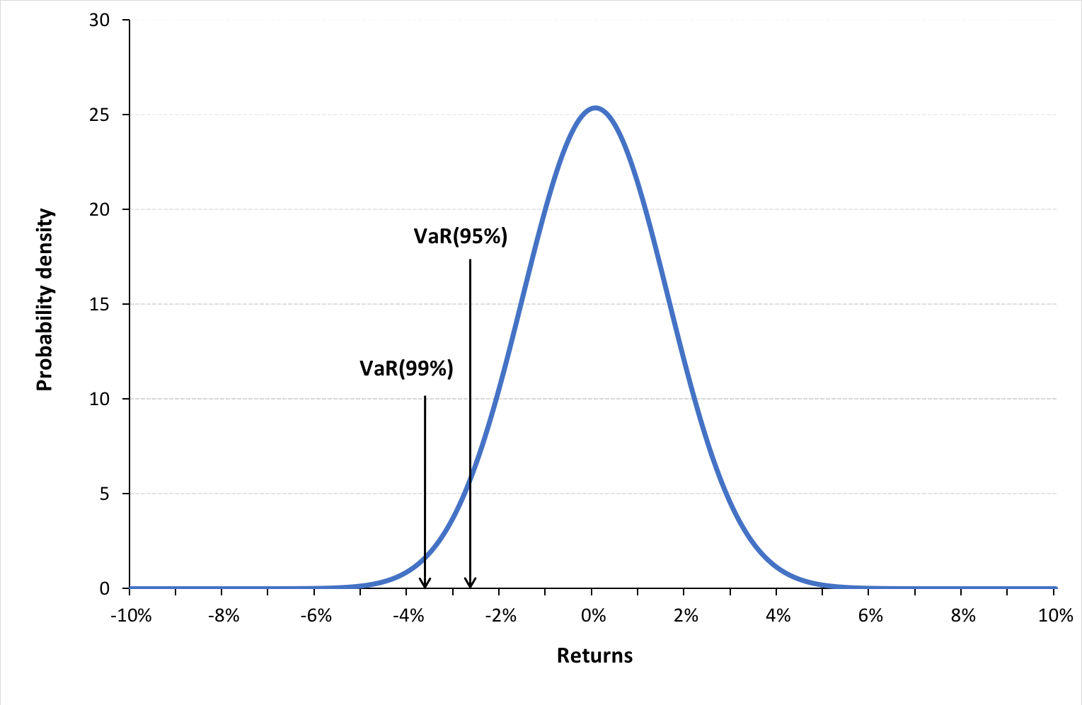
The variance-covariance method assumes that asset returns are normally distributed around the mean of the bell-shaped probability distribution. Assets may have tendency to move up and down together or against each other. This method assumes that the standard deviation of asset returns and the correlations between asset returns are constant over time.

VaR for single asset

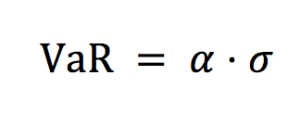
VaR calculation for a single asset is straightforward. From the distribution of returns calculated from daily price series, the standard deviation (σ) under a certain time horizon is estimated. The daily VaR is simply a function of the standard deviation and the desired confidence level and can be expressed as:

img_VaR_single_asset

Where the parameter ɑ links the quantile of the normal distribution and the standard deviation: ɑ = 2.33 for p = 99% and ɑ = 1.645 for p = 90%.

In practice, the variance (and then the standard deviation) is estimated from historical data.
img_VaR_asset_variance

Where R_t is the return on period [t-1, t] and R the average return.

Figure 1. Normal distribution for VaR for the CAC40 index
Normal distribution VaR for the CAC40 index
Source: computation by the author (data source: Bloomberg).

You can download below the Excel file for the VaR calculation with the variance-covariance method. The two parameters of the normal distribution (the mean and standard deviation) are estimated with historical data from the CAC 40 index.

VaR for a portfolio of assets

Consider a portfolio P with N assets. The first step is to compute the variance-covariance matrix. The variance of returns for asset X can be expressed as:

Variance

To measure how assets vary with each other, we calculate the covariance. The covariance between returns of two assets X and Y can be expressed as:

Covariance

Where X_t and Y_t are returns for asset X and Y on period [t-1, t].

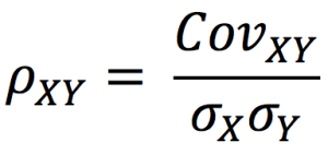
Next, we compute the correlation coefficients as:

img_correlation_coefficient

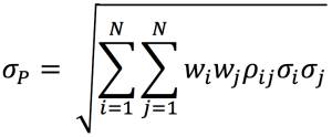
We calculation the standard deviation of portfolio P with the following formula:

img_VaR_std_dev_portfolio

img_VaR_std_dev_portfolio_2

Where w_i corresponds to portfolio weights of asset i.

Now we can estimate the VaR of our portfolio as:

img_portfolio_VaR

Where the parameter ɑ links the quantile of the normal distribution and the standard deviation: ɑ = 2.33 for p = 99% and ɑ = 1.65 for p = 95%.

Advantages and limitations of the variance-covariance method

Investors can estimate the probable loss value of their portfolios for different holding time periods and confidence levels. The variance–covariance approach helps us measure portfolio risk if returns are assumed to be distributed normally. However, the assumptions of return normality and constant covariances and correlations between assets in the portfolio may not hold true in real life.

Useful resources

Jorion P. (2007) Value at Risk, Third Edition, Chapter 10 – VaR Methods, 274-276.

About the author

The article was written in December 2021 by Jayati WALIA (ESSEC Business School, Grande Ecole Program – Master in Management, 2019-2022).

Standard deviation

December 9, 2021 by Jayati WALIA

Standard deviation

In this article, Jayati WALIA (ESSEC Business School, Grande Ecole Program – Master in Management, 2019-2022) presents an overview of standard deviation and its use in financial markets.

Mathematical formulae

To identify the center or average of any data set, measures of central tendency such as mean, median, mode and so on are used. These measures can be inherently used to represent any typical value in the particular data set. Considering a variable X, the arithmetic mean of a data set with N observations, X₁, X₂ … X_N, is computed as:

img_arithmetic_mean

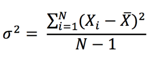
In the data set analysis, we also consider the dispersion or variability of data values around the central tendency or the mean. The variance of a data set is a measure of dispersion of data set values from the (estimated) mean and can be expressed as:

variance

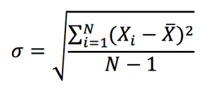
A problem with variance, however, is the difficulty of interpreting it due to its squared unit of measurement. This issue is resolved by using the standard deviation, which has the same measurement unit as the observations of the data set (such as percentage, dollar, etc.). The standard deviation is computed as the square root of variance:

standard deviation

A low value standard deviation indicates that the data set values tend to be closer to the mean of the set and thus lower dispersion, while a high standard deviation indicates that the values are spread out over a wider range indication higher dispersion.

Measure of volatility

For financial investments, the X variable in the above formulas would correspond to the return on the investment computed on a given period of time. We usually consider the trade-off between risk and reward. In this context, the reward corresponds to the expected return measured by the mean, and the risk corresponds to the standard deviation of returns.

In financial markets, the standard deviation of asset returns is used as a statistical measure of the risk associated with price fluctuations of any particular security or asset (such as stocks, bonds, etc.) or the risk of a portfolio of assets (such as mutual funds, index mutual funds or ETFs, etc.).

Investors always consider a mathematical basis to make investment decisions known as mean-variance optimization which enables them to make a meaningful comparison between the expected return and risk associated with any security. In other words, investors expect higher future returns on an investment on average if that investment holds a relatively higher level of risk or uncertainty. Standard deviation thus provides a quantified estimate of the risk or volatility of future returns.

In the context of financial securities, the higher the standard deviation, the greater is the dispersion between each return and the mean, which indicates a wider price range and hence greater volatility. Similarly, the lower the standard deviation, the lesser is the dispersion between each return and the mean, which indicates a narrower price range and hence lower volatility for the security.

Example: Apple Stock

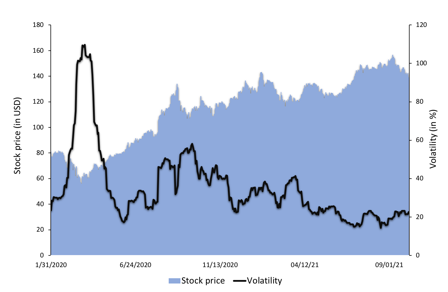
To illustrate the concept of volatility in financial markets, we use a data set of Apple stock prices. At each date, we compute the volatility as the standard deviation of daily stock returns over a rolling window corresponding to the past calendar month (about 22 trading days). This daily volatility is then annualized and expressed as a percentage.

Figure 1. Stock price and volatility of Apple stock.

price and volatility for Apple stock
Source: computation by the author (data source: Bloomberg).

You can download below the Excel file for the calculation of the volatility of stock returns. The data used are for Apple for the period 2020-2021.

Useful resources

Wikipedia Standard Deviation

About the author

The article was written in November 2021 by Jayati WALIA (ESSEC Business School, Grande Ecole Program – Master in Management, 2019-2022).

Systematic risk and specific risk

November 30, 2021 by Youssef LOURAOUI

In this article, Youssef LOURAOUI (Bayes Business School, MSc. Energy, Trade & Finance, 2021-2022) presents the systematic risk and specific risk of financial assets, two fundamental concepts in asset pricing models and investment management theories more generally.

This article is structured as follows: we introduce the concept of systematic and specific risk. We then explain the mathematical foundation of this concept. We finish with an insight that sheds light on the relationship between diversification and risk reduction.

Portfolio Theory and Risk

Markowitz (1952) and Sharpe (1964) developed a framework on risk based on their significant work in portfolio theory and capital market theory. All rational profit-maximizing investors seek to possess a diversified portfolio of risky assets, and they borrow or lend to get to a risk level that is compatible with their risk preferences under a set of assumptions. They demonstrated that the key risk measure for an individual asset is its covariance with the market portfolio under these circumstances (the beta).

The fraction of an individual asset’s total variance attributable to the variability of the total market portfolio is referred to as systematic risk, which is assessed by the asset’s covariance with the market portfolio. In the article systematic risk, we develop the economic sources of systematic risk: interest rate risk, inflation risk, exchange rate risk, geopolitical risk, and natural risk.

Additionally, due to the asset’s unique characteristics, an individual asset exhibits variance that is unrelated to the market portfolio (the asset’s non-market variance). Specific risk is the term for non-market variance, and it is often seen as minor because it can be eliminated in a large diversified portfolio. In the article specific risk, we develop the economic sources of specific risk: business risk and financial risk.

Mathematical foundations

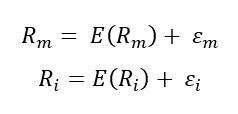
Following the Capital Asset Pricing Model (CAPM), the return on asset i, denoted by R_i can be decomposed as

img_SimTrade_return_decomposition

Where:

R_i the return of asset i
E(R_i) the expected return of asset i
β_i the measure of the risk of asset i
R_M the return of the market
E(R_M) the expected return of the market
R_M – E(R_M) the market factor
ε_i the specific part of the return of asset i

The three components of the decomposition are the expected return, the market factor and an idiosyncratic component related to asset only. As the expected return is known over the period, there are only two sources of risk: systematic risk (related to the market factor) and specific risk (related to the idiosyncratic component).

The beta of the asset with the market is computed as:

Beta

Where:

σ_i,m : the covariance of the asset return with the market return
σ_m² : the variance of market return

Total risk can be deconstructed into two main blocks:

Total risk formula

The total risk of the asset measured by the variance of asset returns can be computed as:

Decomposition of total risk

Where:

β_i² * σ_m² = systematic risk
σ_εi² = specific risk

In this decomposition of the total variance, the first component corresponds to the systematic risk and the second component to the specific risk.

Effect of diversification on portfolio risk

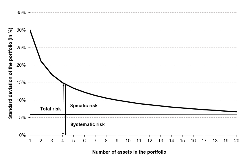
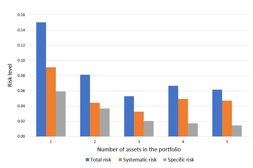
Diversification’s objective is to reduce the portfolio’s standard deviation. This assumes an imperfect correlation between securities. Ideally, as investors add securities, the portfolio’s average covariance decreases. How many securities must be included to create a portfolio that is completely diversified? To determine the answer, investors must observe what happens as the portfolio’s sample size increases by adding securities with some positive correlation. Figure 1 illustrates the effect of diversification on portfolio risk, more precisely on total risk and its two components (systematic risk and specific risk).

Figure 1. Effect of diversification on portfolio risk

Source: Computations from the author.

The critical point is that by adding stocks that are not perfectly correlated with those already held, investors can reduce the portfolio’s overall standard deviation, which will eventually equal that of the market portfolio. At that point, investors eliminated all specific risk but retained market or systematic risk. There is no way to completely eliminate the volatility and uncertainty associated with macroeconomic factors that affect all risky assets. Additionally, investors can reduce systematic risk by diversifying globally rather than just within the United States, as some systematic risk factors in the United States market (for example, US monetary policy) are not perfectly correlated with systematic risk variables in other countries such as Germany and Japan. As a result, global diversification eventually reduces risk to a global systematic risk level.

You can download below two Excel files which illustrate the effect of diversification on portfolio risk.

The first Excel file deals with the case of independent assets with the same profile (risk and expected return).

Figure 2 depicts the risk reduction of total risk in as we increase the number of assets in the portfolio. We manage to reduce half of the overall portfolio volatility by adding five assets to the portfolio. However, the decrease becomes more and more marginal as we add more assets.

Figure 2. Risk reduction of the portfolio. img_SimTrade_systematic_specific_risk_1 Source: Computations from the author.

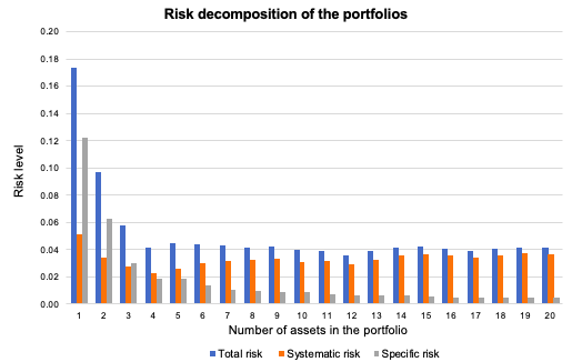
Figure 3 depicts the overall risk reduction of a portfolio. The benefit of diversification are more evident when we add the first 5 assets in the portfolio. As depicted in Figure 2, the diversification starts to fade at a certain point as we keep adding more assets in the portfolio. It can be seen in this figure how the specific risk is considerably reduced as we add more assets because of the effect of diversification. Systematic risk (market risk) is more constant and doesn’t change drastically as we diversify the portfolio. Overall, we can clearly see that diversification helps decrease the total risk of a portfolio considerably.

Figure 3. Risk decomposition of the portfolio. img_SimTrade_systematic_specific_risk_2 Source: Computations from the author.

The second Excel file deals with the case of dependent assets with the different characteristics (expected return, volatility, and market beta).

Academic research

A series of studies examined the average standard deviation for a variety of portfolios of randomly chosen stocks with varying sample sizes. Evans and Archer (1968) and Tole (1982) calculated the standard deviation for portfolios up to a maximum of twenty stocks. The results indicated that the majority of the benefits of diversification were obtained relatively quickly, with approximately 90% of the maximum benefit of diversification being obtained from portfolios of 12 to 18 stocks. Figure 1 illustrates this effect graphically.

This finding has been modified in two subsequent studies. Statman (1987) examined the trade-off between diversification benefits and the additional transaction costs associated with portfolio expansion. He concluded that a portfolio that is sufficiently diversified should contain at least 30–40 stocks. Campbell, Lettau, Malkiel, and Xu (2001) demonstrated that as the idiosyncratic component of an individual stock’s total risk (specific risk) has increased in recent years, it now requires a portfolio to contain more stocks to achieve the same level of diversification. For example, they demonstrated that the level of diversification possible in the 1960s with only 20 stocks would require approximately 50 stocks by the late 1990s (Reilly and Brown, 2012).

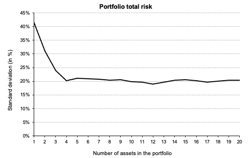
Figure 4. Effect of diversification on portfolio risk Source: Computation from the author.

You can download below the Excel file which illustrates the effect of diversification on portfolio risk with real assets (Apple, Microsoft, Amazon, etc.). The effect of diversification on the total risk of the portfolio is already significant with the addition of few stocks.

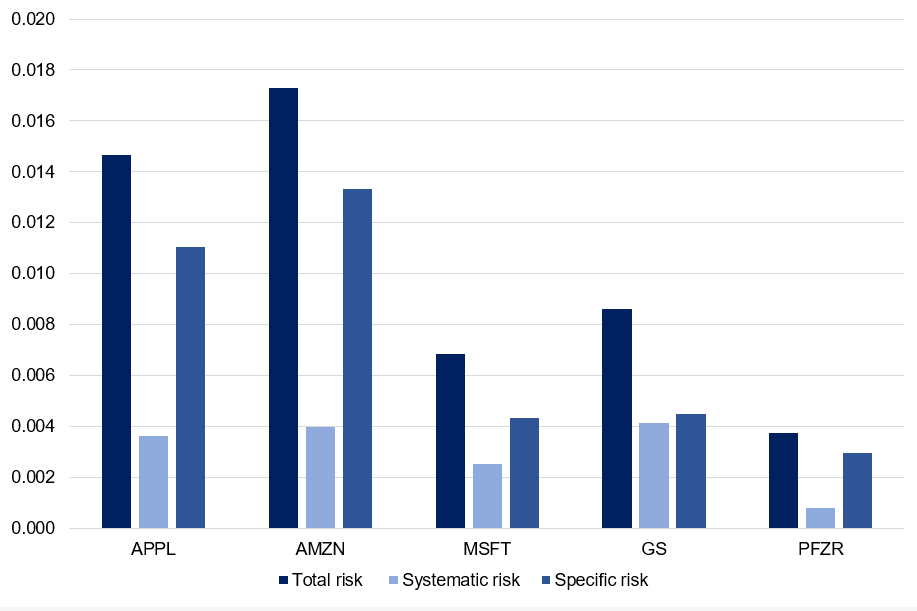
We can appreciate the decomposition of total risk in the below figure with real asset. We can appreciate how asset with low beta had the lowest systematic out of the sample analyzed (i.e. Pfizer). For the whole sample, specific risk is a major concern which makes the major component of risk of each stock. This can be mitigated by holding a well-diversified portfolio that can mitigate this component of risk. Figure 5 depicts the decomposition of total risk for assets (Apple, Microsoft, Amazon, Goldman Sachs and Pfizer).

Figure 5. Decomposition of total risk Source: Computation from the author.

You can download below the Excel file which deconstructs the risk of assets (Apple, Microsoft, Amazon, Goldman Sachs, and Pfizer).

Why should I be interested in this post?

If you’re an investor, understanding the source of risk is essential in order to build balanced portfolios that can withstand market corrections and downturns.

If you are a business school or university undergraduate or graduate student, this content will help you in broadening your knowledge of finance.

Useful resources

Academic research

Campbell, J.Y., Lettau, M., Malkiel, B.G. and Xu, Y. 2001. Have Individual Stocks Become More Volatile? An Empirical Exploration of Idiosyncratic Risk. The Journal of Finance, 56: 1-43.

Evans, J.L., Archer, S.H. 1968. Diversification and the Reduction of Dispersion: An Empirical Analysis. The Journal of Finance, 23(5): 761–767.

Markowitz, H. 1952. Portfolio Selection. The Journal of Finance, 7(1): 77-91.

Mossin, J. 1966. Equilibrium in a Capital Asset Market. Econometrica, 34(4): 768-783.

Reilly, R.K., Brown C.K. 2012. Investment Analysis & Portfolio Management, Tenth Edition. 239-245.

Sharpe, W.F. 1963. A Simplified Model for Portfolio Analysis. Management Science, 9(2): 277-293.

Sharpe, W.F. 1964. Capital Asset Prices: A Theory of Market Equilibrium under Conditions of Risk. The Journal of Finance, 19(3): 425-442.

Statman, M. 1987. How Many Stocks Make a Diversified Portfolio?. The Journal of Financial and Quantitative Analysis, 22(3), 353–363.

Tole T.M. 1982. You can’t diversify without diversifying. The Journal of Portfolio Management. Jan 1982, 8 (2) 5-11.

About the author

The article was written in November 2021 by Youssef LOURAOUI (Bayes Business School, MSc. Energy, Trade & Finance, 2021-2022).

Security Market Line (SML)

November 20, 2021 by Youssef LOURAOUI

In this article, Youssef LOURAOUI (Bayes Business School, MSc. Energy, Trade & Finance, 2021-2022) presents the Security Market Line (SML), a key concept in asset pricing derived from the Capital Asset Pricing Model (CAPM).

This article is structured as follows: we first introduce the concept of Security Market Line (SML). We then present the mathematical foundations of the SML. We finish by presenting an investment strategy that can be implemented relying on the SML.

Security Market Line

The SML reflects the risk-return combinations accessible in the capital market at any given time for all risky assets. Investors would choose investments based on their risk appetites; some would only consider low-risk investments, while others would welcome high-risk investments. The SML is derived from the Capital Asset Pricing Model (CAPM), which describes the trade-off between risk and expected return for efficient portfolios.

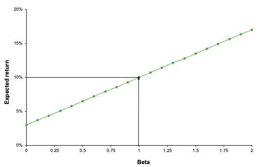
The expected relationship between risk and return is depicted in Figure 1. It demonstrates that as perceived risk increases, investors’ required rates of return increase.

Figure 1. Security Market Line.

Source: Computation by the author.

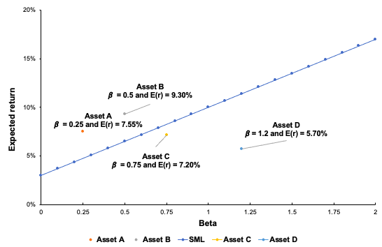
Under the CAPM framework, all investors will choose a position on the capital market line by borrowing or lending at the risk-free rate, since this maximizes the return for a given level of risk. Whereas the CML indicates the rates of return of a specific portfolio, the SML represents the risk and return of the market at a given point in time and indicates the expected returns of individual assets. Also, while the measure of risk in the CML is the standard deviation of returns (total risk), the measure of risk in the SML is the systematic risk, or beta. Figure 2 depicts the SML line combined with four different assets. Asset A and B are above the SML line, which implies that they are overvalued. Asset C and D are below the SML which implies that they are undervalued. From Figure 2, we can implement an investment strategy by going long if the asset or portfolio lies under the SML and going short if the asset or portfolio is greater than the SML.

Figure 2. Security Market Line with a plot of different assets.

Source: Computation by the author.

Mathematical foundation

The SML plots an individual security’s expected rate of return against systematic, undiversifiable risk. The risk associated with an individual risky security is determined by the volatility of the security’s return, not by the market portfolio’s return. Individual risky securities bear a proportional share of the systematic risk. The only risk that an investor should be compensated for is systematic risk, which cannot be neutralized through diversification. This risk is quantified using the beta, which refers to a security’s sensitivity to market fluctuations. The slope of the SML is equal to the market risk premium and reflects the risk-reward trade-off at a particular point in time. We can define the line of the SML as:

Mathematically, we can deconstruct the SML as:

SML_formula

Where

E(R_i) represents the expected return of asset i
R_f is the risk-free interest rate
β_i measures the systematic risk of asset i
E(R_M) represents the expected return of the market
E[R_M – R_f] represents the market risk premium.

Beta and the market factor

William Sharpe (1964), John Lintner (1965), and Jan Mossin (1966) independently developed the Capital Asset Pricing Model (CAPM). The CAPM was a significant evolutionary step forward in capital market equilibrium theory because it allowed investors to value assets correctly in terms of risk. The CAPM makes a distinction between two forms of risk: systematic and specific risk. Systematic risk refers to the risk posed by the market’s basic structure, its participants, and all non-diversifiable elements such as monetary policy, political events, and natural disasters. By contrast, specific risk refers to the risk inherent in a particular asset and so is diversifiable. As a result, the CAPM solely captures systematic risk via the beta measure, with the market’s beta equal to one, lower-risk assets having a beta less than one, and higher-risk assets having a beta larger than one.

In the late 1970s, the portfolio management industry sought to replicate the market portfolio return, but as financial research advanced and significant contributions were made, it enabled the development of additional factor characteristics to capture additional performance. This resulted in the development of what is now known as factor investing.

Estimation of the Security Market Line

You can download an Excel file with data to estimate the Security Market Line.

Why should I be interested in this post?

The security market line is frequently used by portfolio managers and investors to determine the suitability of an investment product for inclusion in a portfolio. The SML is useful for determining whether a security’s expected return is favourable in comparison to its level of risk. The SML is frequently used to compare two similar securities that offer approximately the same rate of return to determine which one has the lowest inherent market risk in relation to the expected rate of return. Additionally, the SML can be used to compare securities of comparable risk to determine which one offers the highest expected return for that level of risk.

If you are a business school or university undergraduate or graduate student, this content will help you in broadening your knowledge of finance.

Useful resources

Academic research

Drake, P. and Fabozzi, F., 2010. The Basics of Finance: An Introduction to Financial Markets, Business Finance, and Portfolio Management. John Wiley and Sons Edition.

Lintner, J. 1965a. The Valuation of Risk Assets and the Selection of Risky Investments in Stock Portfolios and Capital Budgets. The Review of Economics and Statistics 47(1): 13-37.

Lintner, J. 1965b. Security Prices, Risk and Maximal Gains from Diversification. The Journal of Finance, 20(4): 587-615.

Mossin, J. 1966. Equilibrium in a Capital Asset Market. Econometrica, 34(4): 768-783.

Reilly, R. K., Brown C. K., 2012. Investment Analysis & Portfolio Management, Tenth Edition.

Sharpe, W.F. 1963. A Simplified Model for Portfolio Analysis. Management Science, 9(2): 277-293.

Sharpe, W.F. 1964. Capital Asset Prices: A Theory of Market Equilibrium under Conditions of Risk. The Journal of Finance, 19(3): 425-442.

About the author

The article was written in November 2021 by Youssef LOURAOUI (Bayes Business School, MSc. Energy, Trade & Finance, 2021-2022).

VIX index

September 12, 2021 by Youssef LOURAOUI

VIX index

In this article, Youssef LOURAOUI (ESSEC Business School, Global Bachelor of Business Administration, 2017-2021) presents the VIX index, which is a financial index that measures the uncertainty in the US equity market.

This article is structured as follows: we begin by defining the grounding notions of the VIX index. We then explain the behavior of this index and its statistical characteristics. We finish by presenting its practical usage in financial markets.

Definition

The CBOE Volatility Index, abbreviated “VIX”, is a measure of the expected S&P 500 index movement calculated by the Chicago Board Options Exchange (CBOE) from the current trading prices of options written on the S&P 500 index.

Known as Wall Street’s “fear index”, the VIX is closely monitored by a broad range of market players, and its level and pattern have become ingrained in market discussion.

Figure 1 illustrates the evolution of the VIX index for the period from 2003 to 2021.
Figure 1 Historical levels of the VIX index from 2003-2021.

Source: computation by the author (Data source: Thomson Reuters).

VIX values greater than 20 are regarded to be high by market participants. If the VIX is between 12 and 20, it is considered normal; if it is less than 12, it is considered low. As it is the case with other indices, the VIX is computed using the price of a basket of tradable components (in this case, options expiring within the next month or so). The profit or loss that option buyers and sellers realize during the option’s life will depend, among other things, on how significantly the S&P 500’s actual volatility will differ from the implied volatility given by the VIX at the start of the period (S&P Global Research, 2017).

Behavior of the VIX index

Statistical distribution of the S&P500 index returns and VIX level

Figure 2 displays the statistical distribution of the price variations in the S&P500 index for different levels of the VIX index The higher the VIX index (by convention, greater than 20), the more severe the distribution tends to be, with negative skewness and high kurtosis indicating heightened volatility in the US market, therefore exacerbating both positive and negative swings. An opposite finding may be made for the VIX level at lower levels (often less than 12), when market swings are less evident due to less skewness and lower kurtosis (S&P Global Research, 2017).

Figure 2. The distribution of 30-day return in the S&P500 index for different VIX index levels.

Source: S&P Global Research (2017).

If the VIX is low, market players may benefit by purchasing options; conversely, if the VIX is high, market participants may profit from selling options. The specific utility of anticipated VIX is that it gives us with a more accurate assessment of whether VIX is high, low, or normal at any point in time (S&P Global Research, 2017). Thus, VIX may be regarded of as a crowd-sourced estimate of the S&P 500’s expected volatility. As with interest rates and dividends, one cannot invest directly in them, even though one can guess on their future worth, one cannot invest directly in VIX, and the significance of a specific VIX level is commonly misinterpreted (S&P Global Research, 2017).

Recent volatility in the S&P500 index and VIX level

Figure 3 demonstrates that the VIX index is strongly correlated with recent market volatility. However, there is considerable variance; for example, a recent volatility level of about 20% has been associated with a VIX level of 34 (point B, when VIX was very “high”) and with a VIX level of 12 (point C, when VIX was relatively “low”). Volatility (realized or implied) has a strong propensity to return to its mean. This insight is not especially original, despite its illustrious past. There is an enormous body of data demonstrating that volatility tends to mean revert across markets, and the pioneers of this field were given the Nobel Prize in part for incorporating their results into volatility forecasts and simulations (S&P Global Research, 2017).

Figure 3. Relation between VIX and recent volatility.

Source: S&P Global Research (2017).

Realized volatility in the S&P500 index and VIX level

Figure 4 represents the relationship between Realized volatility in the S&P500 index over a period and the VIX level at the begining of the period.

Figure 4. VIX versus next realized volatility.

Source: S&P Global Research (2017).

Mean reversion

Figure 5 shows how VIX index converge to a certain llong-term level as time passes. This finding is not due to 15% being exceptional in any manner; this figure for M was calculated using historical volatility levels for the S&P 500 and their evolution. It is not implausible that M (else referred to as long-term average volatility in the US equities market) may change over time; changes in the S&P 500’s sector weightings, trade All of these factors have the ability to influence both the pace and the volume and the point at which mean reversion occurs.

Figure 5. Mean-reversion dynamic in recent volatility.

Source: S&P Global Research (2017).

Use of the VIX index in financial markets

There are two methods for determining an asset’s volatility. Either through a statistical calculation of an asset’s realized volatility, also known as historical volatility, which serves as a pointer to the asset’s volatility behavior. This is a limited method that is based on the premise that past volatility tends to replicate itself in the future, without including a forward-looking study of volatility. The second technique is to extract an asset’s volatility from option prices referred to as “implied volatility”.

Why should I be interested in this post?

When investors make investment decisions, they utilize the VIX to gauge the degree of risk, worry, or stress in the market. Additionally, traders can trade the VIX using a range of options and exchange-traded products, or price derivatives using VIX values.

Useful resources

Business analysis

CBOE , 2021. VIX

Nasdaq, 2021. Realized Volatility

Nasdaq, 2021. Vix Index Volatility

S&P Global Research, 2017. Reading VIX: Does VIX Predict Future Volatility?

S&P Global Research, 2017. A Practitioner’s Guide to Reading VIX

About the author

The article was written in September 2021 by Youssef LOURAOUI (ESSEC Business School, Global Bachelor of Business Administration, 2017-2021).

Value at Risk

August 24, 2021 by Jayati WALIA

Value at Risk

In this article, Jayati WALIA (ESSEC Business School, Grande Ecole Program – Master in Management, 2019-2022) presents value at risk.

Introduction

Risk Management is a fundamental pillar of any financial institution to safeguard the investments and hedge against potential losses. The key factor that forms the backbone for any risk management strategy is the measure of those potential losses that an institution is exposed to for any investment. Various risk measures are used for this purpose and Value at Risk (VaR) is the most commonly used risk measure to quantify the level of risk and implement risk management.

VaR is typically defined as the maximum loss which should not be exceeded during a specific time period with a given probability level (or ‘confidence level’). Investments banks, commercial banks and other financial institutions extensively use VaR to determine the level of risk exposure of their investment and calculate the extent of potential losses. Thus, VaR attempts to measure the risk of unexpected changes in prices (or return rates) within a given period.

Mathematically, the VaR corresponds to the quantile of the distribution of returns on the investment.

VaR was not widely used prior to the mid 1990s, although its origin lies further back in time. In the aftermath of events involving the use of derivatives and leverage resulting in disastrous losses in the 1990s (like the failure of Barings bank), financial institutions looked for better comprehensive risk measures that could be implemented. In the last decade, VaR has become the standard measure of risk exposure in financial service firms and has even begun to find acceptance in non-financial service firms.

Computational methods

The three key elements of VaR are the specified level of loss, a fixed period of time over which risk is assessed, and a confidence interval which is essentially the probability of the occurrence of loss-causing event. The VaR can be computed for an individual asset, a portfolio of assets or for the entire financial institution. We detail below the methods used to compute the VaR.

Parametric methods

The most usual parametric method is the variance-covariance method based on the normal distribution.

In this method it is assumed that the price returns for any given asset in the position (and then the position itself) follow a normal distribution. Using the variance-covariance matrix of asset returns and the weights of the assets in the position, we can compute the standard deviation of the position returns denoted as σ. The VaR of the position can then simply computed as a function of the standard deviation and the desired probability level.

VaR Formula

Wherein, p represents the probability used to compute the VaR. For instance, if p is equal to 95%, then the VaR corresponds to the 5% quantile of the distribution of returns. We interpret the VaR as a measure of the loss we observe in 5 out of every 100 trading periods. N^-1(x) is the inverse of the cumulative normal distribution function of the confidence level x.

Figure 1. VaR computed with the normal distribution.

VaR computed with the normal distribution

For a portfolio with several assets, the standard deviation is computed using the variance-covariance matrix. The expected return on a portfolio of assets is the market-weighted average of the expected returns on the individual assets in the portfolio. For instance, if a portfolio P contains assets A and B with weights w_A and w_B respectively, the variance of portfolio P’s returns would be:

Variance of portfolio

In the variance-covariance method, the volatility can be computed as the unconditional standard deviation of returns or can be calculated using more sophisticated models to consider the time-varying properties of volatility (like a simple moving average (SMA) or an exponentially weighted moving average (EWMA)).

The historical distribution

In this method, the historical data of past returns (for say 1,000 daily returns or 4 years of data) are used to build an historical distribution. VaR corresponds to the (1-p) quantile of the historical distribution of returns.
This methodology is based on the approach that the pattern of historical returns is indicative of future returns. VaR is estimated directly from data without estimating any other parameters hence, it is a non-parametric method.

Figure 2. VaR computed with the historical distribution.

VaR computed with the historical distribution

Monte Carlo Simulations

This method involves developing a model for generating future price returns and running multiple hypothetical trials through the model. The Monte Carlo simulation is the algorithm through which trials are generated randomly. The computation of VaR is similar to that in historical simulations. The difference only lies in the generation of future return which in case of the historical method is based on empirical data while it is based on simulated data in case of the Monte Carlo method.

The Monte Carlo simulation method is used for complex positions like derivatives where different risk factors (price, volatility, interest rate, dividends, etc.) must be considered.

Limitations of VaR

VaR doesn’t measure worst-case loss

VaR gives a percentage of loss that can be faced in a given confidence level, but it does not tell us about the amount of loss that can be incurred beyond the confidence level.

VaR is not additive

The combined VaR of two different portfolios may be higher than the sum of their individual VaRs.

VaR is only as good as its assumptions and input parameters

In VaR calculations especially parametric methods, unrealistic or inaccurate inputs can give misleading results for VaR. For instance, using the variance-covariance VaR method by assuming normal distribution of returns for assets and portfolios with non-normal skewness.

Different methods give different results

There are many approaches that have been defined over the years to estimate VaR. However, it essential to be careful in choosing the methodology keeping in mind the situation and characteristics of the portfolio or asset into consideration as different methods may be more accurate for specific scenarios.

Useful Resources

Academic research articles

Artzner, P., F. Delbaen, J.-M. Eber, and D. Heath, (1999) Coherent Measures of Risk, Mathematical Finance, 9, 203-228.

Jorion P. (1997) “Value at Risk: The New Benchmark for Controlling Market Risk,” Chicago: The McGraw-Hill Company.

Longin F. (2000) From VaR to stress testing: the extreme value approach Journal of Banking and Finance, N°24, pp 1097-1130.

Longin F. (2016) Extreme events in finance: a handbook of extreme value theory and its applications Wiley Editions.

Longin F. (2001) Beyond the VaR Journal of Derivatives, 8, 36-48.

About the author

The article was written in September 2021 by Jayati WALIA (ESSEC Business School, Grande Ecole Program – Master in Management, 2019-2022).

Plain Vanilla Options

June 4, 2024August 23, 2021 by Jayati WALIA

Plain Vanilla Options

In this article, Jayati WALIA (ESSEC Business School, Grande Ecole Program – Master in Management, 2019-2022) presents plain vanilla options.

Introduction

An option contract is a financial derivative that gives its holder the right (but not the obligation) to trade an underlying asset at a price and a date set in advance.

In finance, plain vanilla refers to the most basic version of any financial instrument with standard features. Thus, a plain vanilla option simply refers to a contract that provides the option to buy or sell an underlying stock (or any financial asset) at a fixed price (known as the exercise/strike price) at an expiration date in the future. The expiration date (or maturity) of the option is the date when the holder can exercise her option if she wants.

In the US, options were first traded on an exchange on 26th April 1973. The Chicago Board Options Exchange (CBOE) was the first to create standardized, listed options. Today, there are over 50 exchanges worldwide that trade options.

When an option is bought, its holder pays a fixed amount to the option writer as the cost for the flexibility of trading that the option provides. This cost, which is essentially the value of an option (and the margin taken by the issuer), is known as the premium. The premium depends on the characteristics of the option like the strike price and the maturity, and on market data like the price of the underlying asset and especially its volatility. Many different underlying assets can be traded through options including stocks, bonds, commodities, foreign currencies.

Types of options

Vanilla options are of two types: call and put.

Call options

The holder of a call option has the right to buy a particular asset at a strike price K at maturity T. If the asset price at maturity denoted by S_T is higher than K, then it is beneficial for the call option holder to exercise his option at time T as the price set in the call option contract K is lower than the market price S_T. If the asset price at maturity S_T is lower than K, then it is not beneficial for the call option holder to exercise his option at time T as the price set in the call option contract K is higher than the market price S_T; he is then better off to buy the asset on the market at price S_T than at price K.

For example, consider a call option on BNP Paribas stock with a strike price of €50 and a maturity date March 31^st. The holder of this call option thus has the right but not the obligation to buy one BNP Paribas stock for €50 at maturity. He will exercise his option on March 31^st if and only if the stock price is higher than €50.

The equation below gives the pay-off function of a call option that is the value of the call option at maturity T denoted by C_T as a function of the price of the underlying asset S_T.

Payoff formula for a call option

Figure 1 gives a graphical representation of the pay-off function of a call option that is the value of the call option at maturity T as a function of the price of the underlying asset at maturity T, S_T, for a given strike price (equal to €50 in the figure).

Figure 1. Pay-off function of a call option

Payoff for a call option

Put options

Similarly, the holder of a put option has the right to sell a particular asset at a strike price K at maturity T. If the asset price at maturity denoted by S_T is higher than K, then it is beneficial for the put option holder not to exercise his option at time T as the price set in the put option contract K is lower than the market price S_T; he is then better off to sell the asset on the market at price S_T than at price K. If the asset price at maturity S_T is lower than K, then it is beneficial for the put option holder to exercise his option at time T as the price set in the put option contract K is higher than the market price S_T.

For example, consider a put option on BNP Paribas stock with a strike price of €50 and a maturity date March 31^st. The holder of this put option thus has the right but not the obligation to sell one BNP Paribas stock for €50 at maturity. He will exercise his put option on March 31^st if and only if the stock price is lower than €50.

The equation below gives the pay-off function of a put option that is the value of the put option at maturity T denoted by P_T as a function of the price of the underlying asset S_T.

Payoff formula for a put option

Figure 2 gives a graphical representation of the pay-off function of a put option that is the value of the put option at maturity T as a function of the price of the underlying asset S_T for a given strike price (equal to €50 in the figure).

Figure 2. Pay-off function of a put option

Payoff for a put option

Types of exercise

Options can be categorized based on their exercise restrictions.

American options

American options have the most flexible arrangement allowing holders to exercise their options at any time prior to the expiration date. They are widely traded over listed exchanges.

European options

European options provide less flexibility and allow holders to exercise options on only one specific date, which is the expiration date. They thus have a lower value compared to American options and are generally traded OTC.

Bermudan options

There are also Bermudan options that allow exercise of options on a set of specific dates before the expiration and thus provide holders a level of flexibility midway between American and European Options.

Moneyness

Options can also be characterized by their “moneyness” which compares the current price of the underlying asset to the option strike.

In-the-money options

An option with a positive intrinsic value is said to be ‘in the money’. This is the case for a call option if the current market price of the asset is higher than the strike price, and similarly for a put option if the current market price of the asset is lower than the strike price.

Out-of-the-money options

An option with a zero intrinsic value is said to be ‘out of the money’. This is the case for a call option if the current market price of the asset is lower than the strike price, and similarly for a put option if the current market price of the asset is higher than the strike price.

At-the-money options

An option with a strike price close or equal to the current market price is said to be ‘at the money’.

Option writers

The above discussion mainly revolves around option purchasers. However, there is also someone who is liable to sell (for a call) or buy (for a put) the underlying security whenever any holder exercises an option. The writer of an option is the person who is obligated to buy/sell the underlying in case of a call/put exercise. As a counterpart, the writer also receives the option premium from the holder.

The best-case scenario for a writer would be that the option is not exercised by its holder as the option remains out of the money (the writer earning the premium without being obliged to pay the cash flow at maturity). However, option writers are exposed to downside risks especially if the options they write are not covered i.e., holding a long or short position already in the underlying security depending on the option written.

Benefits

For traders with strong market views looking to leverage benefits from small to medium-term fluctuations in market price, buying options is an efficient means to offset their risk exposure. The buyer only risks a small amount of investment, and the downside is only limited to the initial premium whereas the upside is a high payoff if the speculation is in her/his favor. The traders can also take up multiple positions in different assets through options and leverage trade opportunities with profitable positions covering more than the hedging costs.

Option Trading

Most vanilla options are traded through exchanges that make it convenient to match buyers with sellers and vice versa. Trading of standardized contracts also promotes liquidity of the instruments in the market. Vanilla options generally come in series of standardized strike prices and expiration dates. For instance, for an option contract on an Apple Inc. stock (AAPL) expiring on 20^th August 2021, the offered strike prices are $115, $120, $125, $130 and so on. Similarly, the expiration dates for listed stock options is generally the third Friday of the month in which the contract expires. If the Friday falls on a holiday, the expiration date becomes Thursday immediately before the third Friday.

Option pricing

The value an option is known at maturity as it is given by the contract. But what is the value of an option at the time of its issuance or at a time before maturity? Many mathematical models have been developed to answer this question. The most famous model is the Black-Scholes-Merton option pricing model. It uses a Brownian motion to model the behavior of stock market prices.

Use of options

Hedging

Options are commonly used in hedging. For instance, you can purchase an option on a stock to limit your losses to say 15% of your position, should the stock decline more than that during the option period.

Speculation

If one has a strong view about the potential market direction of an underlying security, one can make great returns on exploiting options, provided the view was right. This is essentially speculation in option trading. For instance, if you have a bullish opinion regarding a stock, you can purchase a call option on it that will allow you to purchase the stock at the strike price that will be lower than the future price (hopefully!). Thus, if you are right, you could exercise the option and your payoff would be the price difference between the stock price and the strike price. If you are wrong, you lose out on the premium you paid for the option.

Volatility

The volatility of the underlying asset affects positively option prices: stocks with higher volatility have more expensive option contracts that those with low volatility. In fact, the implied volatility (IV) of an option is that value of the volatility of the underlying instrument for which an option pricing model (such as the Black-Scholes-Merton model) will return a theoretical value equal to the current market price of that option. Hence, when the implied volatility increases, the price of options increases as well, assuming all other factors remain constant. When the implied volatility increases after a trade has been placed, it is good news for the option owner and, conversely bad news for the seller. Inversely, when the implied volatility decreases after a trade has been placed, it is bad news for the option owner and, conversely good news for the seller.

Note that the implied volatility tends to depend on the strike price and maturity date of the options for a given underlying asset. Once the implied volatility for the at-the-money contracts is determined in any given expiration month, market makers use pricing models and volatility skews to calculate implied volatility at other strike prices that are less heavily traded. So, every option has an associated volatility and risk profiles can vary drastically among options. Traders may at times balance out the risk of volatility by hedging one option with another.

Thus, it is essential to interpret and analyze risks before venturing into option trading. There are also many strategies that can be applied to vanilla options in order to benefit better and limit risk such as long and short calls/puts, bull and bear spreads, straddles and strangles, butterflies, condors among many.

Useful Resources

Nasdaq Historical data for Apple stock

AVATRADE What are vanilla options

TheStreet Options Trading

About the author

The article was written in August 2021 by Jayati WALIA (ESSEC Business School, Grande Ecole Program – Master in Management, 2019-2022).

Bond risks

May 30, 2021 by Rodolphe CHOLLAT-NAMY

Bond risks

In this article, Rodolphe CHOLLAT-NAMY (ESSEC Business School, Grande Ecole Program – Master in Management, 2019-2023) introduces you to bond risks.

Holding bonds exposes you to fluctuations in its price, both up and down. Nevertheless, bonds offer the guarantee of a coupon regularly paid during for a fixed period. Investing in bonds has long been considered one of the safest investments, especially if the securities are held to maturity. Nevertheless, a number of risks exist. What are these risks? How are they defined?

Default risk

Default risk is the risk that a company, local authority or government fails to pay the coupons or repay the face value of the bonds they issued. This risk can be low, moderate or high. It depends on the quality of the issuer.

For a given product, the default risk is mainly measured by rating agencies. Three agencies share 95% of the world’s rating requests. Moody’s and Standard & Poor’s (S&P) each hold 40% of the market, and Fitch Ratings 14%. The highest rated bonds (from Aaa to Baa3 at Moody’s and from AAA to BBB- at S&P and Fitch) are investment-grade bonds. The lowest rated bonds (Ba1 to Caa3 at Moody’s and BB+ to D at S&P and Fitch) are high yield bonds, otherwise known as junk bonds.

It should be noted that the opinions produced by an agency are advisory and indicative. Moreover, some criticisms have emerged. As agencies rate their clients, questions may be asked about their independence and therefore their impartiality. The analysis done aby rating agencies is most of the time paid by the entities that want their product to be rated.

In addition, companies issuing bonds are increasingly using the technique of “debt subordination”. This technique makes it possible to establish an order of priority between the different types of bonds issued by the same company, in the event that the company is unable to honor all its financial commitments. The order of priority is senior, mezzanine and junior debt. The higher the risk is, the higher the return is. It should also be noted that bonds have priority over equity.

To highlight the level of risk of an issuer, one can compare the yield of its bonds to those of a risk-free issuer. This is called the spread. Theoretically, it is the difference between the yield to maturity of a given bond and that of a zero-coupon bond with similar characteristics. The spread is usually measured in basis points (0.01%).

Liquidity risk

Liquidity risk is the degree of easiness in being able to buy or sell bonds in the secondary market quickly and at the desired price (i.e. with a limited price impact). If the market is illiquid, a bondholder who wishes to sell will have to agree to a substantial discount on the expected price in the best case, and will not be able to sell the bonds at all in the worst case.

The risk depends on the size of the issuance and the existence and functioning of the secondary market for the security. The liquidity of the secondary market varies from one currency to another and changes over time. In addition, a rating downgrade may affect the marketability of a security.

On the other hand, it may be an opportunity for investors who want to keep their illiquid bonds. Indeed, they usually get a better return. This is called the “liquidity premium”. It rewards the risk inherent in the investment and the unavailability of funds during this period.

Interest rate risk

The price of a bond fluctuates with interest rates. The price of a bond is inversely correlated to interest rates (the discount rate used to compute its present value). Indeed, the nominal interest rates follow the key rates. Thus, if rates rise, the coupons offered by new bonds will be higher than those offered by older bonds, issued with lower rates. Investors will therefore prefer the new bonds, which offer a better return, which will automatically lower the price of the older ones.

The interest rate risk is increasing with the maturity of the bond (more precisely its duration). The risk is low for bonds with a life of less than 3 years, moderate for bonds with a life of 3 to 5 years and high for bonds with a life of more than 5 years. However, interest rate risk does not impact investors who hold their bonds to maturity.

Inflation risk

Inflation presents a double risk to bondholders. Firstly, if inflation rises, the value of an investment in bonds will necessarily fall. For example, if an investor purchases a 5% fixed-rate bond, and inflation rises to 10% per year, the bondholder will lose money on the investment because the purchasing power of the proceeds has been greatly diminished. Secondly, high inflation can lead central banks to raise rates in order to tackle it, which, as we can see above, will depreciate the value of the bond.

To protect against this, some bonds, floating-rates bonds, are indexed to inflation. They guarantee their holders a daily readjustment of the value of their investment according to the evolution of inflation. However, these bonds have a cost in terms of return.

As with interest rate risk, the risk increases with the maturity of the bond. Also, the risk rises as the coupon decreases. The risk is therefore very high for zero-coupon bonds.

Currency risk

An investor can buy bonds in a currency other than its own. However, as with any investment in a foreign currency, the return on the bond will depend on the rate of that currency relative to the investor’s own currency.

For example, if an investor holds a $100 US bond. If the EUR/USD exchange rate is 1.30, the price of the bond will be €76.9. If the euro appreciates against the dollar and the exchange rate rises to 1.40, the price of the bond will be €71.4. Thus, the investor will lose money.

Useful resources

Rating agencies

S&P

Moody’s

Fitch Rating

▶ Rodolphe CHOLLAT-NAMY Bond valuation

▶ Rodolphe CHOLLAT-NAMY Bond markets

▶ Bijal GANDHI Credit Rating

▶ Jayati WALIA Credit risk

About the author

Article written in May 2021 by Rodolphe CHOLLAT-NAMY (ESSEC Business School, Grande Ecole Program – Master in Management, 2019-2023).

Risk comes from not knowing what you are doing

“Risk comes from not knowing what you are doing”

Analysis of the quote

About the author

Financial concepts related to the quote

Risk management

Due diligence

Portfolio diversification

My opinion about this quote

Why should I be interested in this post?

Related posts on the SimTrade blog

Useful resources

About the author

The Nikkei 225 index

The Nikkei 225 index

Calculation of the Nikkei 225 index value

Use of the Nikkei 225 index in asset management

Benchmark for equity funds

Financial products around the Nikkei 225 index

Historical data for the Nikkei 225 index

How to get the data?

R program

Data file

Evolution of the Nikkei 225 index

Summary statistics for the Nikkei 225 index

Statistical distribution of the Nikkei 225 index returns

Historical distribution

Gaussian distribution

Risk measures of the Nikkei 225 index returns

Financial maps

Why should I be interested in this post?

Related posts on the SimTrade blog

About financial indexes

Other financial indexes

About portfolio management

About statistics

Useful resources

Academic research about risk

Data

Other

About the author

Introduction

Computation methods for implied volatility

Example

Volatility smile

Volatility surface

CBOE Volatility Index

Related posts on the SimTrade blog

Useful resources

Academic articles

Business

About the author

Risk Aversion

Risk aversion and investor’s characteristics

Age

Income

Past Losses

Investment Objective

Investment Horizon

Risk aversion and financial investments

Measure of risk of financial assets

Standard Deviation

Beta

Modern Portfolio Theory & Risk

Risk aversion and economic conditions

Related posts

Useful resources

About the author

The incredible story of Nick Leeson & the Barings Bank

History of Barings and Nick Leeson’s background

The great fraud

Conclusion

Useful resources

Related posts on the SimTrade blog

About the author

What happened between Bruno Iksil & JP Morgan

Bruno Iksil: background of a French trader based in London

Iksil’s activities at JP Morgan

JP Morgan’s losses

Conclusion and aftermath of the affair