

In this article, Jayati WALIA (ESSEC Business School, Grande Ecole – Master in Management, 2019-2022) explains the Monte Carlo simulation method and its applications in finance.
Introduction
Monte Carlo simulations are a broad class of computational algorithms that rely majorly on repeated random sampling to obtain numerical results. The underlying concept is to model the multiple possible outcomes of an uncertain event. It is a technique used to understand the impact of risk and uncertainty in prediction and forecasting models.
The Monte Carlo method was invented by John von Neumann (Hungarian-American mathematician and computer scientist) and Stanislaw Ulam (Polish mathematician) during World War II to improve decision making under uncertain conditions. It is named after the popular gambling destination Monte Carlo, located in Monaco and home to many famous casinos. This is because the random outcomes in the Monte Carlo modeling technique can be compared to games like roulette, dice and slot machines. In his autobiography, ‘Adventures of a Mathematician’, Ulam mentions that the method was named in honor of his uncle, who was a gambler.
How Monte Carlo simulation works
The main idea is to repeatedly run a large number of simulations of a random process for a variable of interest (such as an asset price in finance) covering a wide range of possible situations. The outcomes of this variables are drawn from a pre-specified probability distribution that is assumed to be known, including the analytical function and its parameters. Thus, Monte Carlo simulations inherently try to recreate the entire distribution of asset prices.
Example: Apple stock
Consider the Apple stock as our asset of interest for which we will generate stock prices according to the Monte Carlo simulation method.
The first step in the simulation is choosing a stochastic model for the behavior of our random variable (the Apple stock price in our case). A commonly used model is the geometric Brownian motion (GBM) model. The model assumes that future asset price changes are uncorrelated over time and the probability distribution function of the future price is a log-normal distribution. The movements in price in GBM process can be expressed as:
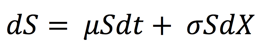
with dS being the change in asset price in continuous time dt. dW is the Wiener process (Wt+1 – Wt is a random variable from the normal distribution N(0, 1)). σ represents the price volatility considering the unexpected changes that can result from external effects (σ is assumed to be constant over time). μdt together represents the deterministic return within the time interval with μ representing the growth rate of the asset price or the ‘drift’.
Integrating dS/S over a finite interval, we get :
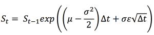
Where ε is a random number generated from a normal distribution N(0,1).
This equation thus gives us the evolution of the asset price from a simulated model from day t-1 to day t.
We can now generate a simulation path for 100 days using the above formula.
The figure below shows five simulations for the price of the Apple stock over 100 days with Δt = 1 day. The initial price for Apple stock (i.e, price at t=0) is $146.52.
Figure 1. Simulated Apple stock prices according to the Monte Carlo simulation method.
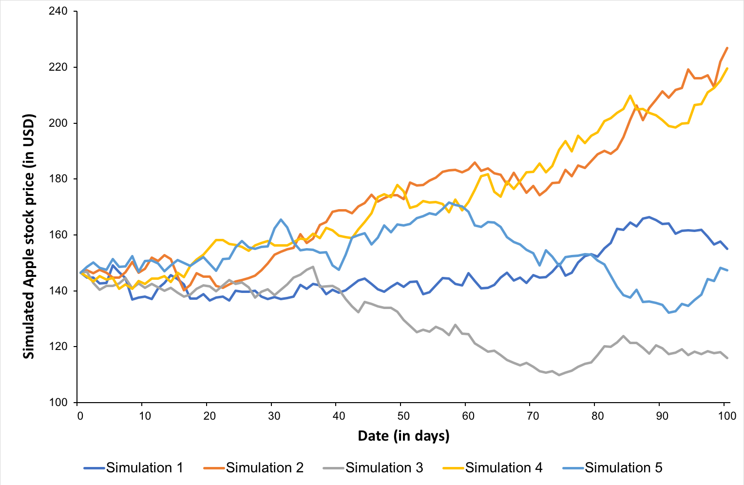
Source: computation by author.
Thus, we can observe that the prices obtained by just these five simulations range from $100 to over $220.
You can download below the Excel file for generating Monte Carlo Simulations for Apple stock.

Applications in finance
The Monte Carlo simulation method is widely used in finance for valuation and risk analysis purposes.
One popular application is option pricing. For option contracts with complicated features (such as Asian options) or those with a combination of assets as their underlying, Monte Carlo simulations help generate multiple potential payoff scenarios for the option which are averaged out to determine the option price at the issuance date.
The Monte Carlo method is also used to assess potential risks by generating simulations of market variables affecting portfolios such as asset returns, interest rates, macroeconomic factors, etc. over different time periods. These simulations are then assessed as required for risk modelling and to compute risk metrics such as the value at Risk (VaR) of a position.
Other applications include personal finance planning and corporate project finance where simulations are generated to construct stochastic financial models for sensitivity analysis and net present value (NPV) projections.
Related posts on the SimTrade blog
▶ Jayati WALIA Quantitative Risk Management
▶ Jayati WALIA Brownian Motion in Finance
▶ Jayati WALIA The Monte Carlo simulation method for VaR calculation
▶ Shengyu ZHENG Pricing barrier options with simulations and sensitivity analysis with Greeks
Useful resources
Hull, J.(2008) Risk Management and Financial Institutions, Fifth Edition, Chapter 7 – Valuation and Scenario Analysis.
About the author
The article was written in March 2022 by Jayati WALIA (ESSEC Business School, Grande Ecole Program – Master in Management, 2019-2022).