In this article, Marco SIMONETTI (ESSEC Business School, MSc in Finance, 2025-2027) shares his experience as an Off-Cycle Sales & Trading Derivatives Intern at Banca Monte dei Paschi di Siena in Milan. The internship gave me direct exposure to how a corporate and investment banking desk transforms market information into practical hedging and trading solutions for corporate clients.
My role sits at the intersection of markets, corporate finance and client advisory. On one side, I follow macroeconomic and market developments in real time; on the other, I help translate those developments into concrete ideas for clients exposed to commodities, foreign exchange and interest rates.
About the company
Banca Monte dei Paschi di Siena (MPS) is one of the major Italian banking groups and is widely known as the world’s oldest bank still in operation, with origins in Siena in 1472. Today, the Group operates across retail banking, corporate banking, wealth management and capital markets activities.
My internship is based in Milan, within Sales & Trading Derivatives. The desk works with corporate clients that are exposed to fluctuations in commodity prices, exchange rates and interest rates. For example, an industrial company may need to hedge the cost of energy or raw materials, while an exporter may need to manage the risk that currencies move against its future revenues.
The value added by this type of desk is not simply to sell a financial product. It is to understand the client’s business model, identify the risk exposure, structure an appropriate solution and coordinate with traders to deliver an executable price. In other words, the role combines technical knowledge, market timing and commercial judgment.
Logo of the company.
![]()
Source: Banca Monte dei Paschi di Siena.
My experience as a Sales & Trading Derivatives Intern
My missions
Client coverage and needs identification: I supported the coverage of a portfolio of around 20 clients, helping identify hedging and trading needs across commodities, foreign exchange (FX) and interest rates. In practice, this meant understanding what each company buys, sells, imports, exports or finances, and how market volatility can affect its margins, cash flows and planning.
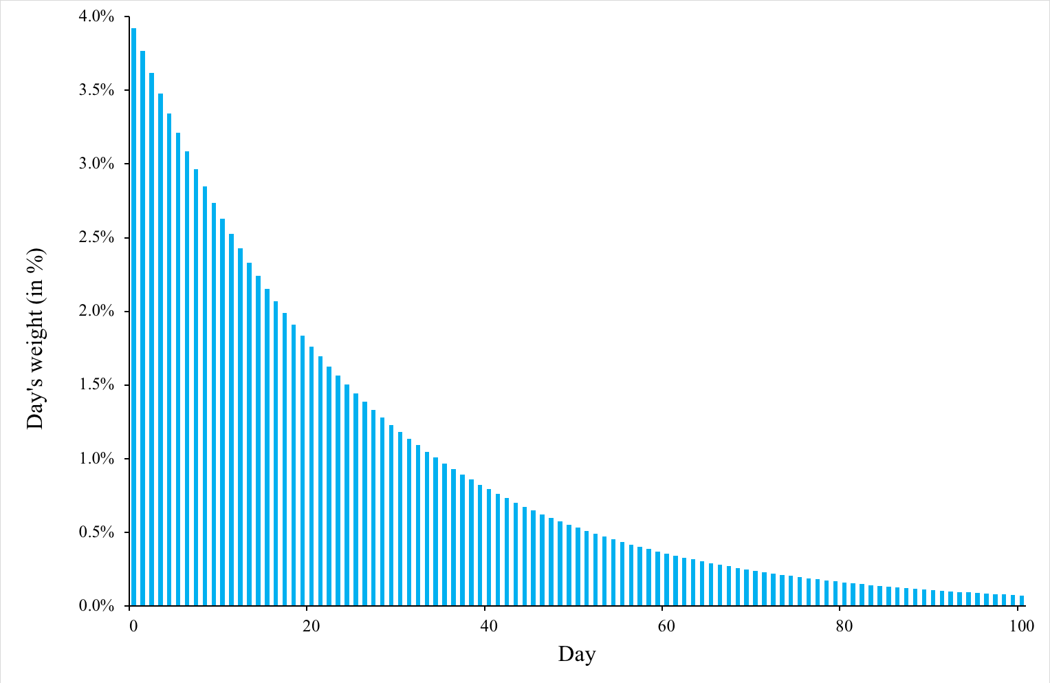
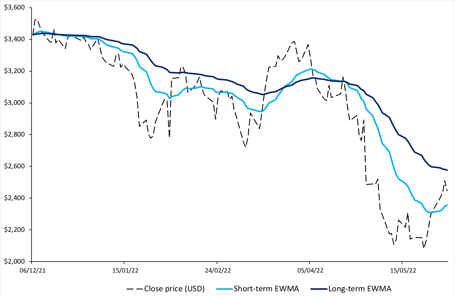
Market intelligence: I prepared real-time market reports and macro-driven trade ideas using Bloomberg. Bloomberg is a professional financial data platform used by banks, asset managers and corporates to monitor market prices, news, analytics and execution tools. My work involved following central-bank decisions, inflation data, interest-rate curves, energy markets and metals prices, then summarizing the implications for clients.
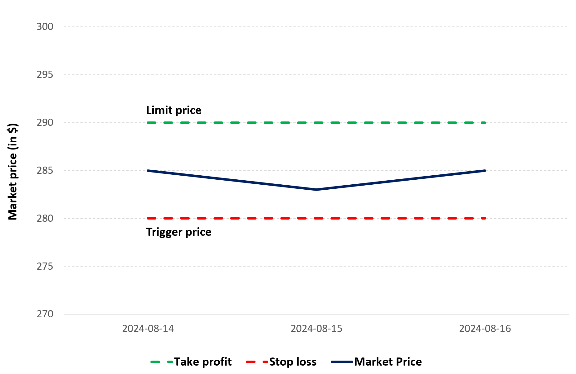
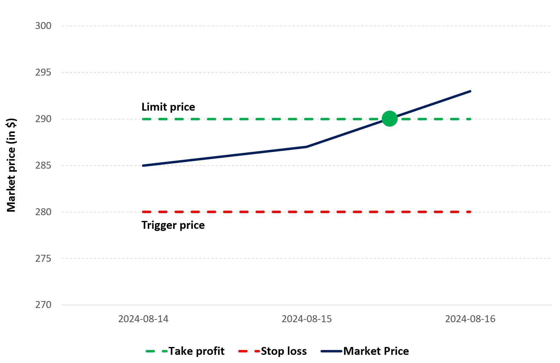
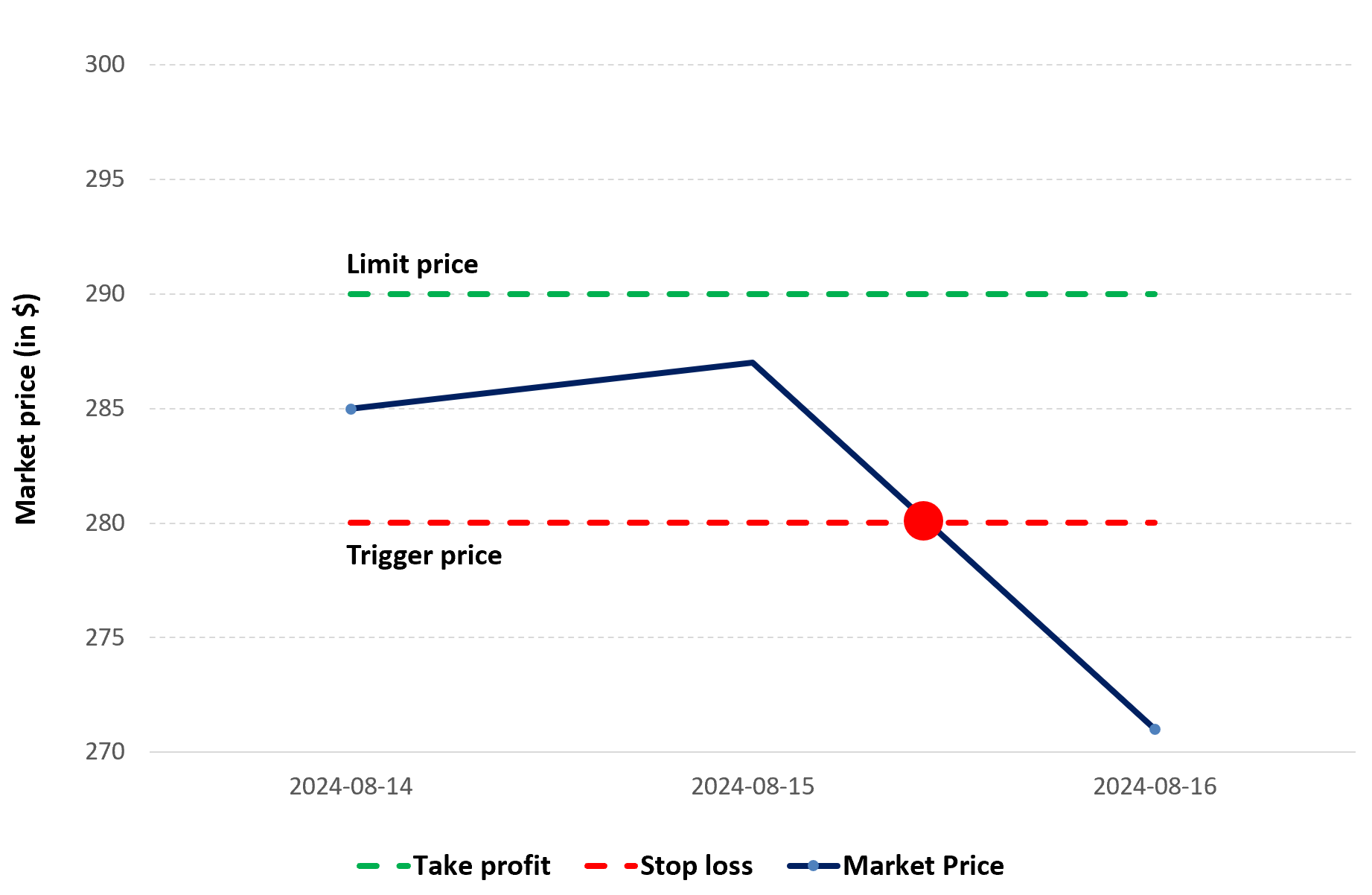
Product structuring: I worked on vanilla and semi-structured products such as forwards, swaps, options, collars and TARNs. A forward locks in a future price or exchange rate; a swap exchanges one stream of cash flows for another; an option gives protection or upside participation; a collar combines options to create a protection band; and a TARN (Target Redemption Note) is a structured product that terminates when a predefined target is reached.
Pricing and execution support: I worked day to day with traders to understand derivative pricing, bid-ask spreads and Greeks. The bid-ask spread is the difference between the price at which a dealer is willing to buy and the price at which it is willing to sell. The Greeks are risk measures used for options: for example, delta measures sensitivity to the underlying price, vega measures sensitivity to volatility and theta measures sensitivity to time decay.
Transaction process: I followed transactions from the client request to trade execution. This made me understand that the job requires both technical precision and process discipline: the client problem must be clearly identified, the structure must be suitable, the price must be executable and the documentation must be aligned with internal and regulatory requirements.
Commercial impact: From a core group of clients, the activity contributed approximately EUR 10k of daily revenues, primarily across oil & gas, energy and metals. This gave me a concrete view of how client relationships, market timing and product structuring can translate into measurable business results.
Required skills and knowledge
Hard skills: The internship requires knowledge of derivatives, fixed income, FX, commodities, option pricing, Bloomberg, macroeconomics, financial modeling and risk management. It also requires the ability to understand payoff profiles, compare hedging alternatives and interpret market data quickly.
Soft skills: The role also requires clear communication, attention to detail, speed under pressure and the ability to simplify complex market information. In derivatives sales, technical knowledge is useful only if it can be translated into a clear and relevant message for the client.
What I learned
The main lesson I learned is that derivatives sales is a bridge between markets and the real economy. A company does not hedge because a model says so; it hedges because volatility in oil, gas, metals, currencies or interest rates can directly affect its margins, debt service or investment plans.
I also learned that the quality of a trade idea depends on three elements: the market view, the client fit and the execution level. A correct macro view is not enough if the product is too complex for the client, too expensive to execute or misaligned with the company’s risk appetite.
Finally, the experience showed me the importance of discipline. Every price, spread, scenario and payoff profile must be checked carefully because derivatives can create both protection and risk. This is why sales and traders must work closely together before a transaction is executed.
Financial concepts related to my internship
I present below three financial concepts related to my internship experience:
Hedging with derivatives
Hedging means using financial instruments to reduce exposure to an unwanted risk. In my internship, typical risks include commodity price risk, FX risk and interest-rate risk. A commodity consumer may use swaps or options to stabilize future input costs; an exporter may use FX forwards to lock in an exchange rate; and a borrower may use interest-rate derivatives to reduce uncertainty around future financing costs.
Bid-ask spread and market making
The bid-ask spread is the difference between the price at which the bank can buy and the price at which it can sell a product. In derivatives, this spread compensates the bank for liquidity, hedging costs, market risk and operational complexity. Understanding the spread is important because it affects both the client’s execution level and the bank’s revenue.
Greeks and option risk management
The Greeks measure how the value of an option changes when market variables change. Delta measures sensitivity to the underlying price, gamma measures the change in delta, vega measures sensitivity to volatility, theta measures time decay and rho measures sensitivity to interest rates. These measures help traders hedge the risks created by client transactions and manage the desk’s exposure.
Why should I be interested in this post?
This post is relevant for ESSEC MiF students because it shows how financial theory becomes operational in a real banking environment. Courses on derivatives, portfolio management and financial markets provide the analytical foundation, but the internship shows how these tools are used under time pressure, with real clients and real market constraints.
For students interested in sales & trading, corporate banking or risk management, the role demonstrates that technical excellence and commercial understanding must go together. The best solutions are not necessarily the most complex ones, but the ones that are suitable, executable and useful for the client.
Related posts on the SimTrade blog
▶ All posts about Professional experiences
▶ Posts about derivatives and financial markets on the SimTrade blog
▶ Posts about trading and market making on the SimTrade blog
Useful resources
Banca Monte dei Paschi di Siena — Group website
Banca MPS — Commodity derivatives
Banca MPS — Foreign exchange derivatives
Banca MPS — Interest-rate derivatives
About the author
The article was written by Marco SIMONETTI (ESSEC Business School, MSc in Finance, 2025-2027), based on his experience as an Off-Cycle Sales & Trading Derivatives Intern at Banca Monte dei Paschi di Siena in Milan.
▶ Discover all articles by Marco SIMONETTI


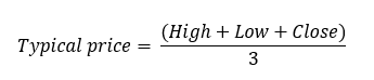


 Source: Computation by author.
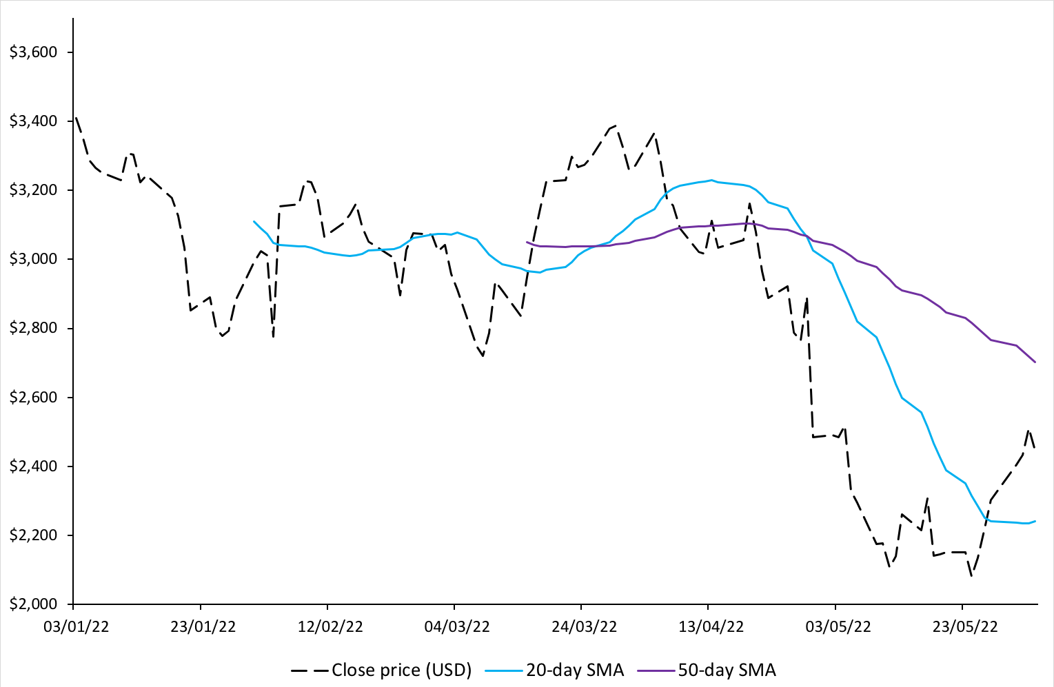