Black-Scholes-Merton option pricing model

In this article, Jayati WALIA (ESSEC Business School, Grande Ecole Program – Master in Management, 2019-2022) explains the Black-Scholes-Merton model to price options.

The Black-Scholes-Merton model (or the BSM model) is the world’s most popular option pricing model. Developed in the beginning of the 1970s, this model introduced to the world, a mathematical way of pricing options. Its success was essentially a starting point for new forms of financial derivatives in the knowledge that they could be priced accurately using the ideas and analyses pioneered by Black, Scholes and Merton and it set the foundation for the flourishing of modern quantitative finance. Myron Scholes and Robert Merton were awarded the Nobel Prize for their work on option pricing in 1997. Unfortunately, Fischer Black had died several years earlier but would certainly have been included in the prize had he been alive, and he was also listed as a contributor by Scholes and Merton.

Today, the Black-Scholes-Merton formula is widely used by traders in investment banks to price and hedge option contracts. Options are used by investors to hedge their portfolios to manage their risks.

Assumptions of the BSM Model

As any model, the BSM model relies on a set of assumptions:

• The model considers European options, which we can only be exercised at their expiration date.
• The price of the underlying asset follows a geometric Brownian motion (corresponding to log-normal distribution for the price at a given point in time).
• The risk-free rate remains constant over time until the expiration date.
• The volatility of the underlying asset price remains constant over time until the expiration date.
• There are no dividend payments on the underlying asset.
• There are no transaction costs on the underlying asset.
• There are no arbitrage opportunities.

The BSM equation

The value of an option is a function of the price of the underlying stock and its statistical behavior over the life of the option.

A commonly used model is Geometric Brownian Motion (GBM). GBM assumes that future asset price differences are uncorrelated over time and the probability distribution function of the future prices is a log-normal distribution (or equivalently the probability distribution function of the future returns is a normal distribution). The price movements in a GBM process can be expressed as:

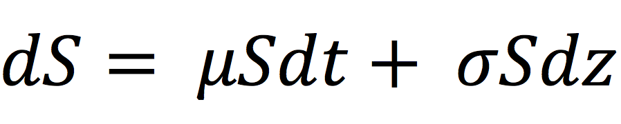
with dS being the change in the underlying asset price in continuous time dt and dX the random variable from the normal distribution (N(0, 1) or Wiener process). σ is the volatility of the underlying asset price (it is assumed to be constant). μdt represents the deterministic return within the time interval with μ representing the growth rate of asset price or the ‘drift’.

Therefore, option price is determined by these parameters that describe the process followed by the asset price over a period of time. The Black-Scholes-Merton equation governs the price evolution of European stock options in financial markets. It is a linear parabolic partial differential equation (PDE) and is expressed as:

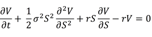
Where V is the value of the option (as a function of two variables: the price of the underlying asset S and time t), r is the risk-free interest rate (think of it as the interest rate which you would receive from a government debt or similar debt securities) and σ is the volatility of the log returns of the underlying security (say stocks).

The key idea behind the equation is to hedge the option and limit exposure to market risk posed by the asset. This is achieved by a strategy known as ‘delta hedging’ and it involves replicating the option through an equivalent portfolio with positions in the underlying asset and a risk-free asset in the right way so as to eliminate risk.

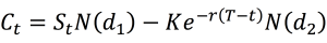
Thus, from the BSM equation we can derive the BSM formulae that describe the price of call and put options over their life time.

The BSM formulae

Note that the type of option we are valuing (call or put), the strike price and the maturity date do not appear in the above BSM equation. These elements only appear in the ‘final condition’ i.e., the option value at maturity, called the payoff function.

For a call option, the payoff C is given by:

C_T = max⁡(S_T – K; 0)

For a put option, the payoff is given by:

P_T = max⁡(K – S_T; 0)

The BSM formula is a solution to the BSM equation, given the boundary conditions (given by the payoff equations above). It calculates the price at time t for both a call and a put option.

The value for a call option at time t is given by:

The value for a put option at time t is given by:

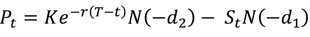
where

With the notations:
S_t: Price of the underlying asset at time t
t: Current date
T: Expiry date of the option
K: Strike price of the option
r: Risk-free interest rate
σ: Volatility (the standard deviation of the return on the underlying asset)
N(.): Cumulative distribution function for a normal (Gaussian) distribution. It is the probability that a random variable is less or equal to its input (i.e. d₁ and d₂) for a normal distribution. Thus, 0 ≤ N(.) ≤ 1

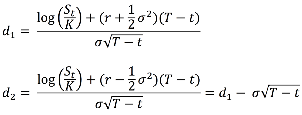
Figure 1 gives the graphical representation of the value of a call option at time t as a function of the price of the underlying asset at time t as given by the BSM formula. The strike price for the call option is 50€ with a maturity of 0.25 years and volatility of 50% in the underlying.

Figure 1. Call option value

Source: computation by author.

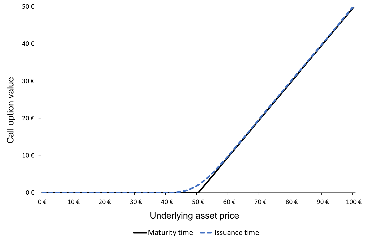
Figure 2 gives the graphical representation of the value of a put option at time t as a function of the price of the underlying asset at time t as given by the BSM formula. The strike price for the put option is 50€ with a maturity of 0.25 years and volatility of 50% in the underlying.

Figure 2. Put option value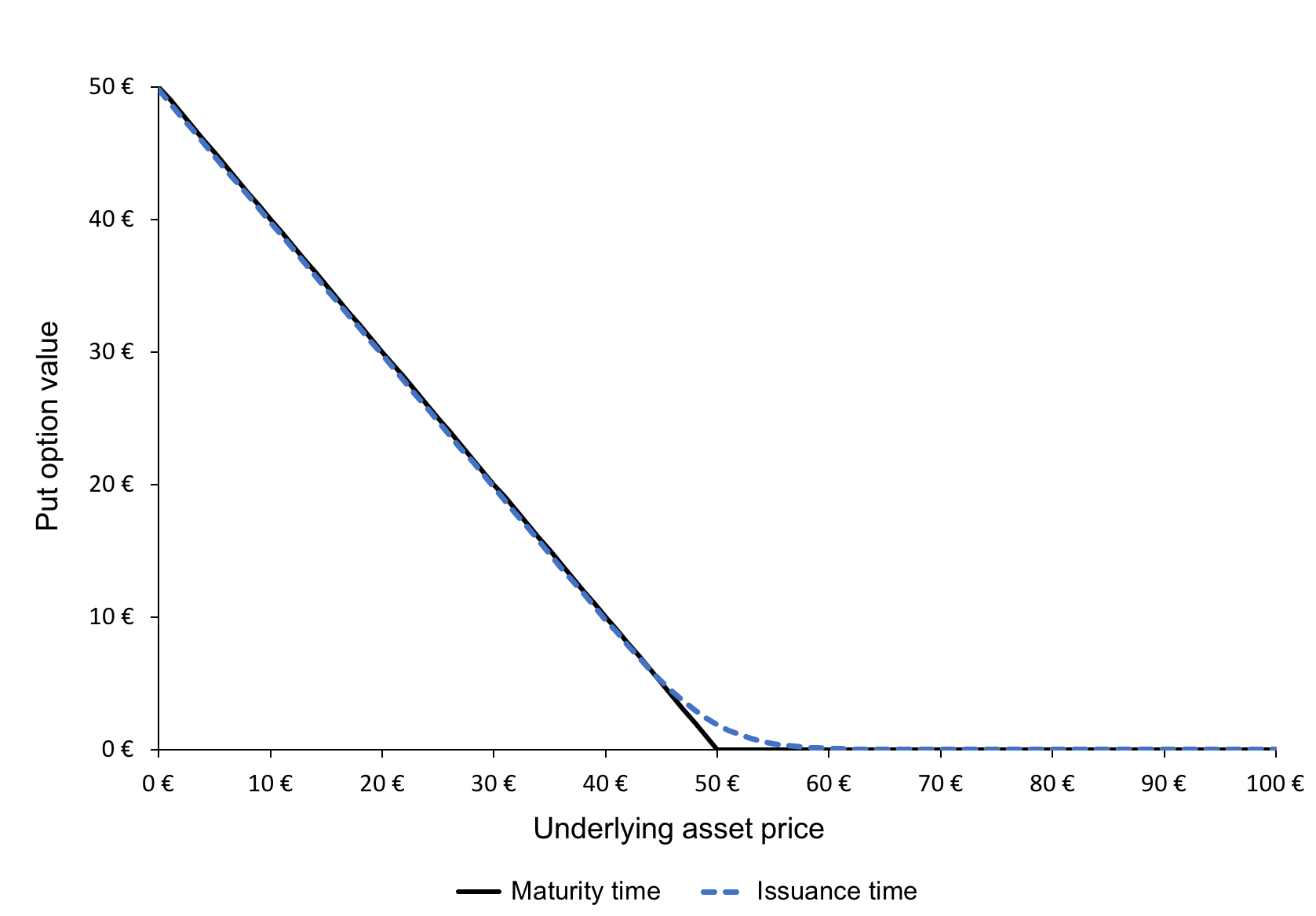
Source: computation by author.

You can download below the Excel file for option pricing with the BSM Model.

Some Criticisms and Limitations

American options

The Black-Scholes-Merton model was initially developed for European options. This is a limitation of the equation for American options which can be exercised at any time before the expiry date. The BSM model would then not accurately determine the option value (an important case when the underlying asset pays a discrete dividend).

Stocks paying dividends

Also, in reality, most stocks pay dividends, and no dividends was an assumption in the initial BSM model, which analysts now eliminated by accommodating the dividend yield in the formula if required.

Constant volatility

Another limitation is the use of constant volatility. Volatility is the measure of risk based on the standard deviation of the return on the underlying asset. In reality the value of an asset will change randomly, not with a specific constant pattern regarding the way it can change.

Finally, the assumption of no transaction cost neglects the liquidity risk in the market since transaction costs are clearly incurred in the real world and there exists a bid-offer spread on most underlying assets. For the most heavily traded stocks, this cost may be low but for others it may lead to an inaccuracy.

Related posts on the SimTrade blog

▶ All posts about Options

▶ Jayati WALIA Brownian Motion in Finance

▶ Akshit GUPTA Options

▶ Akshit GUPTA The Black-Scholes-Merton model

▶ Akshit GUPTA History of options market

Useful resources

Black F. and M. Scholes (1973) The Pricing of Options and Corporate Liabilities The Journal of Political Economy 81, 637-654.

Merton R.C. (1973) Theory of Rational Option Pricing Bell Journal of Economics 4, 141–183.

About the author

The article was written in March 2022 by Jayati WALIA (ESSEC Business School, Grande Ecole Program – Master in Management, 2019-2022).