How to download and model financial data with Python

Hadrien Puche

Any financial analysis starts with data. Whether you want to analyze a stock, build a portfolio, measure risk, create a valuation model or develop trading strategies, the first step is always the same: obtaining financial data.

You could download data manually from websites such as Yahoo! Finance or Investing.com, but this quickly becomes tedious and time-consuming. It also limits the amount of data you can work with.

Python allows us to automate this process and retrieve large amounts of financial information in just a few lines of code.

In this article, Hadrien Puche (ESSEC Business School, Grande École Program, Master in Management, 2023-2027) will help you understand how to:

  • Download historical stock prices with Python
  • Explore and visualize market data
  • Compute basic statistics and historical distributions
  • Compare multiple securities
  • Learn more about the CAPM
  • Build the foundation needed for more advanced financial analysis

What financial data can we download?

Financial professionals use many different categories of data across individual assets as well as portfolios and funds.

Market data

  • Individual asset prices (e.g., individual stocks, corporate bonds)
  • Portfolios and funds (e.g., ETFs, mutual funds)
  • Currency exchange rates
  • Commodity prices
  • Bond yields

Company fundamentals

  • Revenue
  • Earnings
  • Margins
  • Cash flows

Macroeconomic data

  • Inflation
  • Interest rates
  • GDP growth
  • Unemployment

Alternative data

  • News
  • Social media sentiment
  • Satellite imagery
  • Credit card spending

Not all data sources are freely available. Many professional investors rely on paid platforms such as Bloomberg, FactSet, Capital IQ or Morningstar to access standardized, high-frequency, and point-in-time data.

Fortunately, stock market data specifically can easily be accessed for free using Python for research and learning purposes.

In this article, we will use the open-source yfinance library to download historical market data that you will then be able to model and use for any financial analysis project you may have.

A step-by-step guide

Follow the next steps to download your first financial data with Python 🙂

Step 1: Installing the required libraries

If you have not yet installed Python, refer to the setup guide to configure your execution environment (such as Jupyter Notebook or Anaconda).

Once your environment is ready, install the required packages:

pip install yfinance pandas numpy matplotlib

or inside Jupyter Notebook:

!pip install yfinance pandas numpy matplotlib

We will use:

  • yfinance to retrieve market data
  • pandas to manipulate data structures
  • numpy for financial and mathematical operations
  • matplotlib to create charts

Step 2: Import our Python packages

Most data analysis scripts begin by importing the packages required for the analysis. In Python, packages provide reusable code and functionality that extend Python’s core capabilities.

import yfinance as yf
import pandas as pd
import numpy as np
import matplotlib.pyplot as plt

The aliases (yf, pd, np, plt) make the code shorter and easier to read.

Step 3: Download our first data set

To download financial data, we use ticker symbols, which identify securities or market instruments within a given exchange or data provider. For example, AAPL represents Apple.

When calling a Python function, we can customize its behavior by passing arguments such as period (e.g., "5y" for 5 years) or specific start and end dates.

As an example, let us download daily data for Apple stock price over the last five years (Yahoo! Finance ticker: AAPL). The data will be stored in a data frame (df) that we can name df_apple.

df_aapl = yf.download("AAPL", period="5y")

print(df_aapl.head())

You will obtain this table with the following columns:

  • Close: closing price at the end of the trading day
  • High: highest price during the trading day
  • Low: lowest price during the trading day
  • Open: opening price at the beginning of the trading day
  • Volume: transaction volume during the trading day
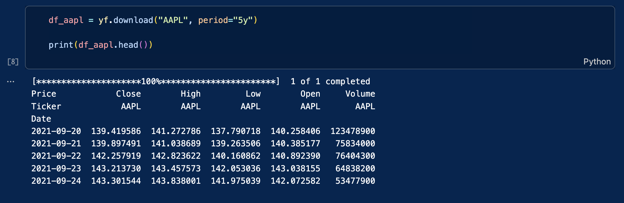
An screenshot from VSC showing the output table of this Yfinance query

The data is stored in a Pandas DataFrame. This is a popular two-dimensional, tabular data structure with labeled axes (rows and columns).

To inspect its structure, type the following code:

df_aapl.info()
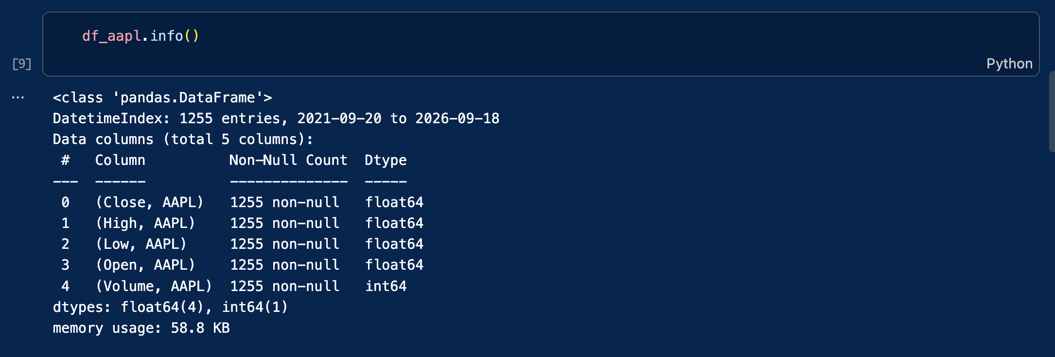
A screenshot from VSC showing the output of df_aapl.info()

Step 4: Using more precise queries for historical context

Instead of downloading a rolling period (like “5y”), we can isolate specific market events by passing exact start and end dates to the download function. As financial analysts, we routinely extract specific timeframes to understand how assets behave under macroeconomic stress.

For example, analyzing the COVID-19 market crash in early 2020 offers invaluable insights into extreme volatility, liquidity crunches, and rapid V-shaped recoveries. Let’s download and plot Apple’s stock specifically during the height of the pandemic shock (January to June 2020):

# Isolate the COVID-19 crash and initial recovery phase
covid_crash = yf.download("AAPL", start="2020-01-01", end="2020-06-30")

# Plot the isolated data
plt.figure(figsize=(10, 5))
plt.plot(covid_crash.index, covid_crash["Close"], color="#d9534f", linewidth=2)
plt.title("AAPL Stock Price - COVID-19 Crash & Recovery (Early 2020)")
plt.xlabel("Date")
plt.ylabel("Price ($)")
plt.grid(True, linestyle="--", alpha=0.6)
plt.show()
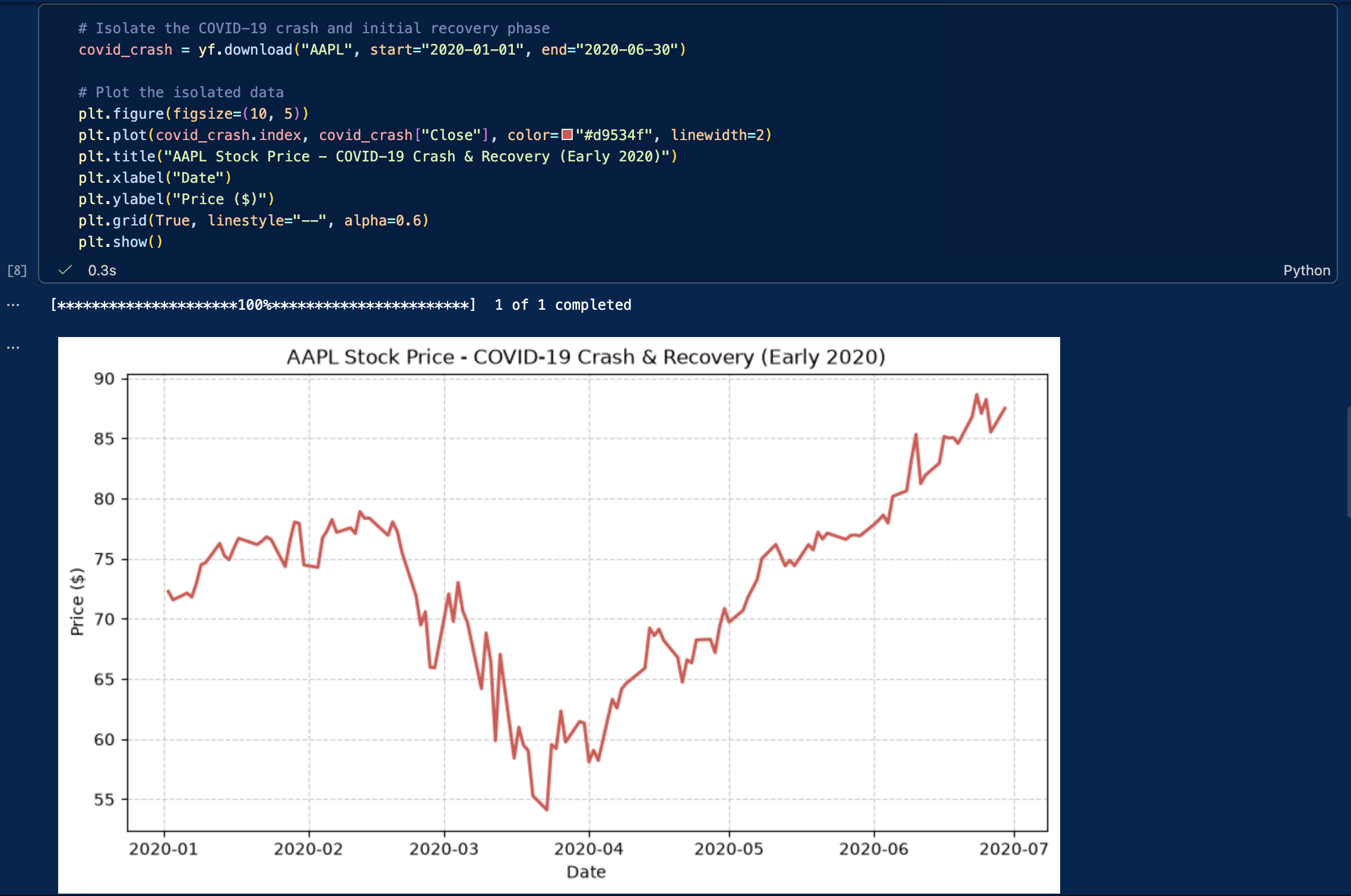
The output of the previous code cell

We could use this same technique to analyze other pivotal periods, such as:

  • A central bank interest rate tightening cycle (e.g., the Fed’s 2022-2023 rate hikes)
  • The 2008 Global Financial Crisis (if analyzing older datasets)
  • Specific earnings announcement windows

Step 5: Downloading multiple stocks at the same time

Downloading multiple stocks is necessary for financial analysis that often requires comparing securities, building a portfolio, or testing trading strategies like pairs trading.

Instead of issuing separate requests for each stock (which risks hitting API rate limits or misaligning dates), it is far more efficient to fetch all tickers at once in a single batch query.

To make this practical, let’s download the data for the “Magnificent Seven”. These seven mega-cap tech companies (Apple, Microsoft, Alphabet, Amazon, Meta, Nvidia, and Tesla) have heavily dominated market capitalization and driven a massive portion of the S&P 500’s returns in recent years.

# Define the Magnificent 7 tickers
mag7_tickers = ["AAPL", "MSFT", "GOOGL", "AMZN", "META", "NVDA", "TSLA"]

# Download the closing prices for all 7 stocks simultaneously
prices = yf.download(mag7_tickers, period="5y")["Close"]
 
print(prices.head())

The result is now again a matrix where each column represents a stock, and each row represents a trading day.
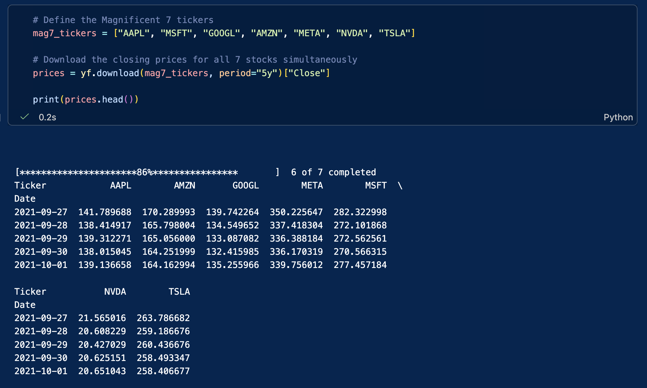
Screenshot of the output of the previous cell

This table format is ideal for portfolio analysis, benchmarking, and performance comparisons, and can be used to draw any kind of graphs.

Note that the table’s columns are displayed in two groups. Depending on the display width, Jupyter Notebook or VS Code may wrap or truncate wide DataFrames. You can export the DataFrame to a CSV file if you prefer to inspect the complete dataset in a spreadsheet application.

# save the dataframe as a csv
prices.to_csv('mag_7_data.csv')
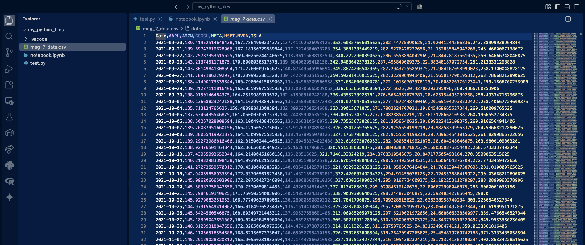
Screenshot of the output of the previous cell

Now that you successfully downloaded your financial data, let’s see how you can clean it and then use it.

Inspecting and cleaning the dataset

Financial datasets may contain missing values (NaN) for various reasons, including differences in trading calendars, trading suspensions, listing dates, or data-provider issues. Missing observations should be identified before computing returns or risk measures. For this introductory example, we simply remove rows containing missing values. In applied financial analysis, however, the appropriate treatment depends on the source of the missing data and the objective of the analysis.

If left unaddressed, these missing data points will break your mathematical functions and severely distort your return and volatility calculations. The code below checks how many missing values exist in each column, and then removes (drops) any rows containing them. In some situations you might want to forward-fill these gaps to preserve the timeline, but dropping them is the safest thing to do for now.

# Check for missing values
print(df_aapl.isnull().sum())
# Clean missing values by dropping rows with NaNs
df_aapl = df_aapl.dropna()
# Print the first rows of the dataframe
df_aapl.head()
df_aapl.head()
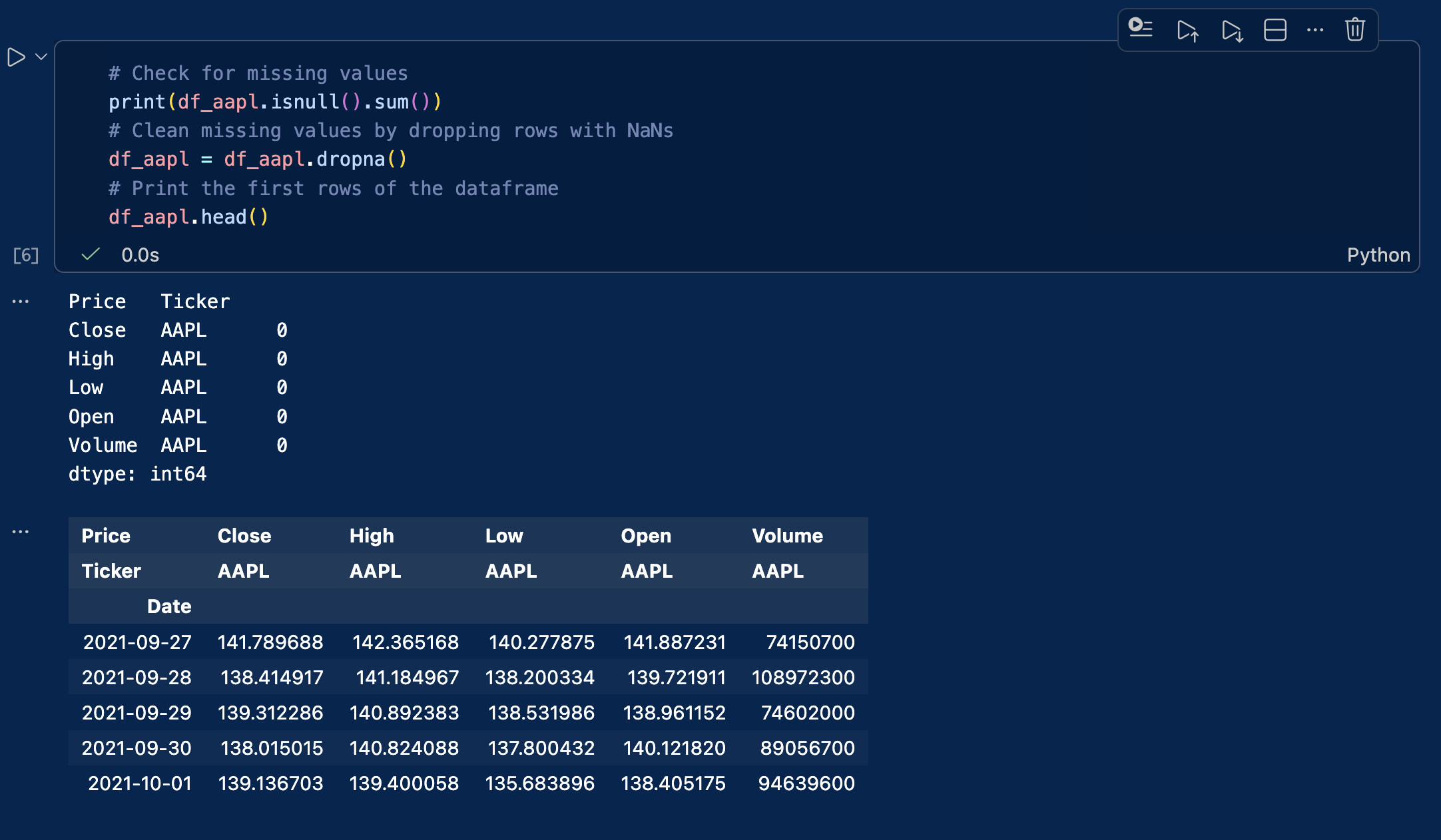
A screenshot from VSC showing the output of the cleaning code cell

To view the last rows of the dataframe, replace head() by tail():
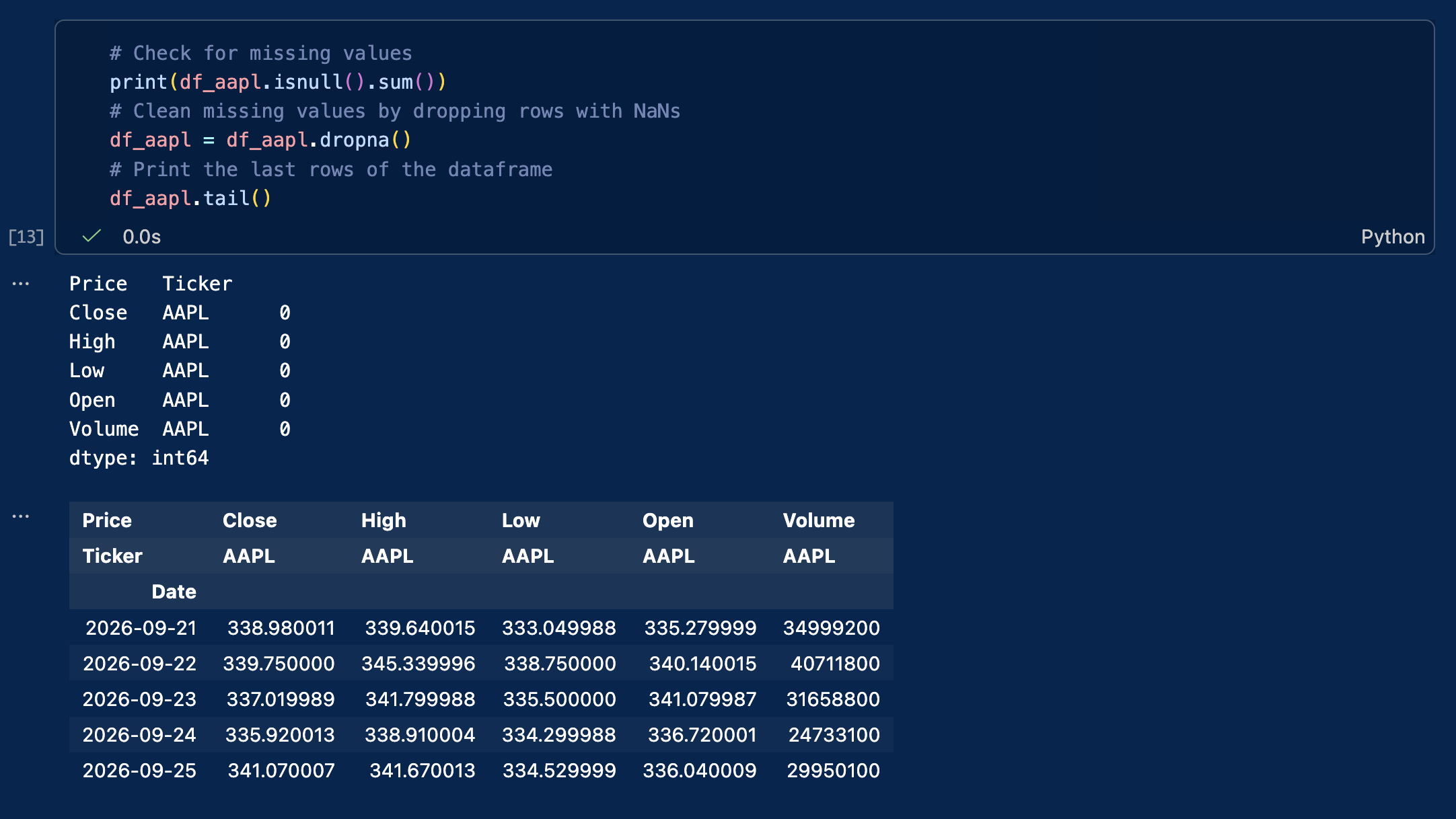
Output of the VSC cell when we switch to tail()

Visualizing the stock price with graphs or charts

Let’s create our first graph to visualize the evolution of Apple’s stock price.

plt.figure(figsize=(10, 5))
plt.plot(df_aapl.index, df_aapl["Close"], label="AAPL Close Price")
plt.title("Apple Stock Price")
plt.xlabel("Date")
plt.ylabel("Price ($)")
plt.legend()
plt.show()
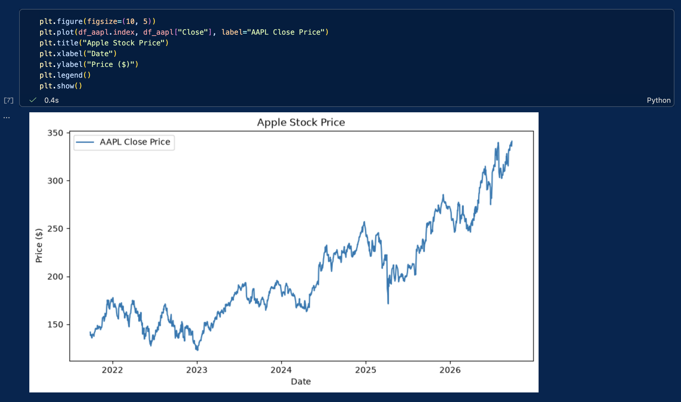
A screenshot of VSC with the stock price visualization cell output

We have now:

  • Downloaded market data from Yahoo! Finance
  • Stored and cleaned the data in a dataframe
  • Created a time-series plot to visualize stock prices

These core steps form the basis of empirical financial research and quantitative models.

Computing basic statistics & historical distributions

To evaluate stock performance and risk, we compute basic descriptive statistics for both prices and financial returns: minimum, maximum, mean, variance, standard deviation, skewness, and kurtosis. Although descriptive statistics can also be computed for price levels, risk analysis generally focuses on returns, whose distributions are more economically meaningful.

# Calculate daily percentage returns
df_aapl['Return'] = df_aapl['Close'].pct_change()

# Compute summary statistics for Price and Returns
stats_df = pd.DataFrame({
    'Metric': ['Min', 'Max', 'Mean', 'Variance', 'Std Dev', 'Skewness', 'Kurtosis'],
    'Price ($)': [
        df_aapl['Close'].min().item(),
        df_aapl['Close'].max().item(),
        df_aapl['Close'].mean().item(),
        df_aapl['Close'].var().item(),
        df_aapl['Close'].std().item(),
        df_aapl['Close'].skew().item(),
        df_aapl['Close'].kurtosis().item()
    ],
    'Daily Return': [
        df_aapl['Return'].min().item(),
        df_aapl['Return'].max().item(),
        df_aapl['Return'].mean().item(),
        df_aapl['Return'].var().item(),
        df_aapl['Return'].std().item(),
        df_aapl['Return'].skew().item(),
        df_aapl['Return'].kurtosis().item()
    ]
})

print(stats_df)

Plotting historical distributions

Histograms display the frequency distribution of prices and daily returns, helping us inspect price trends, distribution symmetry, and tail risks.

fig, axes = plt.subplots(1, 2, figsize=(14, 5))

# Price distribution
axes[0].hist(df_aapl['Close'].dropna(), bins=30, color='skyblue', edgecolor='black')
axes[0].set_title('Historical Price Distribution')
axes[0].set_xlabel('Price ($)')
axes[0].set_ylabel('Frequency')

# Return distribution
axes[1].hist(df_aapl['Return'].dropna(), bins=50, color='salmon', edgecolor='black')
axes[1].set_title('Historical Daily Return Distribution')
axes[1].set_xlabel('Daily Return')
axes[1].set_ylabel('Frequency')

plt.tight_layout()
plt.show()

Normalizing stock prices and computing returns

All stocks have different nominal prices. If Tesla trades at $350 and Nvidia at $220, it does not mean that Tesla is worth more than Nvidia or performed better.

To establish an accurate comparison across these assets, we must execute two fundamental computations:

  1. Price harmonization: we normalize all historical time series to a base index of 100, to ensure a standardized starting point.
  2. Return calculation: we compute the periodic returns to get the actual performance in % rather than the absolute variation.
normalized = prices / prices.iloc[0] * 100

plt.figure(figsize=(10, 5))
plt.plot(normalized.index, normalized)
plt.title("Performance Comparison (Base = 100)")
plt.xlabel("Date")
plt.ylabel("Growth of $100")
plt.legend(prices.columns)
plt.show()
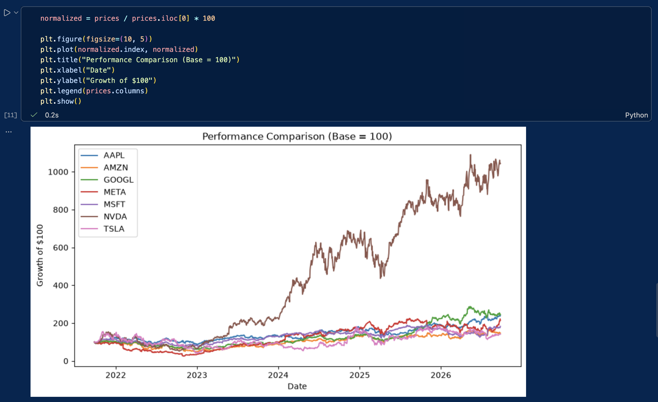
the output of the previous cell

We can also compute daily returns across all stocks:

returns = prices.pct_change().dropna()
print(returns.head())
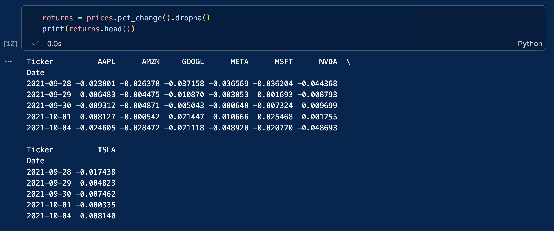
the output of the previous cell

The chart now shows how much each investment would have grown from the same starting value.

This is a standard technique used by portfolio managers and equity analysts.

Case study: the Capital Asset Pricing Model (CAPM)

In empirical finance, evaluating an individual asset requires isolating the return generated by the broader market from the return specific to the company itself. The Capital Asset Pricing Model (CAPM) provides the foundational framework to decompose this risk.

The model decomposes the return of an individual asset over a given time period into three components: the risk-free rate, a market systematic factor and a firm-specific factor. The model is expressed through the following equation:

rt = rf + β(rm – rf) + εt

Where:

  • rt is the return of the stock (e.g., Apple).
  • rf is the risk-free interest rate (e.g., the 13-week Treasury Bill, ^IRX).
  • β (Beta) represents the stock’s sensitivity to market movements (systematic risk).
  • rm – rf is the excess return of the market index (e.g., the S&P 500, ^GSPC).
  • εt (Epsilon) represents the idiosyncratic return associated with firm-specific risk not explained by the market.

By downloading these three time series simultaneously, we can calculate the stock’s Beta and isolate its firm-specific residual risk.

# Download asset (AAPL), market benchmark (S&P 500), and risk-free rate (13-week T-Bill)
market_data = yf.download(["AAPL", "^GSPC", "^IRX"], start="2022-01-01", end="2024-12-31")["Close"].dropna()

# Compute daily percentage returns for the stock and the market
returns_df = market_data[["AAPL", "^GSPC"]].pct_change().dropna()
 
# Convert the annualized risk-free yield (^IRX) to a daily rate
daily_rf = (market_data["^IRX"] / 100) / 252
returns_df["Rf"] = daily_rf
 
# Calculate the excess returns: (r_t - r_f) and (r_m - r_f)
excess_aapl = returns_df["AAPL"] - returns_df["Rf"]
excess_market = returns_df["^GSPC"] - returns_df["Rf"]
 
# Compute Market Beta: Covariance(stock, market) / Variance(market)
cov_matrix = np.cov(excess_aapl, excess_market)
beta = cov_matrix[0, 1] / cov_matrix[1, 1]
 
# Isolate Epsilon (the firm-specific residual risk)
# Rearranging the CAPM equation: epsilon = (r_t - r_f) - beta * (r_m - r_f)
epsilon = excess_aapl - (beta * excess_market)
 
print(f"Calculated Beta: {beta:.4f}")
print(f"Mean Firm-Specific Return (Epsilon): {epsilon.mean():.6f}")
print(f"Idiosyncratic Risk (Epsilon Std Dev): {epsilon.std():.4f}")

Common pitfalls

When working with market data, beginners often run into the same issues:

  • Using the wrong ticker symbol
  • Comparing stocks without normalizing prices
  • Forgetting that markets are closed on weekends and holidays
  • Failing to clean and handle missing values (NaN) in the dataset
  • Failing to check whether price series are raw or adjusted for stock splits and dividends

Overall, always inspect and clean your data before starting your analysis.

Exercises

Exercise 1: Basic data retrieval and price visualization (MSFT)

Microsoft is a mature mega-cap technology company, and a cornerstone of most global equity portfolios. Retrieving and inspecting its historical data is a perfect starting point to practice basic YFinance commands.

Using the ticker symbol MSFT, download the last five years of daily market data.

Your tasks:

  • Use the appropriate pandas functions to display the first 5 rows and the last 5 rows of the dataset to verify data integrity (checking for correct start/end dates).
  • Generate a line chart plotting the closing price over the entire 5-year period to visualize its long-term market trend.

Exercise 2: time-series extraction and volume analysis on Tesla (TSLA)

Tesla is renowned for its high historical volatility and massive retail trading interest. The 2022-2024 window was particularly eventful for growth and electric vehicle stocks, marked by shifting supply chains and a rapid rise in interest rates. Isolating this exact timeframe allows us to analyze the stock’s behavior under changing macroeconomic conditions.

Using the ticker symbol TSLA, extract the market data for the precise calendar period from January 1, 2022, to December 31, 2024 (using the start and end parameters).

Your tasks:

  • Identify the peak (highest closing price) and the trough (lowest closing price) over this period to grasp the magnitude of the stock’s price swings.
  • Calculate the average daily trading volume, a fundamental metric used by analysts to assess market liquidity and ongoing investor interest.

Exercise 3: Comparative performance and risk profiling on Chinese tech companies

Chinese technology stocks often experience unique market cycles driven by distinct domestic regulatory environments and macroeconomic factors. Using their US-listed ADRs (American Depositary Receipts), compare the performance and risk characteristics of three major players over the last five years:

  • Alibaba (BABA)
  • Baidu (BIDU)
  • PDD Holdings (PDD)

Questions:

  1. Which stock achieved the highest total cumulative return?
  2. Which stock was most volatile (highest standard deviation of daily returns)?
  3. Which one offered the best risk-adjusted profile (e.g., highest Sharpe ratio) over the period?

Download the solutions

To help you check your work and experiment further, you can download the complete Jupyter Notebook containing the full code, charts, and commentary for all exercises.

Download Solutions (.ipynb)

Once downloaded, change the file’s extension from .txt to .ipynb and open it in Visual Studio code.

What’s next?

Now that you know how to download financial data, perform basic computations, and control for market risk, you are ready to delve into advanced quantitative and corporate finance topics.

About the author

This article was written in September 2026 by Hadrien PUCHE (ESSEC Business School, Grande École Program, Master in Management, 2023-2027).

   ▶ Discover all posts by Hadrien PUCHE
How to Install and Run Python on Your Computer (A Step-by-Step Guide)

Hadrien Puche

In finance, the ability to rapidly acquire, clean, and manipulate data is a key skill that can help you gain an edge over other students and job applicants. While Excel (with VBA) remains widely used and is sufficient for most basic financial modeling, such as a DCF valuation, Python offers far more scalability, automation, and mathematical power than Excel.

In this article, Hadrien PUCHE (ESSEC Business School, Grande École Program, Master in Management, 2023-2027) will help you to:

  • Understand the core components of a Python environment for finance
  • Choose the most secure and efficient development setup for financial data
  • Install Miniconda and manage isolated virtual environments
  • Set up Visual Studio Code (VS Code) as your primary coding workspace
  • Run a test script to download and visualize real stock market data

No computer science background is required to start using Python.

Quick vocabulary for beginners

Before we dive in, let’s demystify a few technical terms you will encounter frequently:

  • Python: A popular, high-level programming language created in 1991 by Guido van Rossum (and named after the BBC comedy series Monty Python’s Flying Circus). Today, Python is widely used in quantitative finance and data science because of its simple syntax and vast ecosystem of financial tools.
  • Library / Package: A collection of pre-written code created by other developers so you don’t have to reinvent the wheel (e.g., pandas for data tables, yfinance for downloading stock market prices).
  • Dependency: A package that another package needs in order to work properly.
  • Environment: An isolated “sandbox” on your computer containing a specific version of Python and specific libraries, preventing projects from interfering with one another.
  • IDE (Integrated Development Environment): The visual software app where you write, edit, and test your code (e.g., Visual Studio Code).
  • Extension: An add-on (like an app from an App Store) that adds extra features to your IDE.

In this first article, we will focus on helping you set up Python on your computer so that you can start learning how to use it. We will guide you step by step through setting up a professional local workspace and testing that everything is working properly. Once that is done, you will find a list of follow-up articles at the end to explore real-world financial use cases.

Choosing your development environment

A development environment is simply the ecosystem of software tools you use to write, manage, and execute your code. When selecting a workspace for Python, you have three main choices:

  • Local workspaces (like Visual Studio Code): The standard choice for finance. Running your code locally (on your own computer) gives you full control over your local file systems, execution speed, and (most importantly) data privacy. In finance, working with proprietary trading algorithms or confidential client data means you cannot upload sensitive information to unvetted third-party servers.
  • Cloud notebooks (like Google Colab): Cloud platforms are convenient for quick experiments because they require zero installation. However, they are generally unsuitable for professional financial workflows. You do not have full control over code execution or environment stability, and uploading confidential financial datasets or proprietary logic to public cloud infrastructure poses significant security and compliance risks.
  • AI-native code editors (like Cursor or Windsurf): These editors heavily integrate AI to generate code automatically. While powerful for experienced developers, relying on AI tools too early prevents beginners from learning core programming logic, syntax, and debugging skills. It is far better to understand the core mechanics manually first.

In this article, we will focus exclusively on establishing a local workspace using Visual Studio Code (VS Code),which is a widely used tool to get comfortable with professional Python coding.

We will also use Jupyter Notebooks (files ending in .ipynb). Unlike traditional Python scripts (files ending in .py) that execute the entire code at once, Jupyter Notebooks allow you to write and run code in individual “cells.” This block-by-block structure is especially powerful in finance for several reasons:

  • Isolating code: You can work on and execute specific parts of your code independently (e.g., downloading data once, then tweaking the math in a separate cell without re-downloading).
  • Immediate feedback: Data tables, charts, and outputs are displayed directly below the specific cell you just ran, and you do not have to execute the entire code each time.
  • Easier debugging: By testing your logic piece-by-piece, identifying and fixing errors becomes significantly faster.
  • Better examples, tutorials, or exercises: You can mix executable code with explanatory text and financial formulas, making it the perfect format for case studies and tutorials.

As your code grows, using a Jupyter Notebook will be more and more useful.

What you need to install (and why)

Before installing anything, let’s understand how the different components of your workspace fit together:

  • Miniconda (which includes Python & Conda): Python comes with a comprehensive standard library, but financial and data analysis typically require additional packages such as pandas, NumPy, matplotlib, and yfinance. To perform financial analysis, you need external packages/libraries like pandas or yfinance. Conda is a tool that manages these packages and isolates them into dedicated virtual environments.
    Note on Anaconda vs. Miniconda: Anaconda is a big download that comes bundled with hundreds of packages you may never use. I suggest using Miniconda because it is a lightweight version, containing only Conda and Python, allowing us to keep your setup clean and fast.
  • Virtual Environments: Why do we need them? If you install every package into one single base Python installation, different projects will eventually require conflicting versions of the same library (a “dependency collision”), causing your scripts to crash. Virtual environments keep each project’s tools safely separated.
  • Visual Studio Code (VS Code): A clean user interface where you write, edit, and debug your code. VS Code connects seamlessly to your Conda virtual environment to execute your scripts.

How the architecture works

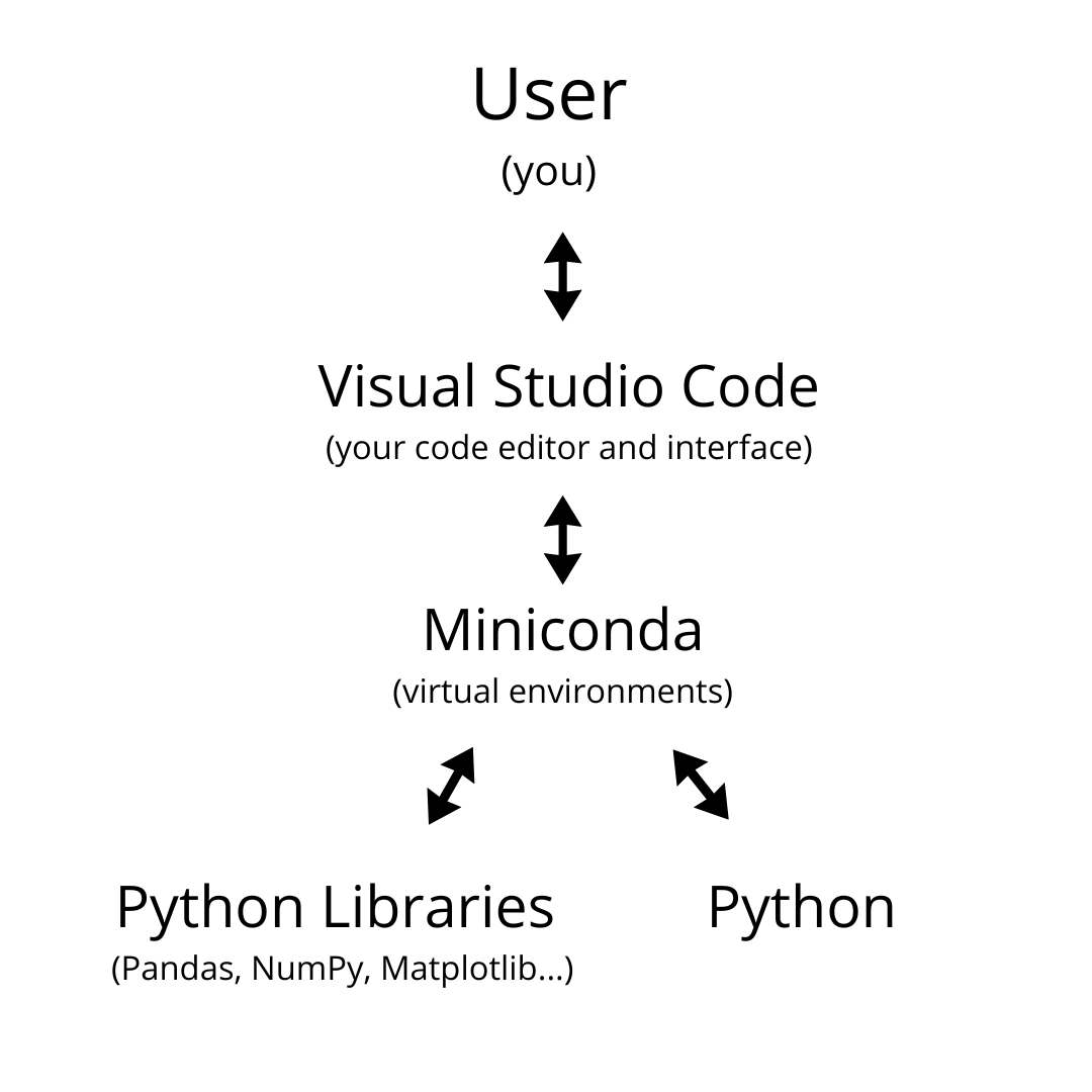
The diagram below illustrates how your development setup functions:

A graph showing the links between the user, VS Code, Miniconda, and Python.
Figure 1: How the User, VS Code, Miniconda Environment, and Python Engine interact.

  • You (the User) interact directly with VS Code to write commands and inspect results.
  • VS Code sends your code to your isolated Miniconda Virtual Environment (e.g., my_environment that you can create to store the packages that you will use in your own code).
  • Inside this environment, the Python Engine processes the math and logic, drawing upon the installed financial libraries (like yfinance and pandas).
  • The execution results (tables, charts, output logs) are sent back to VS Code for you to view.

As a fun side note: you can technically write code in almost any text editor! For a fun take on how far you could take this, check out this video.

Step-by-step installation guide

Step 1: Install Miniconda (Python + Conda)

Conveniently, downloading and installing Miniconda automatically installs Python, so this will be our first step.

Head to the official Miniconda Download Page, select the installer for your operating system (Windows or macOS), and complete the installation using the recommended default settings.

Step 2: Install Visual Studio Code and Extensions

Visual Studio Code (VS Code) will serve as your Integrated Development Environment (IDE). As a quick reminder, an IDE is the main visual software application, where you will actually write, edit, test, and debug your code. You can think of it as the central command dashboard for all your financial programming projects.

  1. Download & Install: Go to the official VS Code website, download the installer for Windows or macOS, and follow the standard installation instructions.
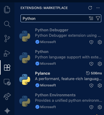
  2. Install Essential Extensions: Launch VS Code. Click on the Extensions icon on the left-hand Activity Bar (or press Ctrl+Shift+X on Windows / Cmd+Shift+X on Mac). Think of extensions as add-ons from an app store that give VS Code superpowers. Search for and install:
    • Python (by Microsoft) – Provides syntax highlighting, code completion, and interpreter selection.
    • Jupyter (by Microsoft) – Enables interactive execution of code cells inside .ipynb notebook files.

VS Code Extensions Marketplace showing Python extension by Microsoft
Make sure to install the official Python and Jupyter extensions in VS Code.

Step 3: Create your virtual environment via the Terminal

Now, we will create a clean, isolated Conda environment named my_environment where our financial packages will live.

  1. Open your command line interface:
    • Windows 11 / 10: Open the Start menu, search for Anaconda Prompt, and click to open it. (Alternatively, you can open Windows Terminal / PowerShell, but Anaconda Prompt automatically initializes Conda for you).
    • macOS: Open the Terminal app (press Cmd + Space, type “Terminal”, and press Enter).
  2. Run the following Conda & pip commands one by one:
# 1. Create an isolated environment named ‘my_environment’ with Python 3.11 conda create –name my_environment python=3.11 -y # 2. Activate your new environment conda activate my_environment # 3. Upgrade pip and install core financial analysis libraries pip install –upgrade yfinance pandas numpy matplotlib notebook –no-cache-dir

Pro-tip: Whenever you need to install additional packages in the future, open your terminal, activate your environment (conda activate my_environment), and run pip install [package_name].

Step 4: Connect VS Code to your environment

Now that your environment and libraries are ready, you need to tell VS Code to use my_environment to run your code.

  1. Open a workspace folder: In VS Code, go to File > Open Folder… and select or create a dedicated folder on your computer (e.g., finance_python). It does not matter where it is, you simply need somewhere to store your code files.
  2. Create your files: Click the New File icon in the Explorer sidebar to create two files:
    • test.py (.py file is to store Python code)
    • notebook.ipynb (.ipynb is the file extension name used for Jupyter notebooks)
  3. Select the Python interpreter: Open test.py. Press Ctrl+Shift+P (Windows) or Cmd+Shift+P (macOS) to open the Command Palette, type Python: Select Interpreter, and press Enter.
    • VS Code should automatically list my_environment. Click on it.
    • If it doesn’t appear automatically: Click Enter interpreter path… > Find… and navigate directly to the executable file:
      • Windows: C:\Users\YourUsername\miniconda3\envs\my_environment\python.exe
      • macOS: /Users/YourUsername/miniconda3/envs/my_environment/bin/python3
  4. Select Jupyter Kernel: Open notebook.ipynb. Click Select Kernel in the top-right corner of the window, choose Python Environments…, and select your my_environment path.

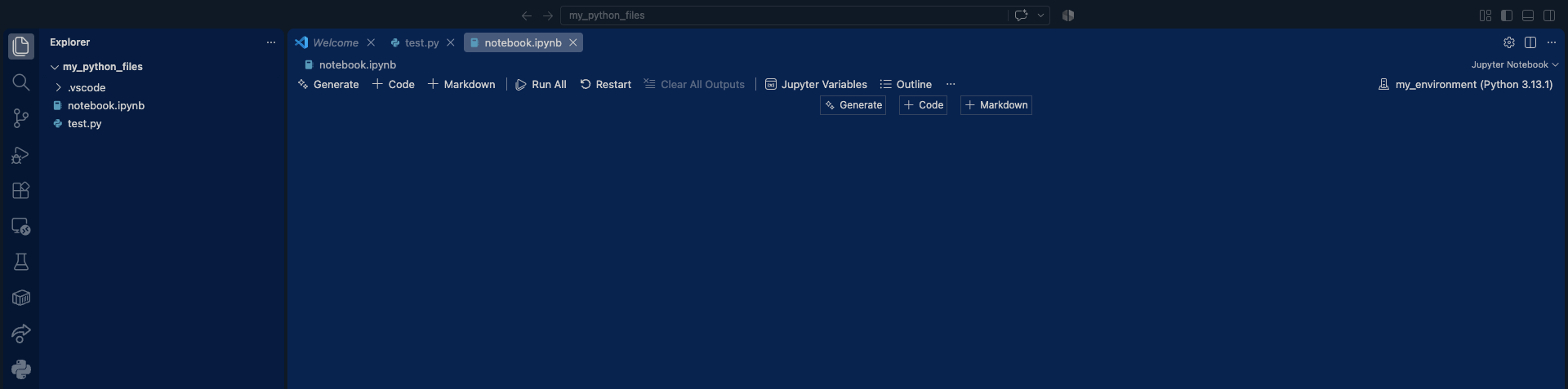
An image of the VS Code menu with notebook.ipynb and test.py created
Once this is done, your IDE should look just like this.

Quick Troubleshooting Tips:
  • “No matching commands” error: If typing Python: Select Interpreter gives no results, click inside the test.py editor window first to wake up the Python extension, or click Select Python Interpreter in the bottom-right status bar.
  • Environment missing from the list: Make sure you activated the environment in terminal at least once, or use the direct path navigation detailed above.

Testing your installation

Now that VS Code is connected to my_environment, let’s run a simple test script to confirm that our setup can successfully fetch market data and display a stock chart. Open test.py or notebook.ipynb, paste the code below, and execute it:

# Import yfinance to download stock market data directly from Yahoo Finance
import yfinance as yf

# Import matplotlib.pyplot (aliased as 'plt') to create financial charts and plots
import matplotlib.pyplot as plt

# Download historical stock data for Apple Inc. (AAPL)
print("Fetching financial data from Yahoo Finance using yfinance...")
df = yf.download('AAPL', start='2023-01-01', end='2024-01-01')

# Display the first 5 rows of the downloaded data in the terminal / output window
print("\nFirst 5 rows of AAPL market data:")
print(df.head())

# Plot historical closing prices
plt.figure(figsize=(10, 5))
plt.plot(df['Close'], label='AAPL Close Price', color='#1d4ed8', linewidth=1.5)
plt.title('Apple Inc. (AAPL) Historical Close Prices - 2023')
plt.xlabel('Date')
plt.ylabel('Price ($)')
plt.grid(True, linestyle='--', alpha=0.5)
plt.legend()
plt.show()

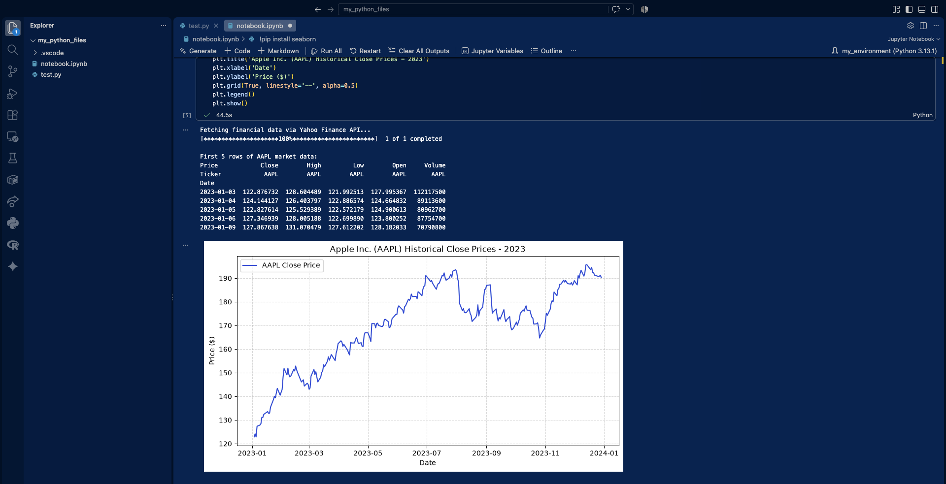
If the market dataset downloads and a clean line chart of Apple’s stock price appears, congratulations! You have successfully configured a professional, local Python environment for financial engineering.

This is how the output should look like if everything is working correctly:

An image of the VS Code menu with notebook.ipynb and test.py created

Congratulations! You have successfully configured a professional, local Python environment, ready for financial engineering

A quick tip for installing additional packages

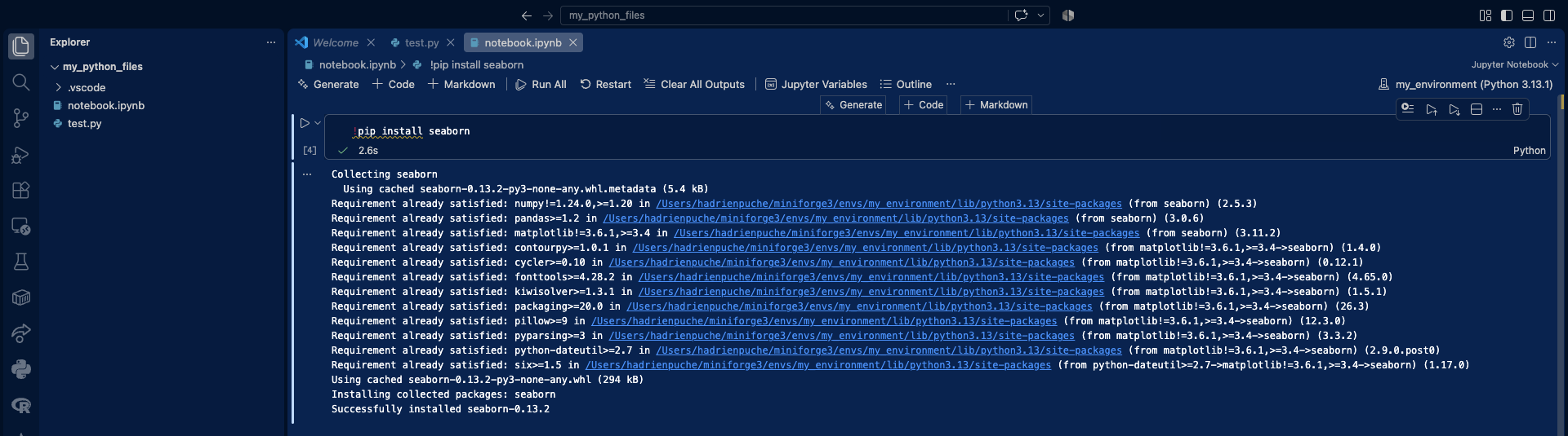
As you have seen, packages such as yfinance, matplotlib, and pandas extend Python with useful functionality for financial analysis. If you need to install an additional package while working in a Jupyter Notebook, you can use the %pip command directly in a notebook cell, provided that the appropriate Python environment is selected as the active kernel. For example, the following command installs seaborn, a high-level statistical data visualization library built on top of Matplotlib:

%pip install seaborn

An image of the VS Code menu with notebook.ipynb and test.py created

Next steps & financial use cases

Now that your environment is fully operational, you are ready to start applying Python to quantitative finance. Explore this article to learn how to use Python to download and use financial market data.

   ▶ Hadrien Puche How to download and model financial data with Python

If you are interested in programming languages and would like to learn another useful skill, explore these two articles about how you could use the programming language R to help you in your financial analysis:

   ▶ Hadrien Puche How to install and run R on your computer (A step-by-step guide)

   ▶ Hadrien Puche How to download financial data with R

About the Author

This article was written in September 2026 by Hadrien PUCHE (ESSEC Business School, Grande École Program, Master in Management, 2023-2027).

   ▶ Discover all posts by Hadrien PUCHE
How to get crypto data

How to get crypto data

 Snehasish CHINARA

In this article, Snehasish CHINARA (ESSEC Business School, Grande Ecole Program – Master in Management, 2022-2024) explains how to get crypto data.

Types of data

Number of coins

The information on the number of coins in circulation for a given currency is important to compute its market capitalization. Market capitalization is calculated by multiplying the current price of the cryptocurrency by its circulating number of coins (supply). This metric gives a rough estimate of the cryptocurrency’s total value within the market and its relative size compared to other cryptocurrencies. A lower circulating supply often implies a greater level of scarcity and rarity.

For cryptocurrencies (unlike fiat money), the number of coins in circulation is given by a mathematical formula. The number of coins may be limited (like the Bitcoin) or unlimited (like Ethereum and Dogecoin) over time.

Cryptocurrencies with limited supplies, such as Bitcoin’s maximum supply of 21 million coins, can be perceived as more valuable due to their finite nature. Scarcity can contribute to investor interest and potential price appreciation over time. A lower circulating supply might indicate the potential for future adoption and value appreciation, as the limited supply can create scarcity-driven demand, especially if the cryptocurrency gains more utility and usage.

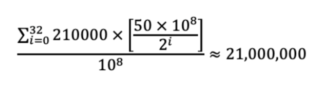
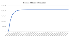
Bitcoin’s blockchain also relies on a key equation to steadily allow new BTC to be introduced. The equation below gives the total supply of bitcoins:

Total supply of bitcoins

Figure 1 below represents the evolution of the supply of Bitcoins.

Figure 1. Evolution of the supply of Bitcoins

Source: computation by the author.

Market price of a coin

The market price of a cryptocurrency in the market holds crucial insights into how well the cryptocurrency is faring. Although not the sole factor, the market price significantly contributes to evaluating the cryptocurrency’s performance and its prospects. The market price of a cryptocurrency is a dynamic and intricate element that reflects a multitude of factors, both intrinsic and extrinsic. The gradual rise in market value over time indicates a willingness among investors and traders to offer higher prices for the cryptocurrency. This signifies a rising interest and strong belief in the project’s potential for the future. The market price reflects the collective sentiment of investors and traders. Comparing the market price of a cryptocurrency to other similar cryptocurrencies or benchmark assets like Bitcoin can provide insights into its relative strength and performance within the market. A rising market price can indicate increasing adoption of the cryptocurrency for various use cases. Successful projects tend to attract more users and real-world applications, which can drive up the price.

The value of cryptocurrencies in the market is influenced by a variety of elements, with each factor contributing uniquely to their pricing. One of the most significant influences is market sentiment and investor psychology. These factors can cause prices to shift based on positive news, regulatory changes, or reactive selling due to fear. Furthermore, the real-world implementation and usage of a cryptocurrency are crucial for its prosperity. Concrete use cases such as Decentralized Finance (DeFi), Non-Fungible Tokens (NFTs), and international transactions play a vital role in creating demand and propelling price appreciation. Meanwhile, adherence to basic economic principles is evident in the supply-demand dynamics, where scarcity due to limited issuance, halving events, and token burns interact with the balance between supply and demand.

With the number of coins in circulation, the information on the price of coins for a given currency is also important to compute its market capitalization.

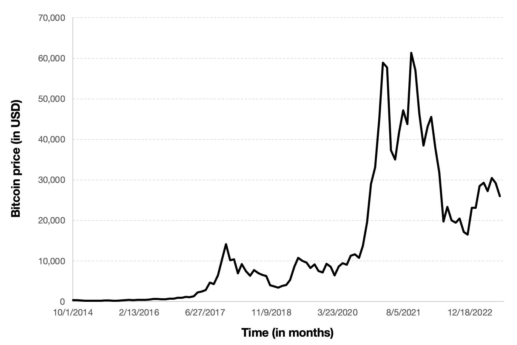
Figure 2 below represents the evolution of the price of Bitcoin in US dollar over the period October 2014 – August 2023. The price corresponds to the “closing” price (observed at 10:00 PM CET at the end of the month).

Figure 2. Evolution of the Bitcoin price
Evolution of the Bitcoin price
Source: computation by the author (data source: Yahoo! Finance).

Trading volume

Trading volume is crucial when assessing the health, reliability, and potential price movements of a cryptocurrency. Trading volume refers to the total amount of a cryptocurrency that is bought and sold within a specific time frame, typically measured in units of the cryptocurrency (e.g., BTC) or in terms of its equivalent value in another currency (e.g., USD).

Trading volume directly mirrors market liquidity, with higher volumes indicative of more liquid markets. This liquidity safeguards against drastic price fluctuations when trading, contrasting with low-volume scenarios that can breed volatility, where even a single substantial trade may disproportionately shift prices. Price alterations are most reliable and meaningful when accompanied by substantial trading volume. Price movements upheld by heightened volume often hold greater validity, potentially pointing to more pronounced market sentiment. When price surges parallel rising trading volume, it suggests a sustainable upward trajectory. Conversely, low trading volume amid rising prices may hint at a forthcoming correction or reversal. Scrutinizing the correlation between price oscillations and trading volume can uncover potential divergences. For instance, ascending prices coupled with dwindling trading volume may suggest a weakening trend.

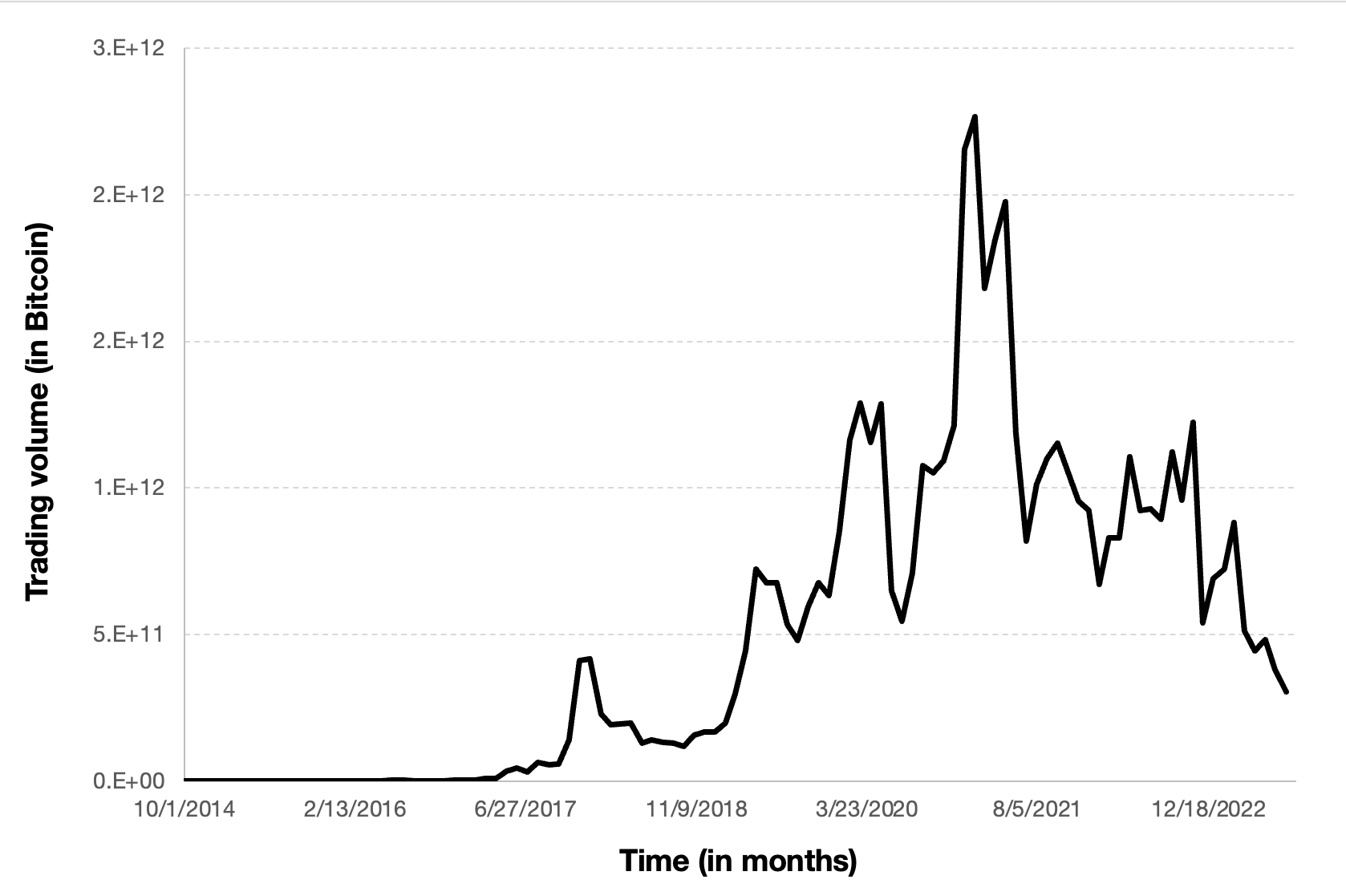
Figure 3 below represents the evolution of the monthly trading volume of Bitcoin over the period October 2014 – July 2023.

Figure 3. Evolution of the trading volume of Bitcoin
Evolution of the trading volume of Bitcoin
Source: computation by the author (data source: Yahoo! Finance).

Bitcoin data

You can download the Excel file with Bitcoin data used in this post as an illsutration.

Download the Excel file with Bitcoin data

Python code

You can download the Python code used to download the data from Yahoo! Finance.

Python script to download Bitcoin historical data and save it to an Excel sheet:

import yfinance as yf
import pandas as pd

# Define the ticker symbol and date range
ticker_symbol = “BTC-USD”
start_date = “2020-01-01”
end_date = “2023-01-01”

# Download historical data using yfinance
data = yf.download(ticker_symbol, start=start_date, end=end_date)

# Create a Pandas DataFrame
df = pd.DataFrame(data)

# Create a Pandas Excel writer object
excel_writer = pd.ExcelWriter(‘bitcoin_historical_data.xlsx’, engine=’openpyxl’)

# Write the DataFrame to an Excel sheet
df.to_excel(excel_writer, sheet_name=’Bitcoin Historical Data’)

# Save the Excel file
excel_writer.save()

print(“Data has been saved to bitcoin_historical_data.xlsx”)

# Make sure you have the required libraries installed and adjust the “start_date” and “end_date” variables to the desired date range for the historical data you want to download.

APIs

Calculating the total number of Bitcoins in circulation over time
Access – Bitcoin Blockchain data
By running a Bitcoin node or by using blockchain data providers like Blockchain.info, Blockchair, or a similar service.

Extract Block Data: Once you have access to the blockchain data, you would need to extract information from each block. Each block contains a record of the transactions that have occurred, including the creation (mining) of new Bitcoins in the form of a “Coinbase” transaction.

Calculate Cumulative Supply: You can calculate the cumulative supply of Bitcoins by adding up the rewards from each block’s Coinbase transaction. Initially, the block reward was 50 Bitcoins, but it halves approximately every four years due to the Bitcoin halving events. So, you’ll need to account for these halving in your calculations.

Code – python

import requests

# Replace ‘YOUR_API_KEY’ with your CoinMarketCap API key
api_key = ‘YOUR_API_KEY’

# Define the endpoint URL for CoinMarketCap’s API
url = ‘https://pro-api.coinmarketcap.com/v1/cryptocurrency/quotes/latest’

# Define the parameters for the request
params = {
‘symbol’: ‘BTC’,
‘convert’: ‘USD’,
‘CMC_PRO_API_KEY’: api_key
}

# Send the request to CoinMarketCap
response = requests.get(url, params=params)

# Parse the response JSON
data = response.json()

# Extract the circulating supply from the response
circulating_supply = data[‘data’][‘BTC’][‘circulating_supply’]

print(f”Current circulating supply of Bitcoin: {circulating_supply} BTC”)

## Replace ‘YOUR_API_KEY’ with your actual CoinMarketCap API key.

Why should I be interested in this post?

Cryptocurrency data is becoming increasingly relevant in these fields, offering opportunities for research, data analysis skill development, and even career prospects. Whether you’re aiming to conduct research, stay informed about the evolving financial landscape, or simply enhance your data analysis abilities, understanding how to access and work with crypto data is an asset. Plus, as the cryptocurrency industry continues to grow, this knowledge can open new career paths and improve your personal finance decision-making. In a rapidly changing world, diversifying your knowledge with cryptocurrency data acquisition skills can be a wise investment in your future.

Related posts on the SimTrade blog

▶ Alexandre VERLET Cryptocurrencies

▶ Youssef EL QAMCAOUI Decentralised Financing

▶ Hugo MEYER The regulation of cryptocurrencies: what are we talking about?

Useful resources

APIs

CoinMarketCap Source of API keys and program

CoinGecko Source of API keys and Programs

CryptoNews Source of API keys and Programs

Data sources

Yahoo! Finance Historical data for Bitcoin

Coinmarketcap Historical data for Bitcoin

Blockchain.com Market Data and charts on Bitcoin history

About the author

The article was written in October 2023 by Snehasish CHINARA (ESSEC Business School, Grande Ecole Program – Master in Management, (2022-2024).

Programming Languages for Quants

Jayati WALIA

In this article, Jayati WALIA (ESSEC Business School, Grande Ecole Program – Master in Management, 2019-2022) presents an overview of popular programming languages used in quantitative finance.

Introduction

Finance as an industry has always been very responsive to new technologies. The past decades have witnessed the inclusion of innovative technologies, platforms, mathematical models and sophisticated algorithms solve to finance problems. With tremendous data and money involved and low risk-tolerance, finance is becoming more and more technological and data science, blockchain and artificial intelligence are taking over major decision-making strategies by the power of high processing computer algorithms that enable us to analyze enormous data and run model simulations within nanoseconds with high precision.

This is exactly why programming is a skill which is increasingly in demand. Programming is needed to analyze financial data, compute financial prices (like options or structured products), estimate financial risk measures (like VaR) and test investment strategies, etc. Now we will see an overview of popular programming languages used in modelling and solving problems in the quantitative finance domain.

Python

Python is general purpose dynamic high level programming language (HLL). It’s effortless readability and straightforward syntax allows not just the concept to be expressed in relatively fewer lines of code but also makes it’s learning curve less steep.

Python possesses some excellent libraries for mathematical applications like statistics and quantitative functions such as numpy, scipy and scikit-learn along with the plethora of accessible open source libraries that add to its overall appeal. It supports multiple programming approaches such as object-oriented, functional, and procedural styles.

Python is most popular for data science, machine learning and AI applications. With data science becoming crucial in the financial services industry, it has consequently created an immense demand for Python, making it a programming language of top choice.

C++

The finance world has been dominated by C++ for valid reasons. C++ is one of the essential programming languages in the fintech industry owing to its execution speed. Developers can leverage C++ when they need to programme with advanced computations with low latency in order to process multiple functions fasters such as in High Frequency Trading (HFT) systems. This language offers code reusability (which is crucial in multiple complex quantitative finance projects) to programmers with a diverse library comprising of various tools to execute.

Java

Java is known for its reliability, security and logical architecture with its object-oriented programming to solve complicated problems in the finance domain. Java is heavily used in the sell-side operations of finance involving projects with complex infrastructures and exceptionally robust security demands to run on native as well as cross-platform tools. This language can help manage enormous sets of real-time data with the impeccable security in bookkeeping activity. Financial institutions, particularly investment banks, use Java and C# extensively for their entire trading architecture, including front-end trading interfaces, live data feeds and at times derivatives’ pricing.

R

R is an open source scripting language mostly used for statistical computing, data analytics and visualization along with scientific research and data science. R the most popular language among mathematical data miners, researchers, and statisticians. R runs and compiles on multiple platforms such as Unix, Windows and MacOS. However, it is not the easiest of languages to learn and uses command line scripting which may be complex to code for some.

Scala

Scala is a widely used programming language in banks with Morgan Stanley, Deutsche Bank, JP Morgan and HSBC are among many. Scala is particularly appropriate for banks’ front office engineering needs requiring functional programming (programs using only pure functions that are functions that always return an immutable result). Scala provides support for both object-oriented and functional programming. It is a powerful language with an elegant syntax.

Haskell and Julia

Haskell is a functional and general-purpose programming language with user-friendly syntax, and a wide collection of real-world libraries for user to develop the quant solving application using this language. The major advantage of Haskell is that it has high performance, is robust and is useful for modelling mathematical problems and programming language research.

Julia, on the other hand, is a dynamic language for technical computing. It is suitable for numerical computing, dynamic modelling, algorithmic trading, and risk analysis. It has a sophisticated compiler, numerical accuracy with precision along with a functional mathematical library. It also has a multiple dispatch functionality which can help define function behavior across various argument combinations. Julia communities also provide a powerful browser-based graphical notebook interface to code.

Related posts on the SimTrade blog

▶ Jayati WALIA Quantitative Finance

▶ Jayati WALIA Quantitative Risk Management

▶ Jayati WALIA Value at Risk

▶ Akshit GUPTA The Black-Scholes-Merton model

Useful Resources

Websites

QuantInsti Python for Trading

Bankers by Day Programming languages in FinTech

Julia Computing Julia for Finance

R Examples R Basics

About the author

The article was written in October 2021 by Jayati WALIA (ESSEC Business School, Grande Ecole Program – Master in Management, 2019-2022).