

In this article, Youssef LOURAOUI (Bayes Business School, MSc. Energy, Trade & Finance, 2021-2022) presents the Capital Market Line (CML), a key concept in asset pricing derived from the Capital Asset Pricing Model (CAPM).
This article is structured as follows: we first introduce the concept. We then illustrate how to estimate the capital market line (CML). We finish by presenting the mathematical foundations of the CML.
Capital Market Line
An optimal portfolio is a set of assets that maximizes the trade-off between expected return and risk: for a given level of risk, the portfolio with the highest expected return, or for a given level of expected return, the portfolio with the lowest risk.
Let us consider two cases: 1) when investors have access to risky assets only; 2) when investors have access to risky assets and a risk-free asset (earning a constant interest rate, 2% for example below).
Risky assets
In the case of risky assets only, the efficient frontier (the set of optimal portfolios) is represented below in Figure 1.
Figure 1. Efficient frontier with risky assets only.
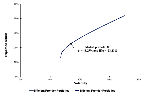
Source: Computation by the author.
Risky assets and a risk-free asset
In the case of risky assets and a risk-free asset, the efficient frontier (the set of optimal portfolios) is represented below in Figure 2. In this case, the efficient frontier is a straight line called the Capital Market Line (CML).
Figure 2. Efficient frontier with risky assets and a risk-free asset.
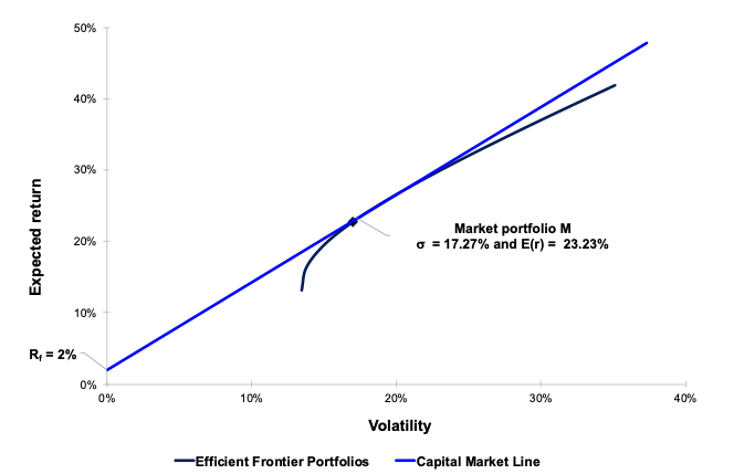
Source: Computation by the author.
The CML joins the risk-free asset and the tangency portfolio, which is the intersection with the efficient frontier with risky assets only. We can reasonably conclude from Figure 2 that, to increase expected return, an investor has to increase the amount of risk he or she takes to attain returns higher than the risk-free interest rate. As a result, the Sharpe ratio of the market portfolio equals the slope of the CML. If the Sharpe ratio is more than the CML, an investment strategy can be implemented, such as buying assets if the Sharpe ratio is greater than the CML and selling assets if the Sharpe ratio is less than the CML (Drake and Fabozzi, 2011).
Investors who allocate their money between a riskless asset and the risky market portfolio M can expect a return equal to the risk-free rate plus compensation for the number of risk units σP) they accept. This result is in line with the underlying notion of all investment theory: investors perform two services in the capital markets for which they might expect to be compensated. First, they enable someone else to utilize their money in exchange for a risk-free interest rate. Second, they face the risk of not receiving the promised returns in exchange for their invested capital. The term E(rM)- Rf) / σM refers to the investor’s expected risk premium per unit of risk, which is also known as the expected compensation per unit of risk taken.
Figure 3 represents the Capital Market Line which connect the risk-free asset to the efficient frontier line. The straight line in Figure 3 represents a combination of a risky portfolio and a riskless asset. Any combination of the risk-free asset and Portfolio A is similarly outperformed by some combination of the risk-free asset and Portfolio B. Continue drawing a line from Rf to the efficient frontier with increasing slopes until you reach Portfolio M’s point of tangency. All other possible portfolio combinations that investors could build are outperformed by the collection of portfolio possibilities along Line Rf-M, which is the CML. The CML, in this sense, represents a new efficient frontier that combines the Markowitz efficient frontier of risky assets with the ability to invest in risk-free securities. The CML’s slope is (E(rM)- Rf) / σ(M), which is the highest risk premium compensation that investors can expect for each unit of risk they take on (Reilly and Brown, 2012) (Figure 3).
If we fully invest our cash on the risk-free rate, we would be exactly on the y axis with an expected return of 2%. Each time we move along the curve that connects the risk-free rate to the optimum market portfolio, we allocate less weight to the risk-free rate, and we overweight more on riskier assets (Point A). Points M represents the optimal risky portfolio in the efficient frontier line, which minimizes the overall portfolio variance. It would have a weighting of 45% in stock A and a 55% in stock B, which would offer a 26.23% annualized return for a 17.27% annualized volatility. Point B represents a portfolio composition that is based on a leveraged position of 140% on the optimal risky portfolio and a short position on the risk-free asset of -40% (Figure 3).
Figure 3. Efficient frontier with different points.
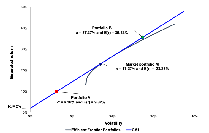
Source: Computation by the author.
Mathematical representation
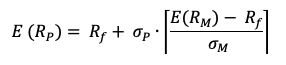
We can define the CML as the line that is tangent to the efficient frontier which connects the risk-free asset with the market portfolio:
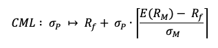
Where:
- σP: the volatility of portfolio P
- Rf: the risk-free interest rate
- E(RM): the expected return of the market M
- σM: the volatility of the market M
- E[RM– Rf]: the market risk premium.
The expected return of the portfolio can be computed as:
The Sharpe Ratio is shown in parenthesis, and it compares the performance of an investment, such as a security or portfolio, to the performance of a risk-free asset after adjusting for risk. It is calculated by dividing the difference between the investment returns and the risk-free return by the standard deviation of the investment returns. It denotes the additional amount of return that an investor receives for each unit of risk increase (Sharpe, 1963). We can define it mathematically as:
We can identify the following relationship between the slope of the CML and the Sharpe ratio of the market portfolio, defined mathematically as follows:
A simple strategy for stock selection is to buy assets with Sharpe ratios that are higher than the CML and sell those with Sharpe ratios that are lower. Indeed, the efficient market hypothesis implies that beating the market is impossible. As a result, all portfolios should have a Sharpe ratio that is lower than or equal to the market. As a result, if a portfolio (or asset) has a higher Sharpe ratio than the market, this portfolio (or asset) has a higher return per unit of risk (i.e. volatility), which contradicts the efficient market hypothesis. The alpha is the abnormal excess return over the market return at a given level of risk.
Why should I be interested in this post?
Sharpe ratio is a popular tool for assessing portfolio risk/return in finance. The Sharpe ratio informs the investor precisely which portfolio has the best performance among the available options. This simplifies the investor’s decision-making process. The higher the ratio, the greater the return for each unit of risk.
If you are a business school or university undergraduate or graduate student, this content will help you in broadening your knowledge of finance.
Related posts on the SimTrade blog
▶ Youssef LOURAOUI Portfolio
▶ Youssef LOURAOUI Systematic and Specific risk
▶ Jayati WALIA Capital Asset Pricing Model (CAPM)
▶ Youssef LOURAOUI Markowitz Modern Portfolio Theory
▶ Youssef LOURAOUI Alpha
▶ Youssef LOURAOUI Factor Investing
▶ Youssef LOURAOUI Origin of factor investing
▶ Youssef LOURAOUI Security Market Line (SML)
Useful resources
Academic research
Pamela, D. and Fabozzi, F., 2010. The Basics of Finance: An Introduction to Financial Markets, Business Finance, and Portfolio Management. John Wiley and Sons Edition.
Lintner, J. 1965a. The Valuation of Risk Assets and the Selection of Risky Investments in Stock Portfolios and Capital Budgets. The Review of Economics and Statistics 47(1): 13-37.
Lintner, J. 1965b. Security Prices, Risk and Maximal Gains from Diversification. The Journal of Finance, 20(4): 587-615.
Mossin, J. 1966. Equilibrium in a Capital Asset Market. Econometrica, 34(4): 768-783.
Reilly, R. K., Brown C. K., 2012. Investment Analysis & Portfolio Management, Tenth Edition.
Sharpe, W.F. 1963. A Simplified Model for Portfolio Analysis. Management Science, 9(2): 277-293.
Sharpe, W.F. 1964. Capital Asset Prices: A Theory of Market Equilibrium under Conditions of Risk. The Journal of Finance, 19(3): 425-442.
About the author
The article was written in November 2021 by Youssef LOURAOUI (Bayes Business School, MSc. Energy, Trade & Finance, 2021-2022).