In this article, Youssef LOURAOUI (Bayes Business School, MSc. Energy, Trade & Finance, 2021-2022) elaborates on the concept of alpha, one of the fundamental parameters for portfolio performance measure.
This article is structured as follows: we introduce the concept of alpha in asset management. Next, we present some interesting academic findings on the alpha. We finish by presenting the mathematical foundations of the concept.
Introduction
The alpha (also called Jensen’s alpha) is defined as the additional return delivered by the fund manager on the overall performance of the portfolio compared to the market performance (Jensen, 1968). A key issue in finance (and particularly in portfolio management) has been evaluating the performance of portfolio managers. The term ‘performance’ encompasses at least two independent dimensions (Sharpe, 1967): 1) The portfolio manager’s ability to boost portfolio returns by successful forecasting of future security prices; and 2) The portfolio manager’s ability to minimize (via “efficient” diversification) the amount of “insurable risk” borne by portfolio holders.
The primary hurdle to evaluating a portfolio’s performance in these two categories has been a lack of a solid grasp of the nature and assessment of “risk”. Risk aversion appears to predominate in the capital markets, and as long as investors accurately perceive the “riskiness” of various assets, this indicates that “risky” assets must on average give higher returns than less “risky” assets. Thus, when evaluating portfolios’ performance, the implications of varying degrees of risk on their returns must be considered (Sharpe, 1967).
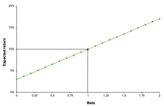
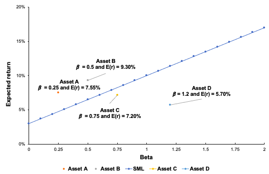
One way of representing the performance is by linking the performance of a portfolio to the security market line (SML). Figure 1 depicts the relation between the portfolio performance in relation to the security market line. As illustrated in Figure 1 below, Fund A has a negative alpha as it is located under the SML, implying a negative performance of the fund manager compared to the market. Fund B has a positive alpha as it is located above the SML, implying a positive performance of the fund manager compared to the market.
Figure 1. Alpha and the Security Market Line
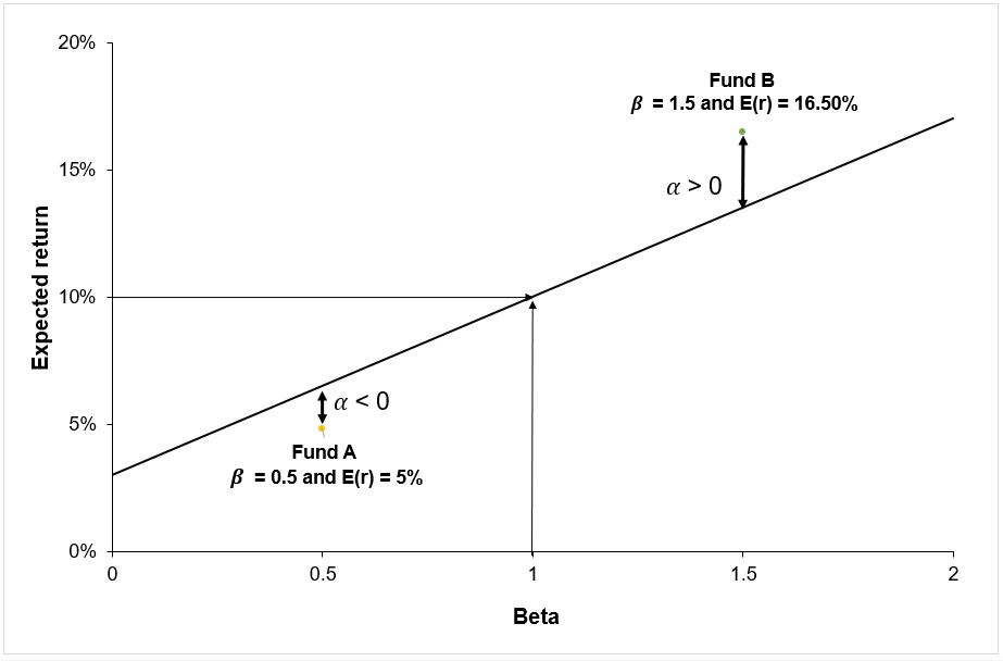
Source: Computation by the author.
You can download below an Excel file with data to compute Jensen’s alpha for fund performance analysis.

Academic Literature
Jensen develops a risk-adjusted measure of portfolio performance that quantifies the contribution of a manager’s forecasting ability to the fund’s returns. In the first empirical study to assess the outperformance of fund managers, Jensen aimed at quantifying the predictive ability of 115 mutual fund managers from 1945 to 1964. He looked at their ability to produce returns above the expected return given the risk level of each portfolio. Not only does the evidence on mutual fund performance indicate that these 115 funds on average were unable to forecast security prices accurately enough to outperform a buy-and-hold strategy, but there is also very little evidence that any individual fund performed significantly better than what we would expect from mutual random chance. Additionally, it is critical to highlight that these conclusions hold even when fund returns are measured net of management expenses (that is assume their bookkeeping, research, and other expenses except brokerage commissions were obtained free). Thus, on average, the funds did not appear to be profitable enough in their trading activity to cover even their brokerage expenses.
Mathematical derivation of Jensen’s alpha
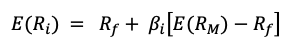
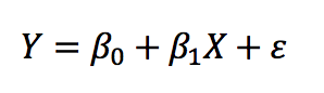
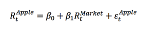
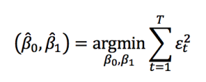
The portfolio performance metric given below is derived directly from the theoretical results of Sharpe (1964), Lintner (1965a), and Treynor (1965) capital asset pricing models. All three models assume that (1) all investors are risk-averse and single-period expected utility maximizers, (2) all investors have identical decision horizons and homogeneous expectations about investment opportunities, (3) all investors can choose between portfolios solely based on expected returns and variance of returns, (4) all transaction costs and taxes are zero, and (5) all assets are infinitely fungible. With the extra assumption of an equilibrium capital market, each of the three models produces the following equation for the expected one-period return defined by (Jensen, 1968):
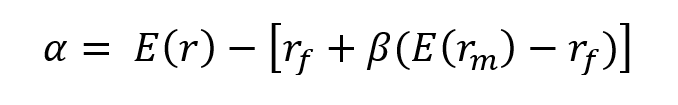
- E(r): the expected return of the fund
- rf: the risk-free rate
- E(rm): the expected return of the market
- β(E(rm) – rf): the systematic risk of the portfolio
- α: the alpha of the portfolio (Jensen’s alpha)
Why should I be interested in this post?
If you are a business school or university student, this post will help you to understand the fundamentals of investment.
Related posts on the SimTrade blog
▶ Youssef LOURAOUI Portfolio
▶ Youssef LOURAOUI Systematic risk and specific risk
▶ Youssef LOURAOUI Beta
▶ Youssef LOURAOUI Markowitz Modern Portfolio Theory
▶ Jayati WALIA. Capital Asset Pricing Model (CAPM)
Useful resources
Academic research
Fama, Eugene F. 1965. The Behavior of Stock Market Prices.Journal of Business 37, 34-105.
Fama, Eugene F. 1967. Risk, Return, and General Equilibrium in a Stable Paretian Market. Chicago, IL: University of Chicago.Unpublished manuscript.
Fama, Eugene F. 1968. Risk, Return, and Equilibrium: Some Clarifying Comments. Journal of Finance, 23, 29-40.
Lintner, John. 1965a. Security Prices, Risk, and Maximal Gains from Diversification. Journal of Finance, 20, 587-616.
Lintner, John. 1965b. The Valuation of Risk Assets and the Selection of Risky Investments in Stock Portfolios and Capital Budgets.Review of Economics and Statistics 47, 13-37.
Markowitz, H., 1952. Portfolio Selection. The Journal of Finance, 7, 77-91.
Sharpe, William F. 1963. A Simplified Model for Portfolio Analysis. Management Science, 19, 425-442.
Sharpe, William F. 1964. Capital Asset Prices: A Theory of Market Equilibrium under Conditions of Risk. Journal of Finance, 19, 425-442.
Sharpe, William F. 1966. Mutual Fund Performance. Journal of Business39, Part 2: 119-138.
Treynor, Jack L. 1965. How to Rate Management of Investment Funds.Harvard Business Review 18, 63-75.
Business analysis
JP Morgan Asset Management, 2021.Glossary of investment terms: Alpha
About the author
The article was written in November 2021 by Youssef LOURAOUI (Bayes Business School,, MSc. Energy, Trade & Finance, 2021-2022).