

This article written by Akshit GUPTA (ESSEC Business School, Grande Ecole Program – Master in Management, 2019-2022) presents the Black-Scholes-Merton Model .
Introduction
Options are one of the most popular derivative contracts used by investors to hedge the risks of their portfolios, to optimize the risk profile of their positions and to make profits (or losses) by means of speculation. The value of options is known at maturity date (or expiration date) as it is given by their pay-off functions defined in their contracts. But what is the value of the option at the issuance date or any date between the issuance and the expiration? The Black-Scholes-Merton model allows to answer this question.
The Black-Scholes-Merton model is an continuous-time option pricing model used to determine the fair price or theoretical value for a call or a put option based on variable factors such as the maturity date and the strike price of the option (option characteristics), and the price of underlying asset, the volatility of the price of underlying asset, and the risk-free rate (market data). It is used to determine the price of a European call option, which refers to the option that can only be exercised on the maturity date.
History
The model was first introduced to the world by a paper titled ‘The Pricing of Options and Corporate Liabilities’ by Fischer Black and Myron Scholes and was officially published in spring 1973. Almost around the same time as Black and Scholes, Robert Merton, who was also a colleague of Scholes at MIT Sloan, presented his contributions to the model in another paper named ‘Theory of Rational Option Pricing’, where he coined the name “Black-Scholes model”. Later, Black and Scholes also published empirical tests of the model in their ‘The Valuation of Option Contracts and a Test of Market Efficiency’ paper. For their significant contribution to the world of financial markets, Merton and Black were awarded the prestigious Nobel Prize in Economic Sciences in 1997 (unfortunately Scholes had passed away in 1995 due to which he was ineligible for the Nobel Prize).
In the BSM model, the value of an option depends on the future volatility of the underlying stock rather than on its expected return. The pricing formula is based on the assumption that the price of the underlying asset follows a geometric Brownian motion.
Option pricing with BSM
The BSM model is used to find the theoretical value of a European option. The model assumes that the price of the underlying asset follows a geometric Brownian motion, which implies that the returns on the underlying asset are normally distributed. It is also assumed that there are no arbitrage opportunities, no transaction costs and the risk-free rate remains constant over time.
The BSM formula
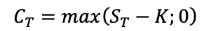
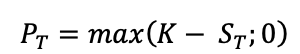
The payoffs for a call option and a put option give the value of these options at the maturity date T:
For a call option:
For a put option:
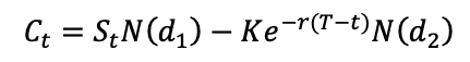
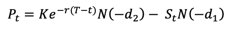
The BSM formula gives the price of European put and call options at any date before the maturity date T. The value of European call and put options for a non-dividend paying stock are given by:
For a call option:
For a put option:
where,
The notations used in the above formulae are described as :
St: price of the underlying asset at time t
t: current date (or date of calculation of option price)
T: maturity or expiry date of the option
K: strike price of the option
r: risk-free interest rate
σ: volatility (the standard deviation of the return on the underlying asset)
N(.): cumulative distribution function for a normal (Gaussian) distribution (0 ≤ N(.) ≤ 1 )
For a call option, N(+d2) is the probability that the option will be exercised, and Ke(-r(T-t) ) N(+d2) is what is expected to be paid for the underlying stock if the option is exercised, discounted to today (or the calculation date t).
Similarly, SN(+d1) is what we can expect to receive from selling the underlying stock, if the option is exercised, also discounted to today (or the calculation date t).
For a put option, N(-d2) is the probability that the option will be exercised, and Ke(-r(T-t) ) N(-d1 ) is what is expected to be paid for the underlying stock if the option is exercised, discounted to today (or the calculation date t).
Similarly, SN(-d1 ) is what we can expect to receive from selling the underlying stock, if the option is exercised, also discounted to today (or the calculation date t).
Note that the value of the option given by the BSM formula depends on the maturity date and the strike price of the option (option characteristics), and the price of underlying asset, and the risk-free rate (market data) and the volatility of the price of underlying asset. While the option characteristics are known and the market data are observable, the volatility of the price of underlying asset is the only unknown variable in the formula.
Beyond the formula itself for the option prices, the BSM model also gives a method to manage the option over time (delta hedging) as an option is equivalent (under the assumption of no arbitrage) to a portfolio composed of the underlying asset and risk-free bond.
Example – Call and Put option pricing using Black-Scholes-Merton model
Figure 1 gives the graphical representation of the value of a call option at time t as a function of the price of the underlying asset at time t as given by the BSM formula. The strike price for the call option is 40€ with a maturity of 0.50 years. The price of the underlying asset is 50€ at time t and volatility is 40%. The risk-free rate is assumed to be 1%.
Figure 1. Call option Pricing using BSM formula 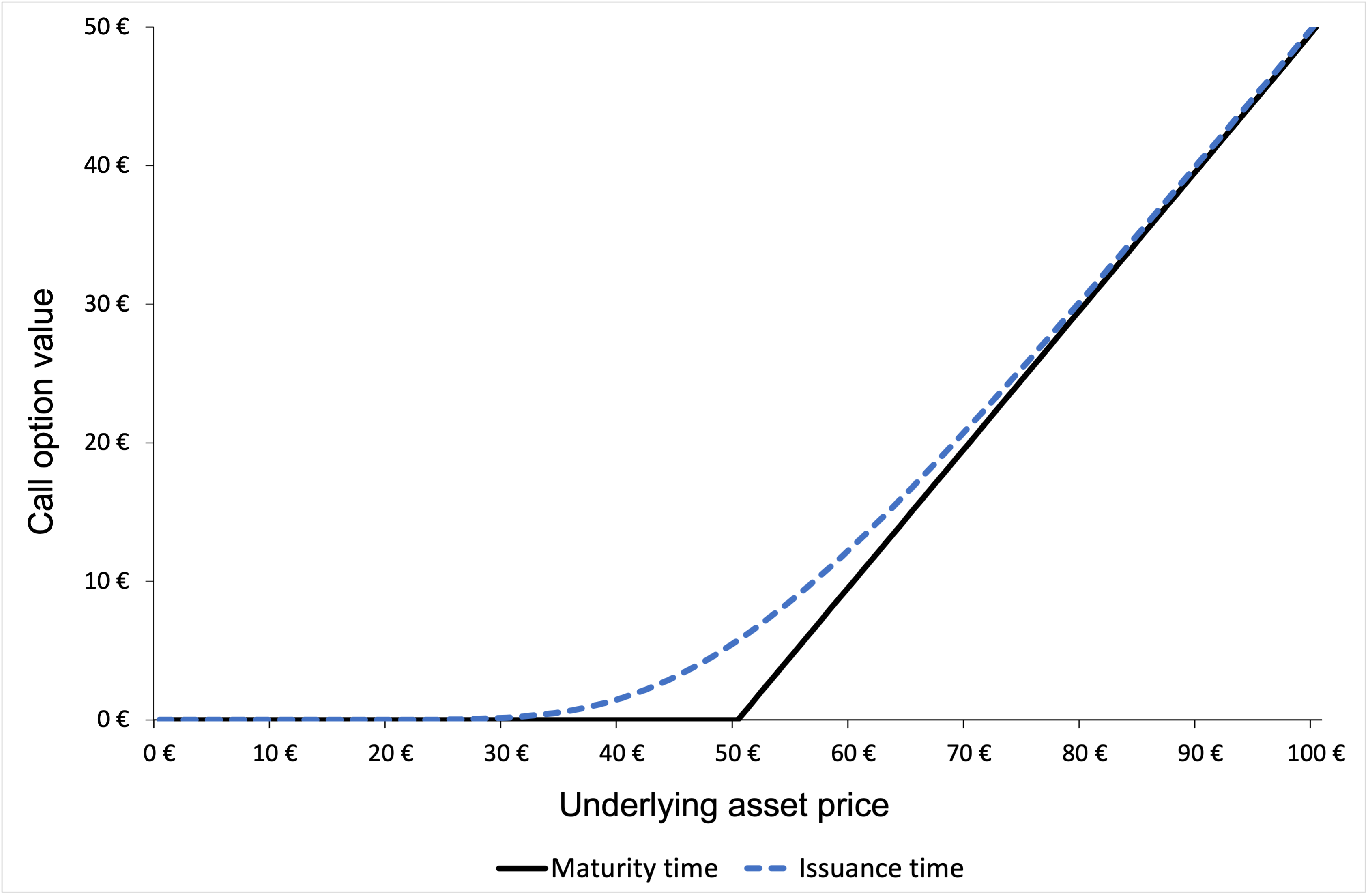
Source: computation by the author (based on the BSM model).
Figure 2 gives the graphical representation of the value of a put option at time t as a function of the price of the underlying asset at time t as given by the BSM formula. The strike price for the put option is 40€ with a maturity of 0.50 years. The price of the underlying asset is 50€ at time t and volatility is 40%. The risk-free rate is assumed to be 1%.
Figure 2. Put option Pricing using BSM formula 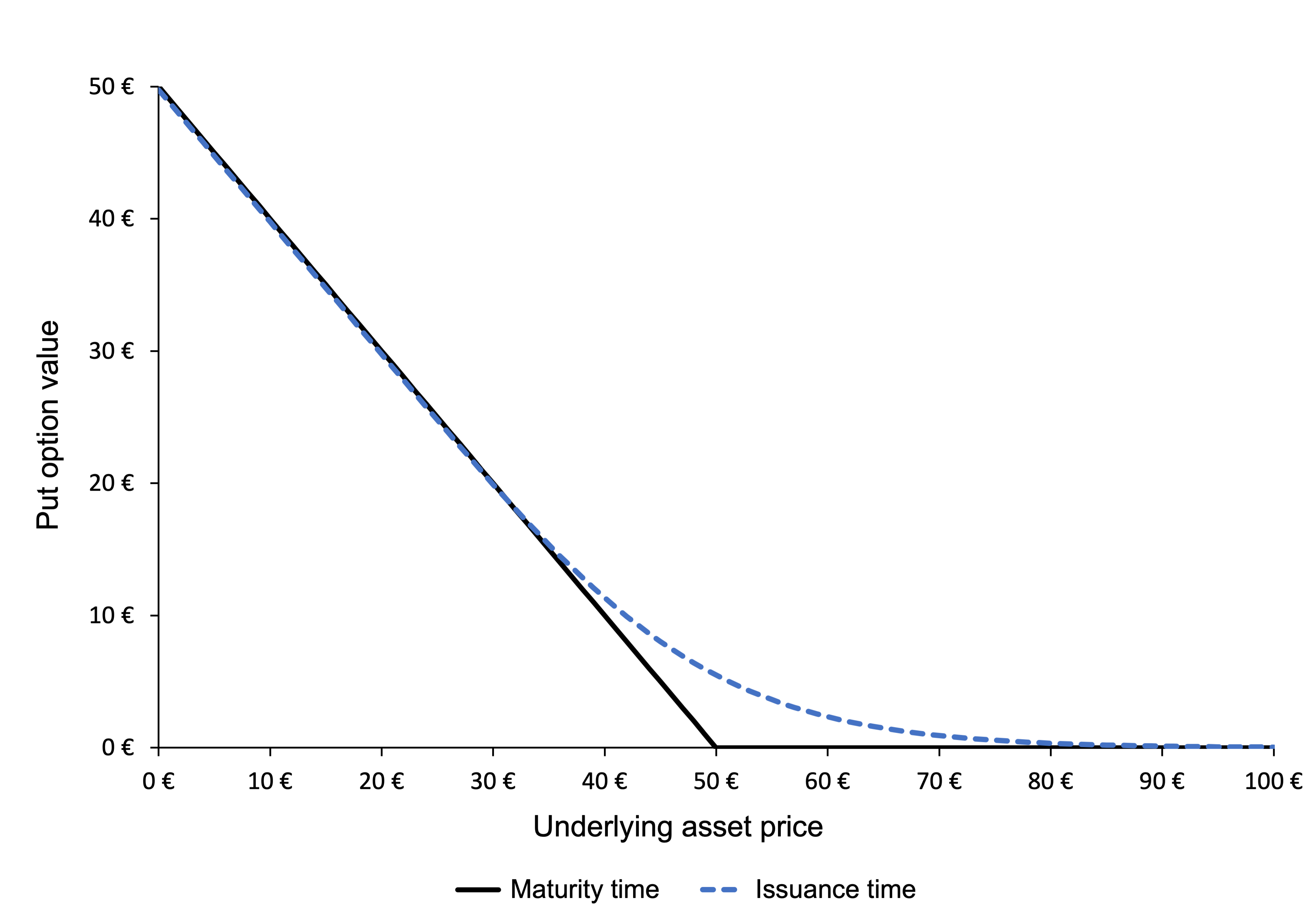
Source: computation by the author (based on the BSM model).
You can download below the Excel file used for the computation of the Call and Put option prices using the BSM Model.

Conclusion
The option-pricing model developed by Black, Scholes and Merton in 1973 provides a way of computing the prices of option contracts and has been widely used by traders since its publication. Following the seminal works by Black, Scholes and Merton, there haven been many extensions of their model, which have broadened its applicability to other instruments such as more complex options and insurance contracts.
Limitations of the BSM model
However, the model is sometimes criticized due to its weaknesses emerging from unrealistic sets of assumptions, which cause errors in estimation and model’s predictions. For instance, the BSM model assumes a constant value for volatility of the price of the underlying asset and also neglects any dividend payments from stocks which is certainly not the case in real life. Also, the model is only applicable to European options and would not be able to accurately determine the value of an American option which can be exercised at any time until the expiry date. Researchers have worked on amending the model to incorporate more realistic assumptions and have concluded that despite the model’s weaknesses, its application is still extremely useful in analyzing option prices.
Related posts on the SimTrade blog
▶ Jayati WALIA Black-Scholes-Merton option pricing model
▶ Akshit GUPTA Options
▶ Akshit GUPTA History of Options markets
▶ Akshit GUPTA Option Trader – Job description
Useful resources
Academic research
Black F. and M. Scholes (1973) “The Pricing of Options and Corporate Liabilities” The Journal of Political Economy, 81, 637-654.
Hull J.C. (2015) Options, Futures, and Other Derivatives, Ninth Edition, Chapter 15 – The Black-Scholes-Merton model, 343-375.
Merton R.C. (1973) “Theory of Rational Option Pricing” Bell Journal of Economics, 4, 141–183.
Wilmott P. (2007) Paul Wilmott Introduces Quantitative Finance, Second Edition, Chapter 8 – The Black Scholes Formula and The Greeks, 182-184.
About the author
Article written in August 2021 by Akshit GUPTA (ESSEC Business School, Grande Ecole Program – Master in Management, 2019-2022).