The Nikkei 225 index

In this article, Nithisha CHALLA (ESSEC Business School, Grande Ecole Program – Master in Management, 2021-2023) presents the Nikkei 225 index and details its characteristics.
The Nikkei 225 index
The Nikkei 225 index is considered as the primary benchmark index of the Tokyo Stock Exchange (TSE) and is the most widely quoted average of Japanese equities. One of Japan’s top newspapers, the Nihon Keizai Shimbun (Nikkei), first published the index in 1950. The index consists of 225 blue-chip companies listed on the TSE, which are considered to represent the overall health of the Japanese economy. These companies come from various industries such as finance, technology, automobile, and retail, among others.
The Financial Times, a preeminent global provider of financial news, was purchased by Nikkei Inc, the parent company of Nikkei, for $1.3 billion in 2015. This acquisition highlighted Nikkei’s growing global presence and ambition to diversify beyond the Japanese market. The Nikkei 225 index follows a price-weighted methodology. This means that the components of the index are weighted based on their stock price, with higher-priced stocks carrying a greater weight in the index.
In the past few years, the Nikkei 225 index has been affected by various economic and political events, such as the COVID-19 pandemic and the Tokyo Olympics. The pandemic caused the index to significantly decline in 2020, but it has since recovered and reached new highs in 2021.
How is the Nikkei 225 index represented in trading platforms and financial websites? The ticker symbol used in the financial industry for the Nikkei 225 index is “NI225”.
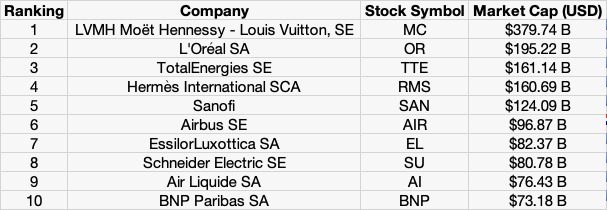
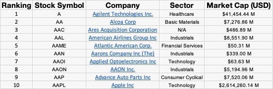
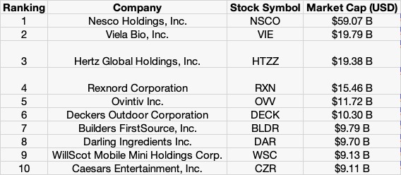
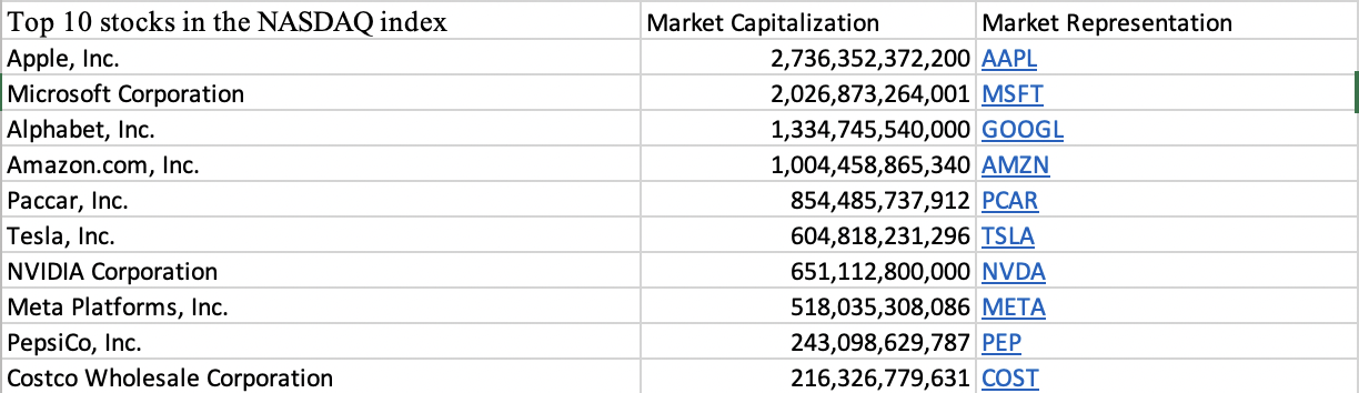
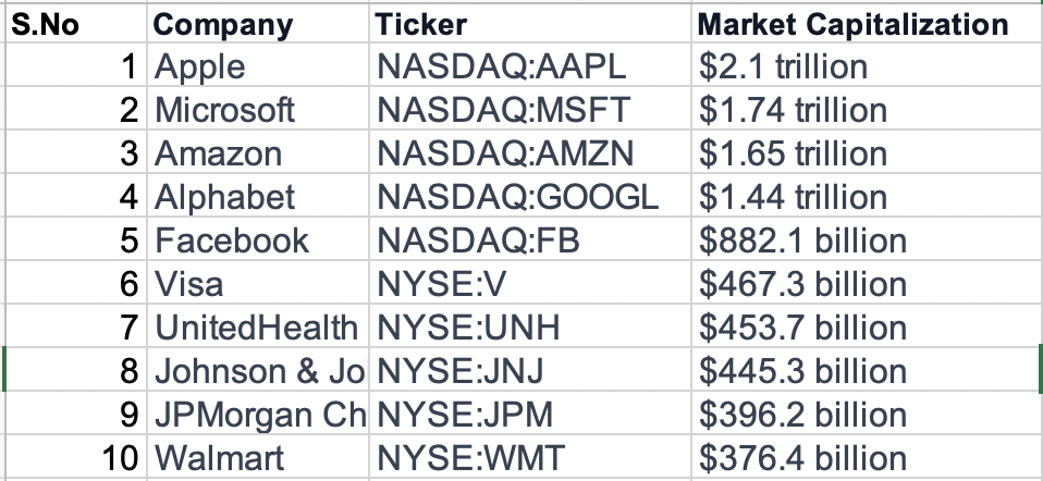
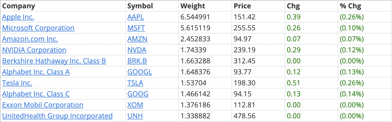
Table 1 below gives the Top 10 stocks in the Nikkei 225 index in terms of market capitalization as of January 31, 2023.
Table 1. Top 10 stocks in the Nikkei index.
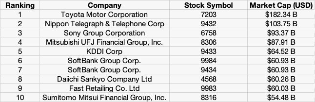
Source: computation by the author (data: YahooFinance! financial website).
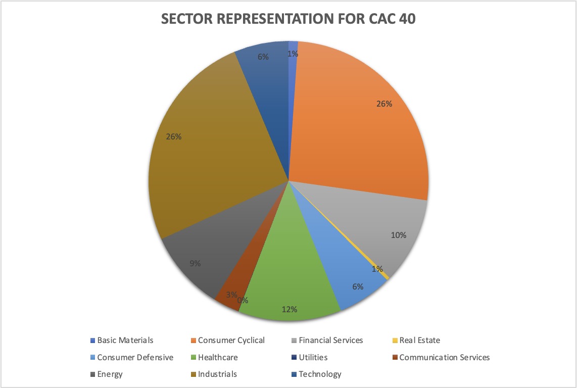
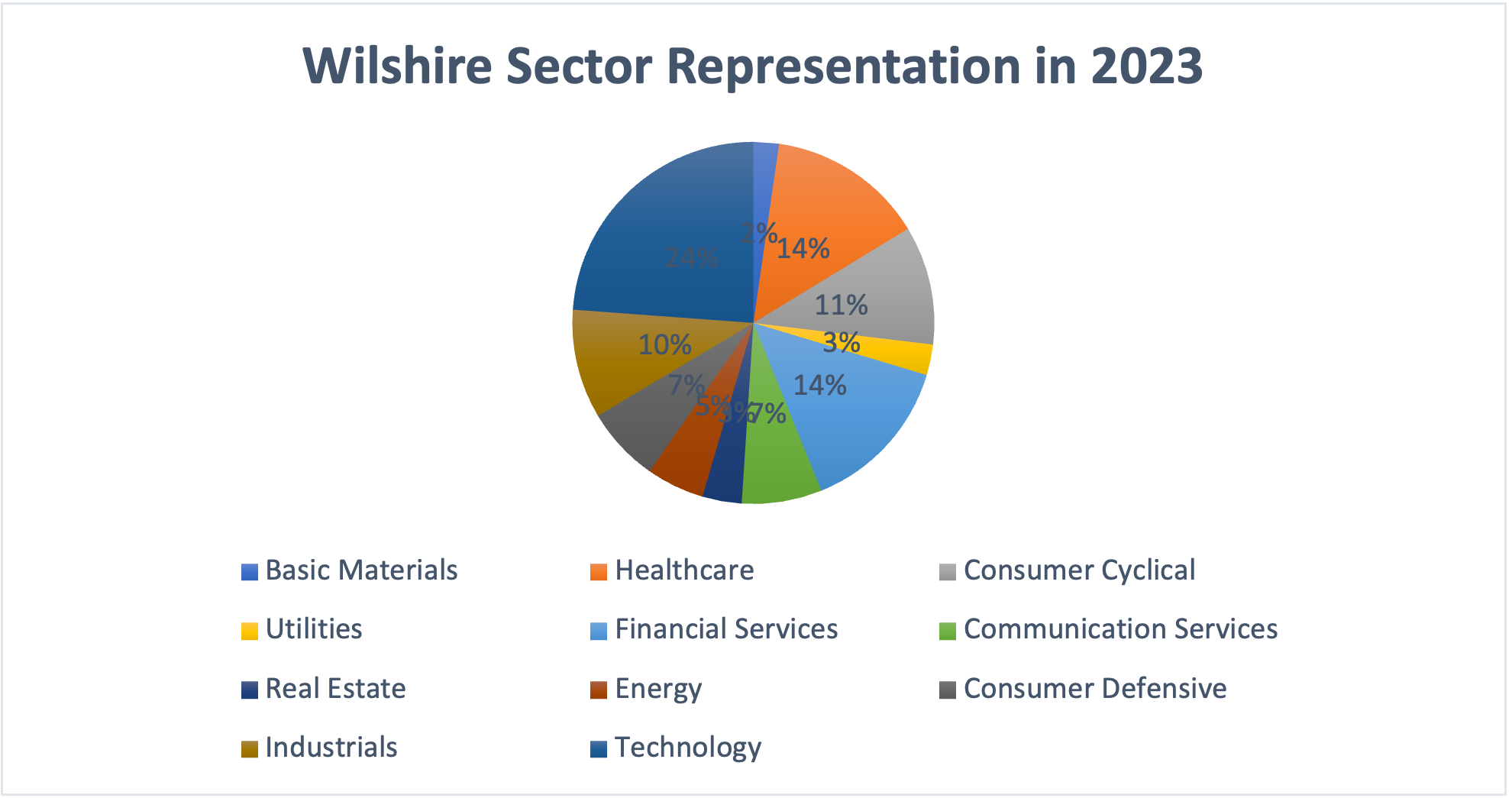
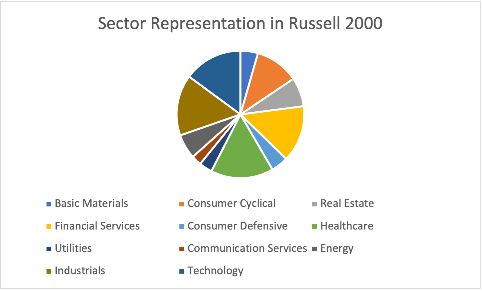
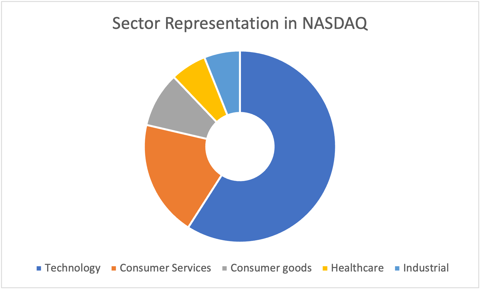
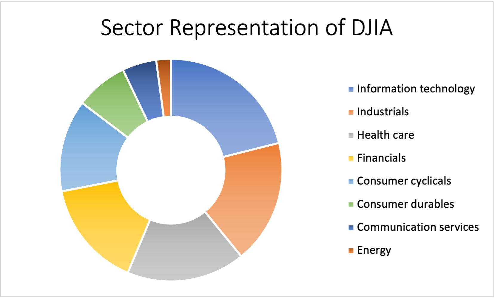
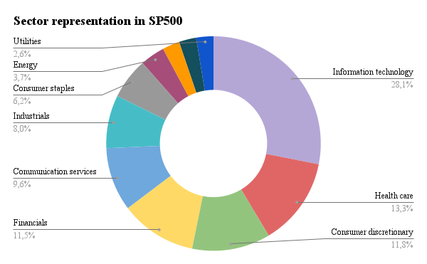
Table 2 below gives the sector representation of the Nikkei 225 index in terms of number of stocks and market capitalization as of January 31, 2023.
Table 2. Sector representation in the Nikkei 225 index.
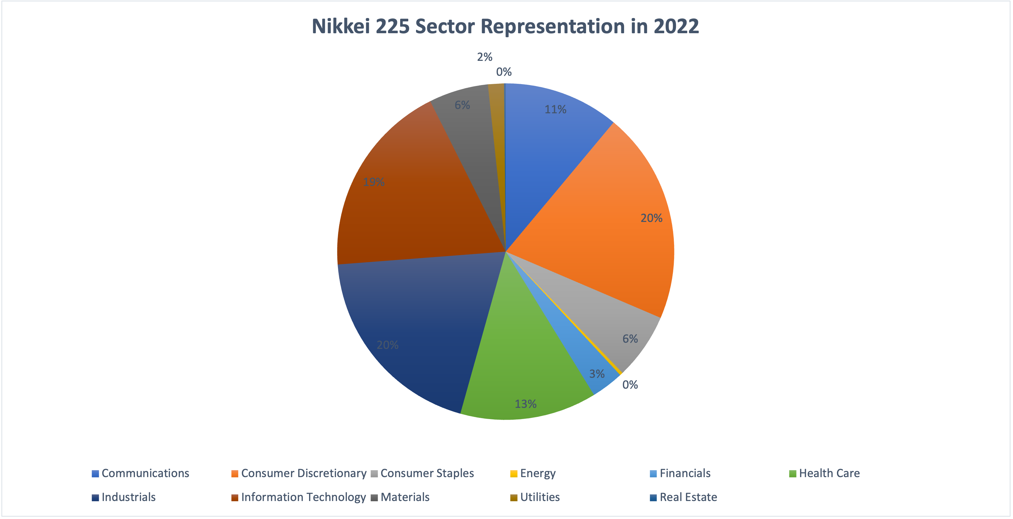
Source: computation by the author (data: YahooFinance! financial website).
Calculation of the Nikkei 225 index value
The Nikkei 225 index is calculated using a price-weighted methodology. This means that the price of each stock in the index is multiplied by the number of shares outstanding to determine the total market value of the company. The Nikkei 225 index is frequently used as a leading indicator of the state of the Japanese stock market, and economy, and as a gauge of trends in the world economy.
The formula to compute the Nikkei 225 is given by
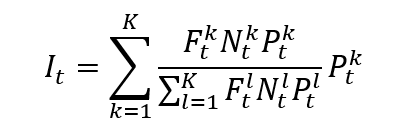
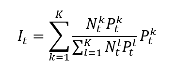
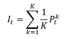
A price-weighted index is calculated by summing the prices of all the assets in the index and dividing by a divisor equal to the number of assets.
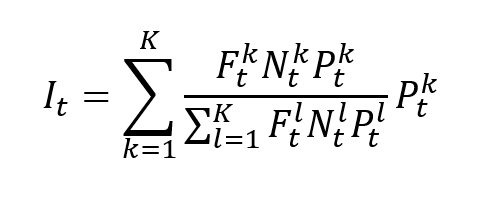
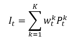
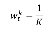
The formula for a price-weighted index is given by
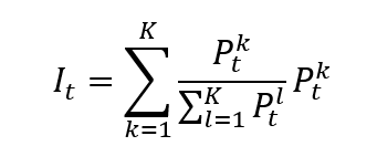
where I is the index value, k a given asset, K the number of assets in the index, Pk the market price of asset k, and t the time of calculation of the index.
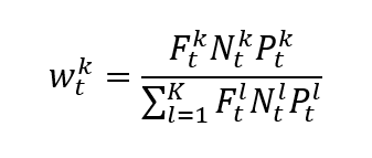
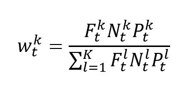
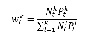
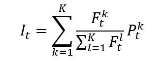
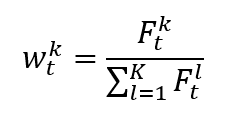
In a price-weighted index, the weight of asset k is given by formula can be rewritten as
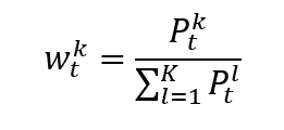
which clearly shows that the weight of each asset in the index is its market price divided by the sum of the market prices of all assets.
Note that the divisor, which is equal to the number of shares, is typically adjusted for events such as stock splits and dividends. The divisor is used to ensure that the value of the index remains consistent over time despite changes in the number of outstanding shares. A more general formula may then be:
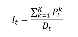
Where D is the divisor which is adjusted over time to account for events such as stock splits and dividends.
Use of the Nikkei 225 index in asset management
Asset managers have shifted their attention in recent years to including environmental, social, and governance (ESG) factors in their investment choices. A number of ESG-related initiatives, such as the development of an ESG index that tracks businesses with high ESG scores, have been introduced by the Nikkei 225 index. The Nikkei 225 index may also be used by asset managers as a component of a more comprehensive global asset allocation strategy. For example, they may use the index to gain exposure to the Asian equity markets while also investing in other regions such as Europe and the Americas. In addition, the Nikkei 225 index can also be used as a risk management tool. Asset managers can spot potential risks and take action to reduce them by comparing a portfolio’s performance to the index.
Benchmark for equity funds
Equity funds that invest in Japanese stocks frequently use the Nikkei 225 index as a benchmark. The index is used by investment managers and individual investors to assess and contrast the performance of their holdings of Japanese equities with the performance of the overall market. Japanese exchange-traded funds (ETFs) and other investment products that follow the Japanese equity market use the index as a benchmark as well. Additionally, derivatives like futures and options that enable investors to trade on the Japanese equity market are based on the Nikkei 225 index.
Financial products around the Nikkei 225 index
There are several financial products that track the performance of the Nikkei 225 index, allowing investors to gain exposure to the Japanese stock market.
- Nikkei 225 ETFs are a popular way for investors to gain exposure to the Japanese equity market, as they offer a low-cost and convenient way to invest in a diversified basket of stocks. Some of the largest Nikkei 225 ETFs by assets under management include the iShares Nikkei 225 ETF (NKY), the Nomura Nikkei 225 ETF (1321), and the Daiwa ETF Nikkei 225 (1320).
- There are also mutual funds and index funds that track the Nikkei 225 index. These funds typically have higher fees than ETFs but may offer different investment strategies or options for investors.
- Certificates are structured products that allow investors to gain exposure to the Nikkei 225 index without actually owning the underlying assets.
- Futures contracts based on the Nikkei 225 index are also available for investors who want to trade the index with leverage or for hedging purposes. These futures contracts trade on the Osaka Exchange, a subsidiary of the Japan Exchange Group.
Historical data for the Nikkei 225 index
How to get the data?
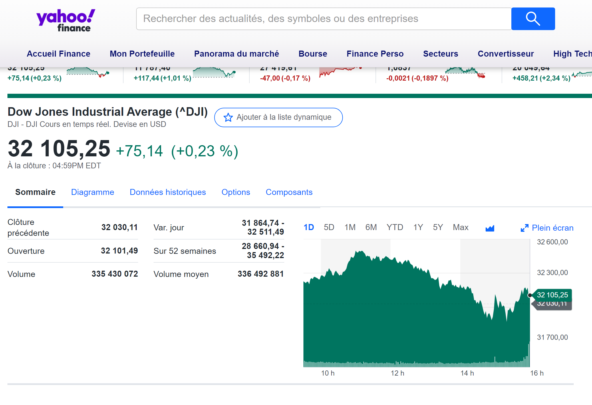
The Nikkei 225 index is the most common index used in finance, and historical data for the Nikkei 225 index can be easily downloaded from the internet.
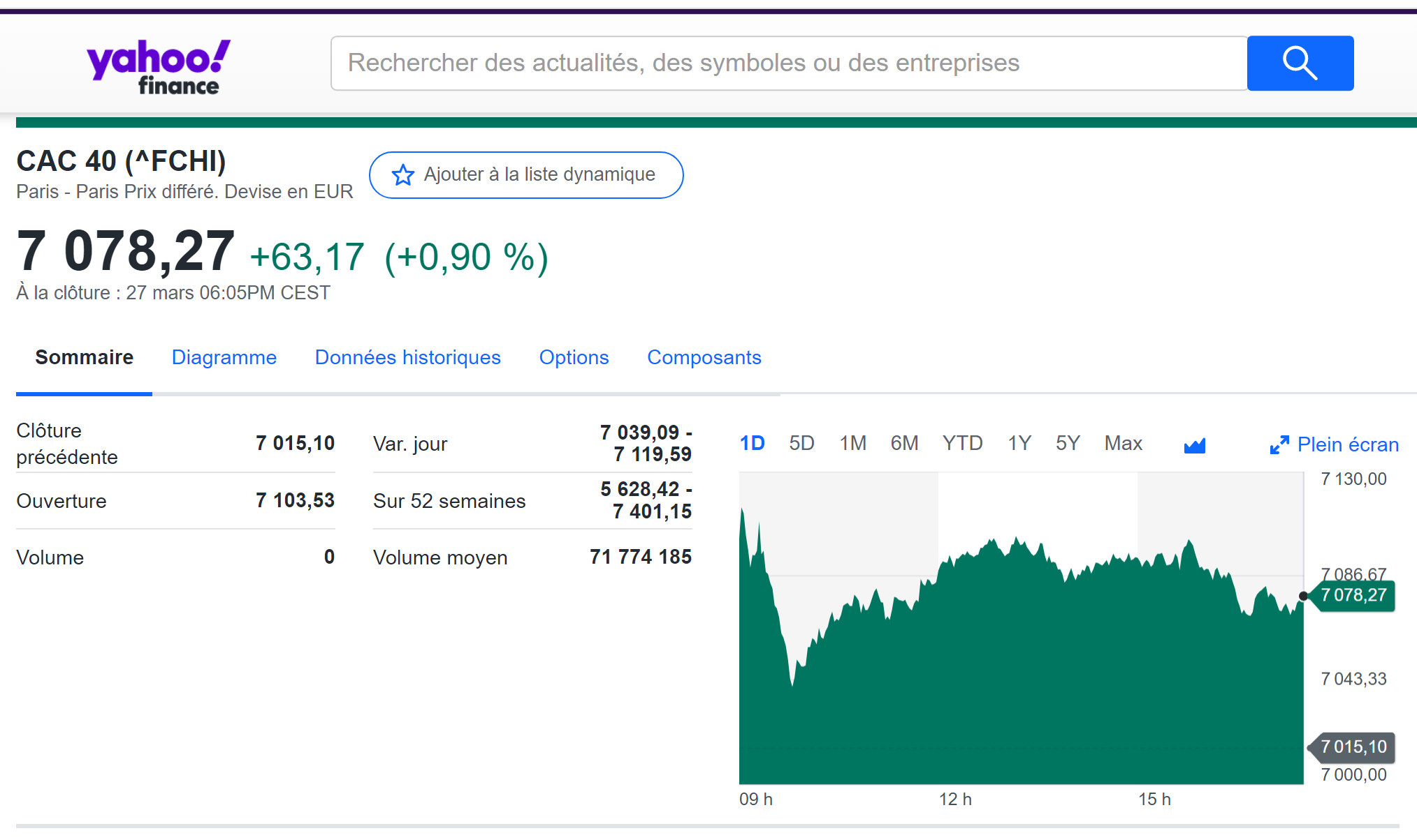
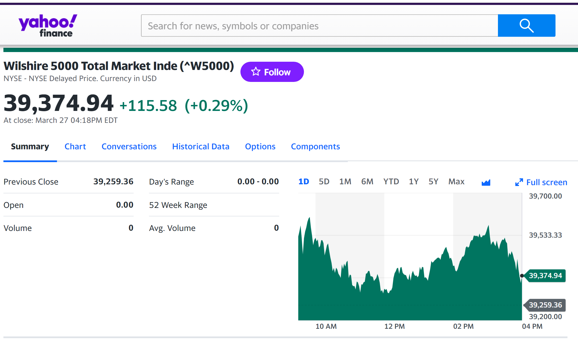
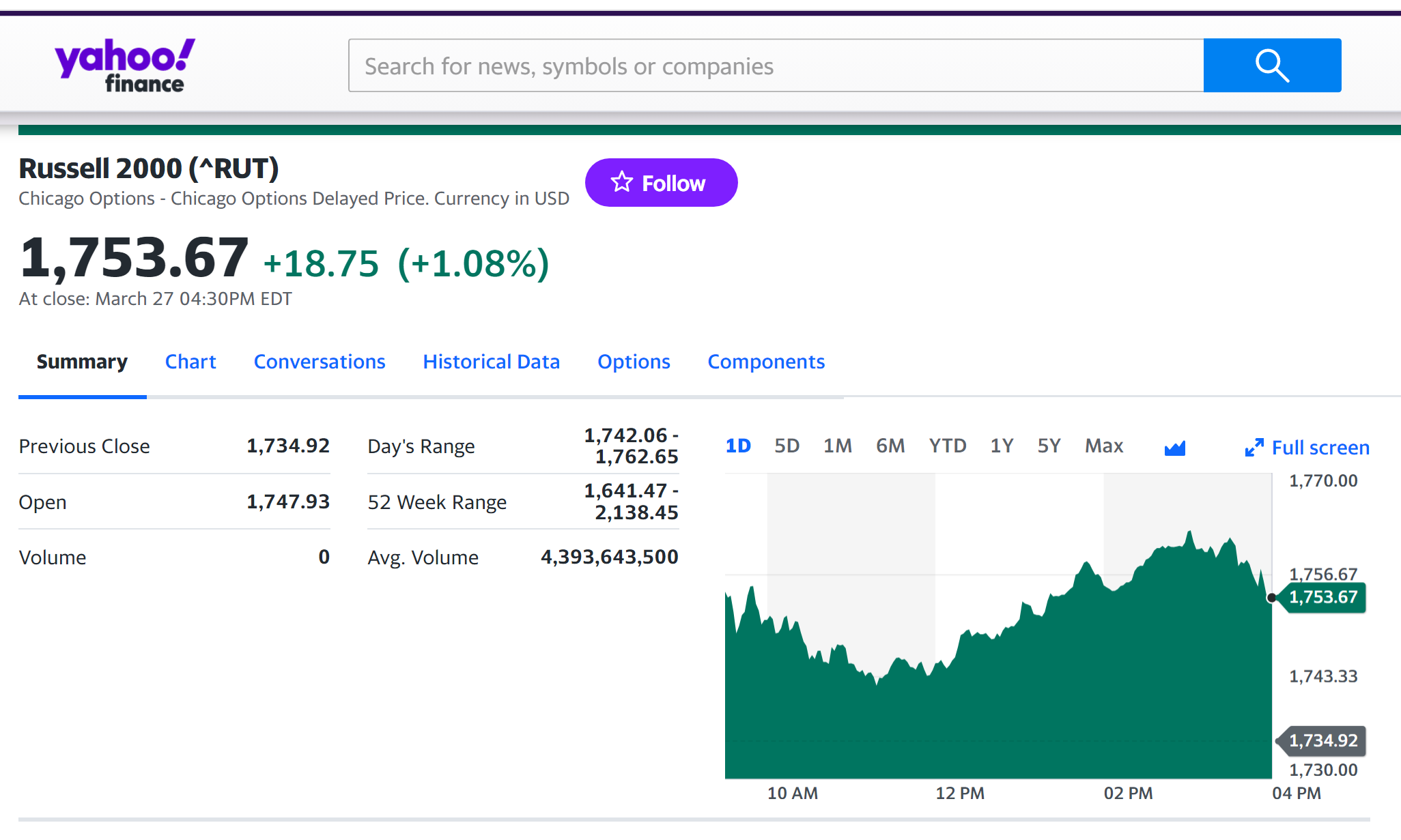
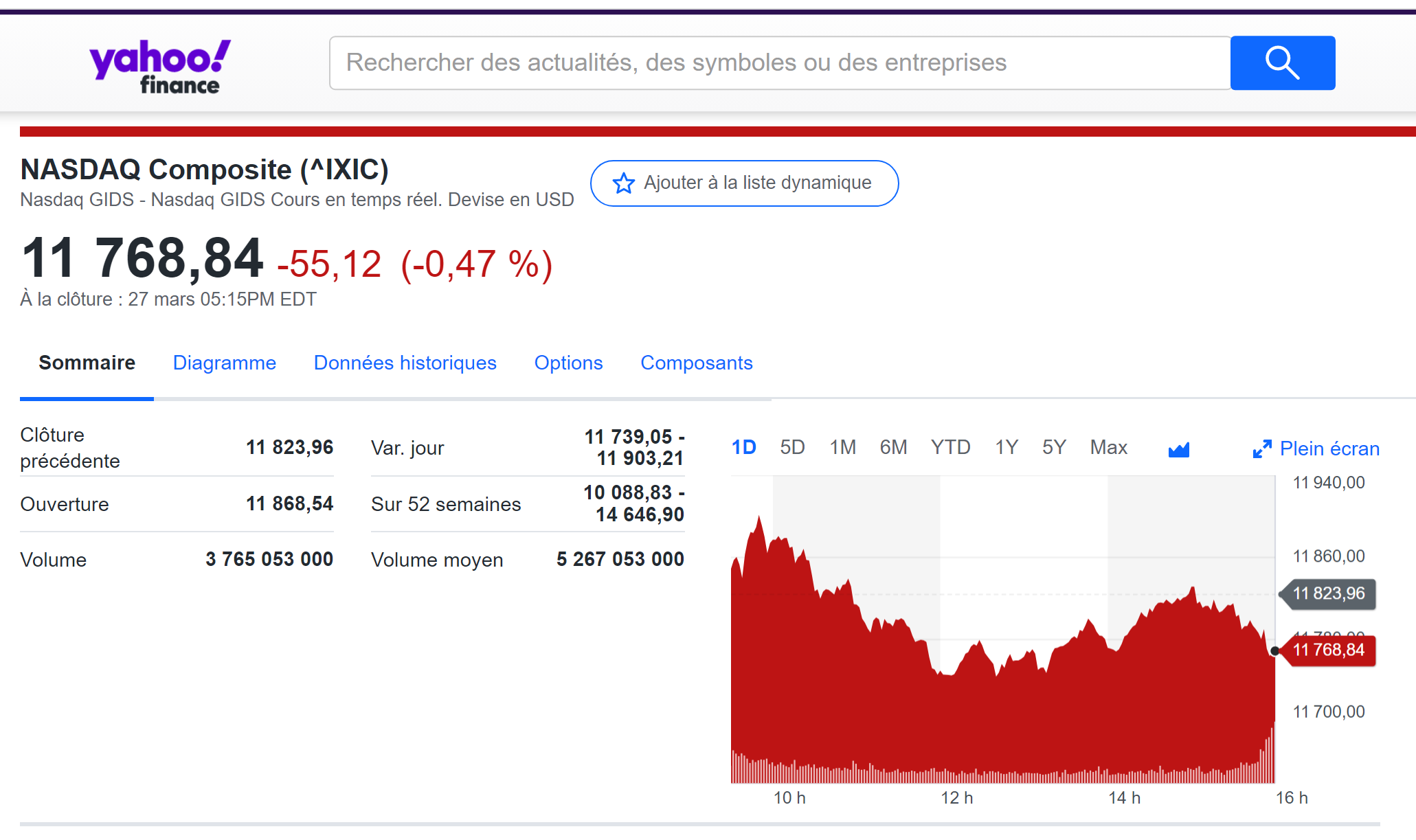
For example, you can download data for the Nikkei 225 index from March 1, 1990 on Yahoo! Finance (the Yahoo! code for Nikkei 225 index is ^N225).
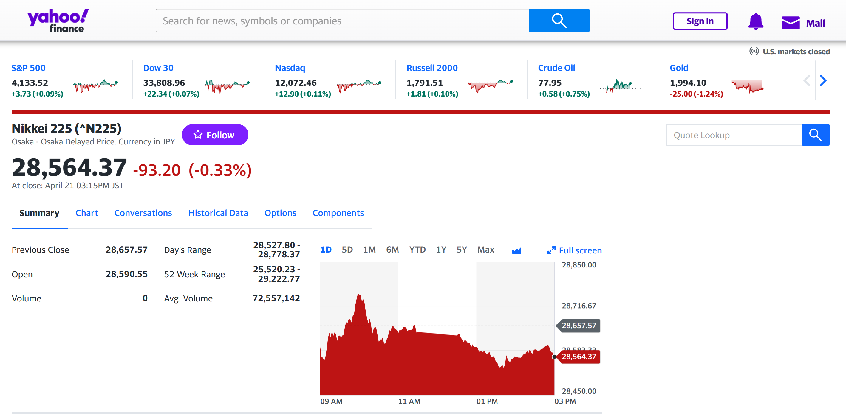
Source: Yahoo! Finance.
You can also download the same data from a Bloomberg terminal.
R program
The R program below written by Shengyu ZHENG allows you to download the data from Yahoo! Finance website and to compute summary statistics and risk measures about the Nikkei 225 index.

Data file
The R program that you can download above allows you to download the data for the Nikkei 225 index from the Yahoo! Finance website. The database starts on March 1, 1990. It also computes the returns (logarithmic returns) from closing prices.
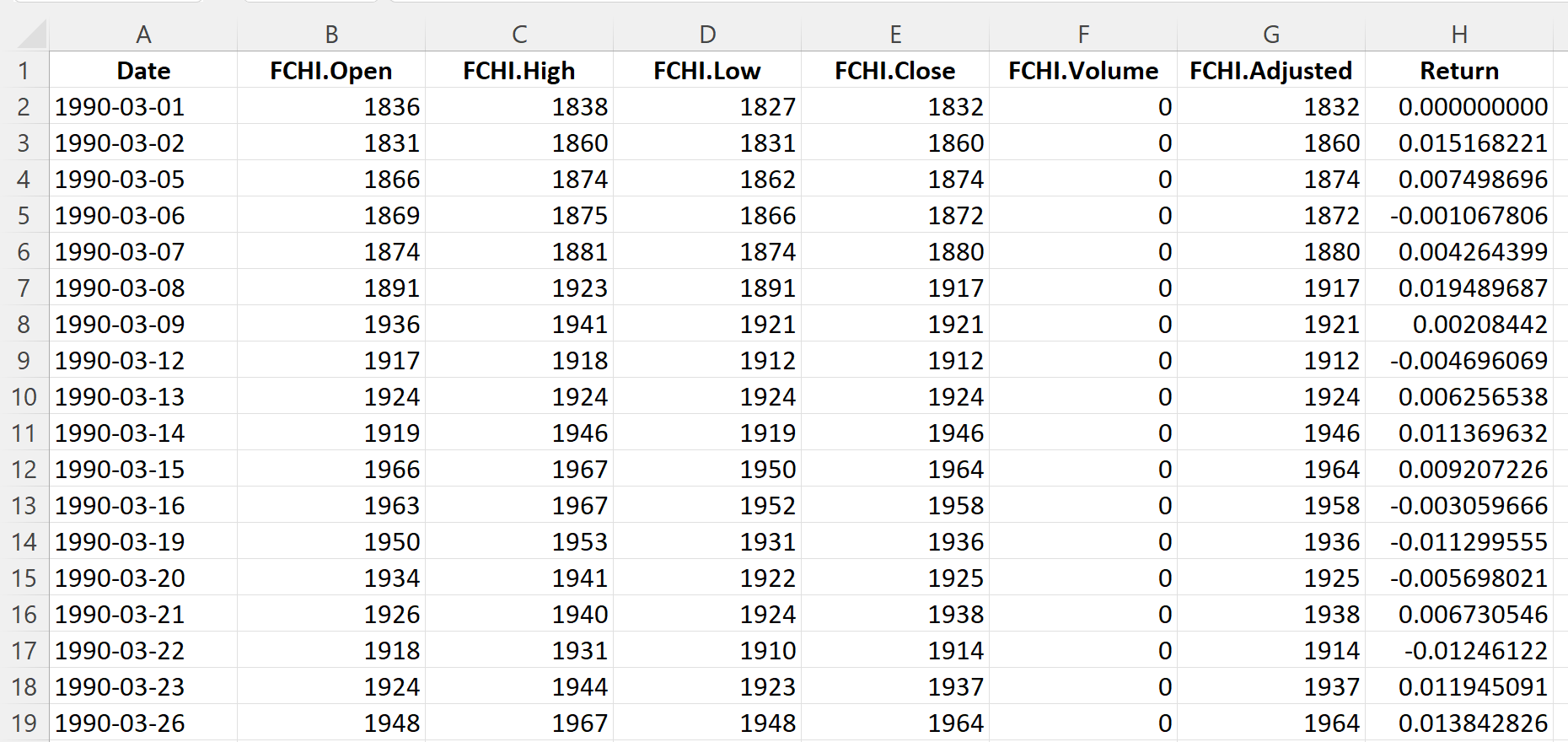
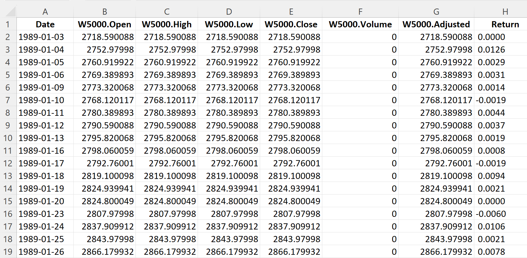
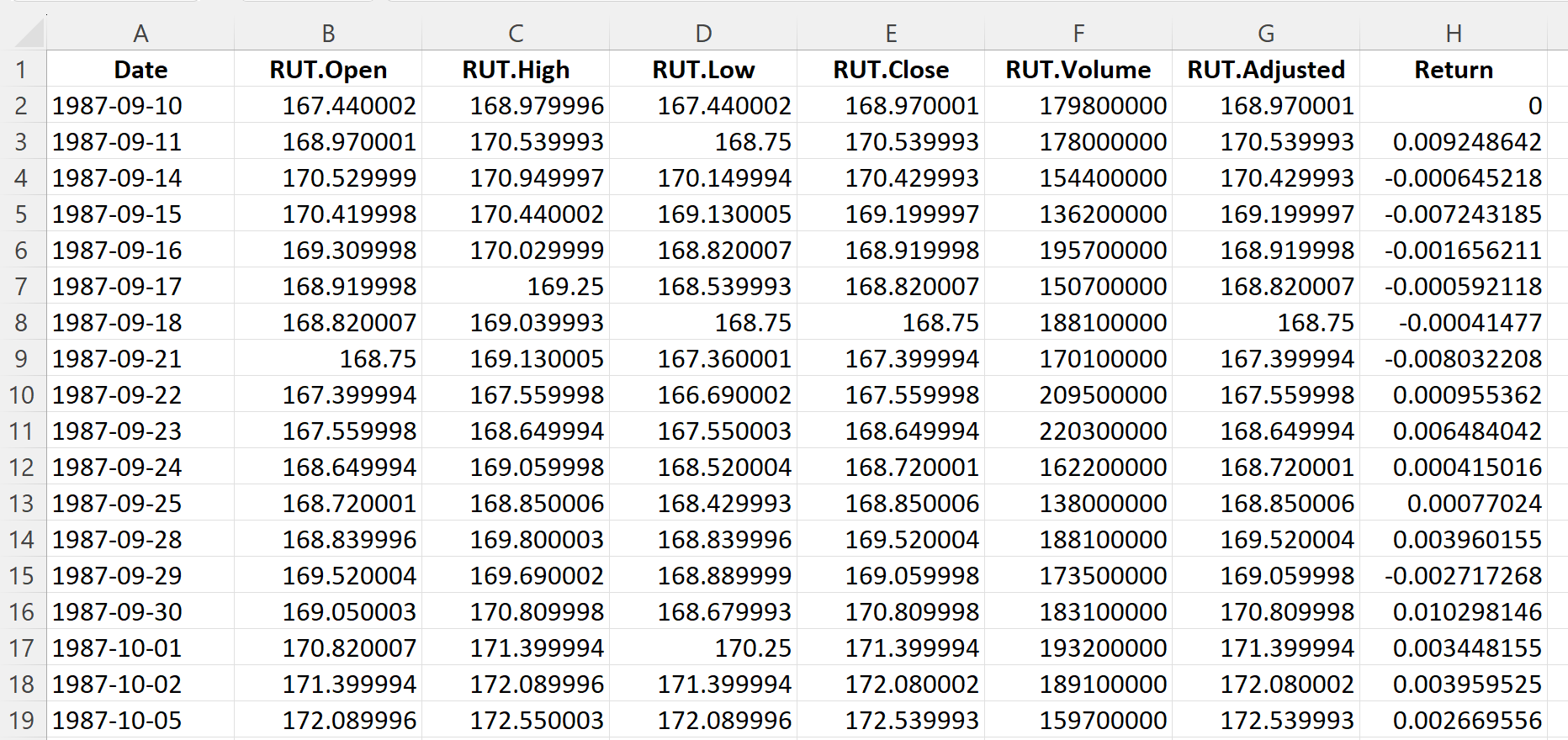
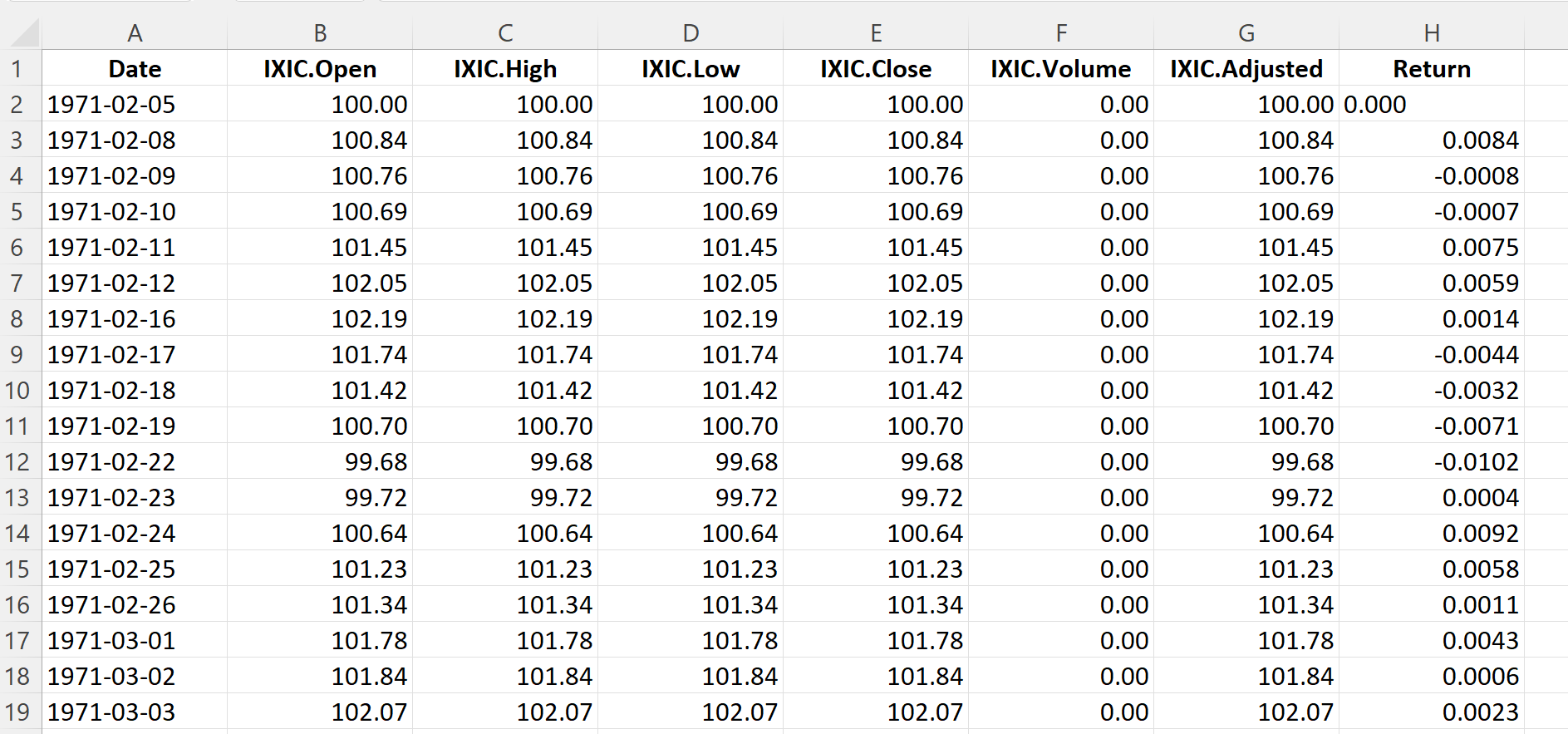
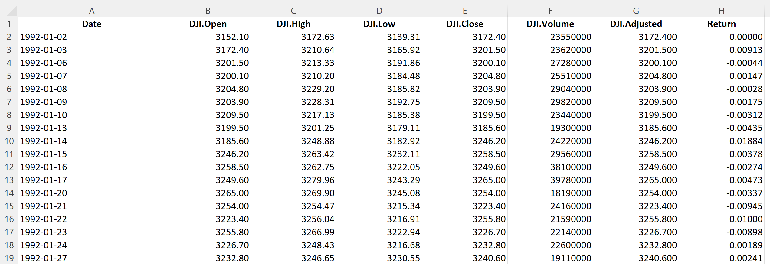
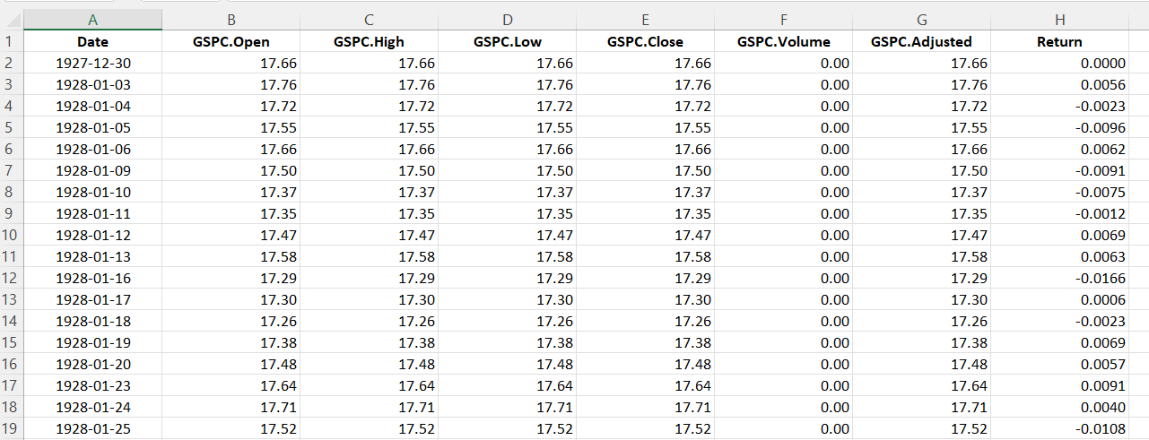
Table 3 below represents the top of the data file for the Nikkei 225 index downloaded from the Yahoo! Finance website with the R program.
Table 3. Top of the data file for the Nikkei 225 index.
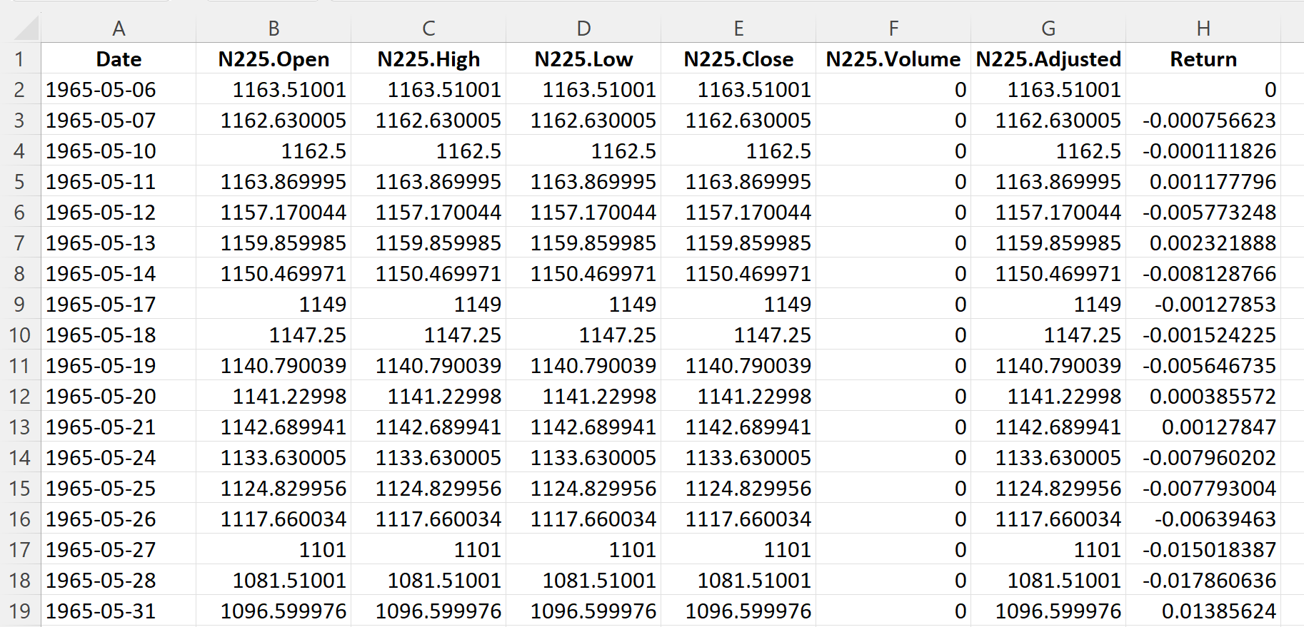
Source: computation by the author (data: Yahoo! Finance website).
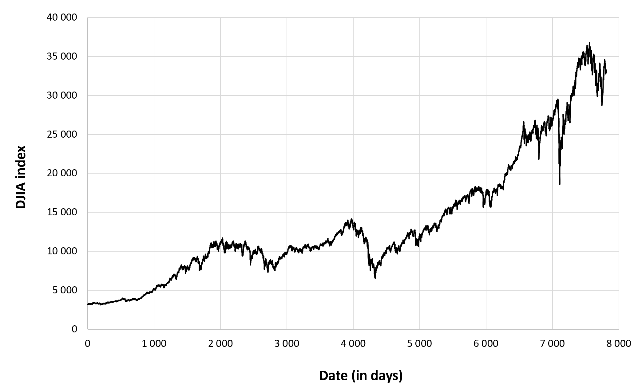
Evolution of the Nikkei 225 index
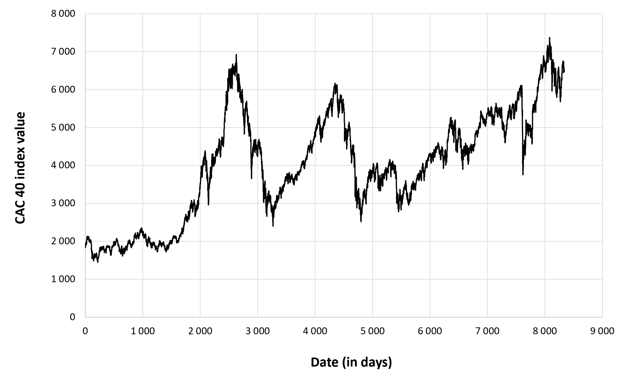
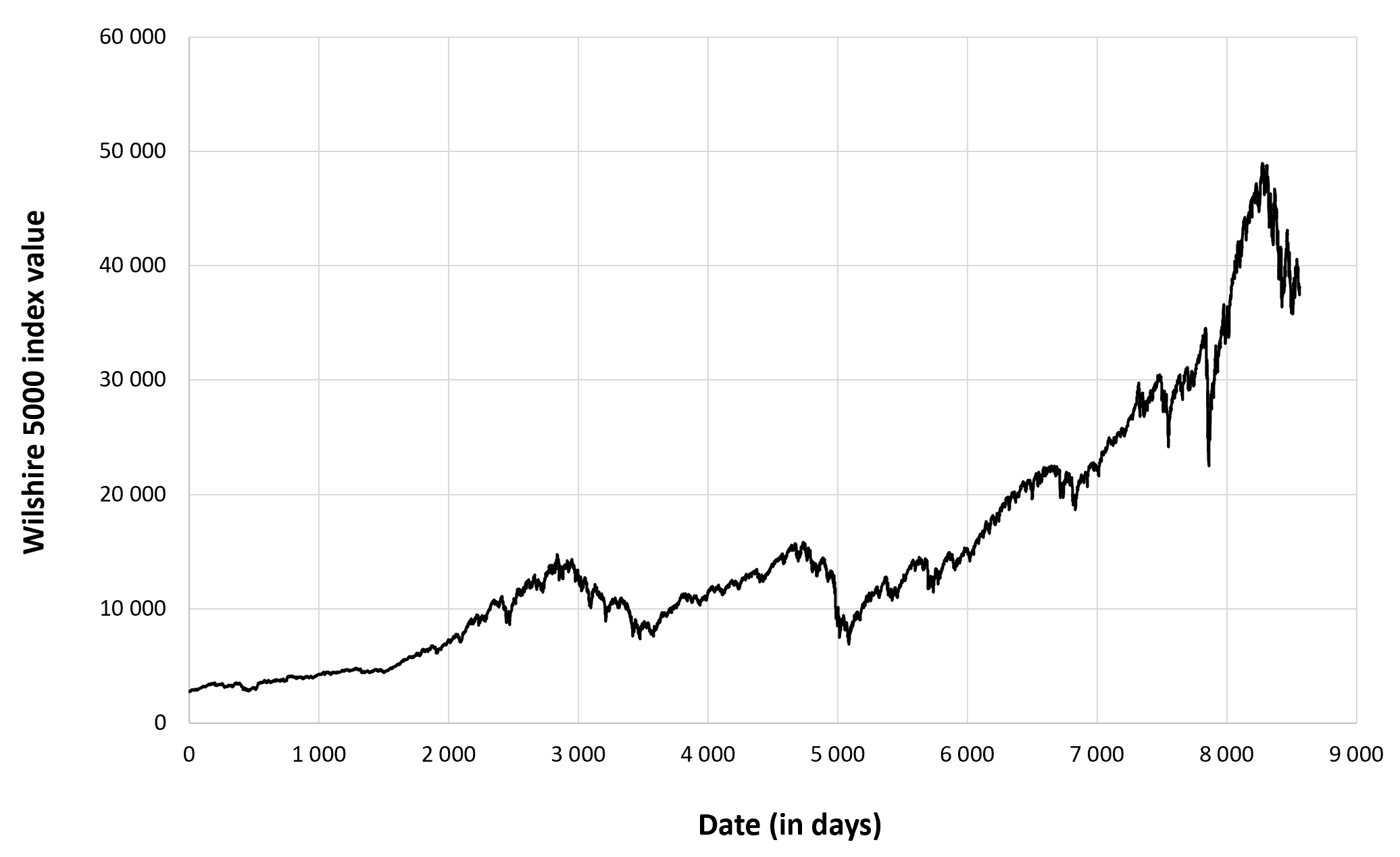
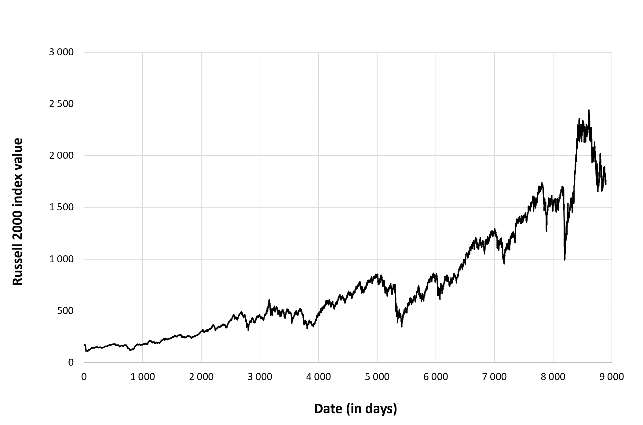
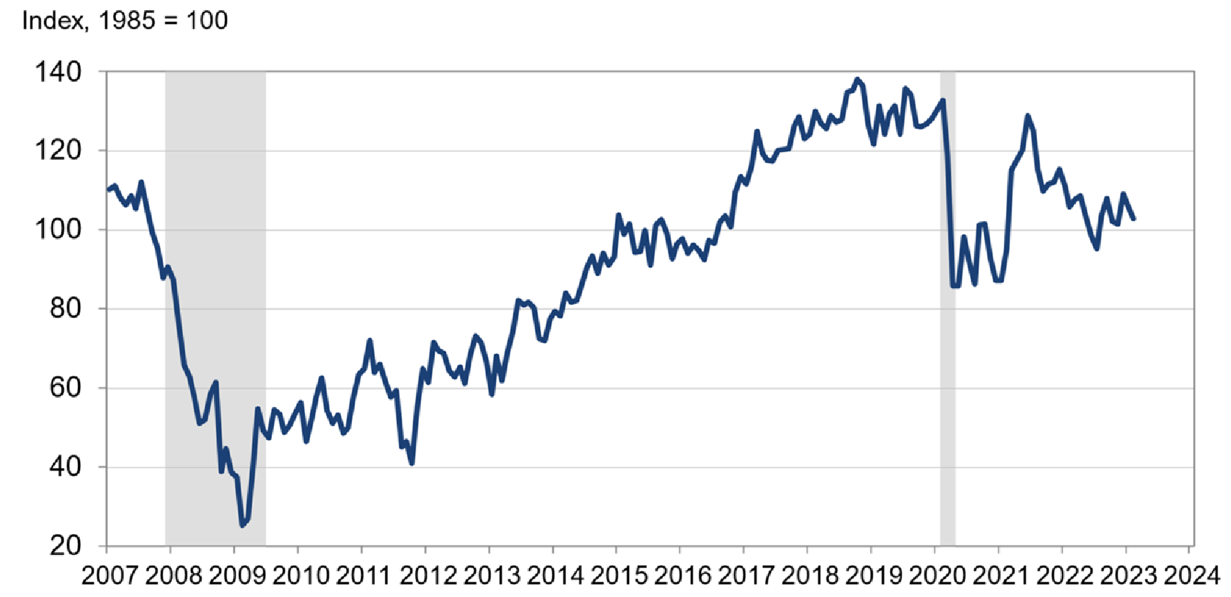
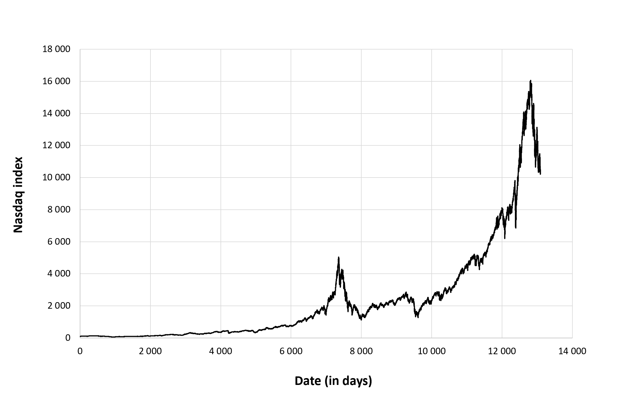
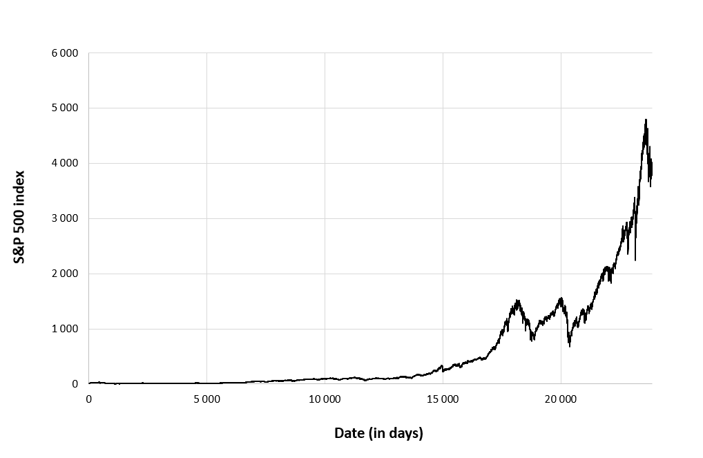
Figure 1 below gives the evolution of the Nikkei 225 index from March 1, 1990 to December 30, 2022 on a daily basis.
Figure 1. Evolution of the Nikkei 225 index.
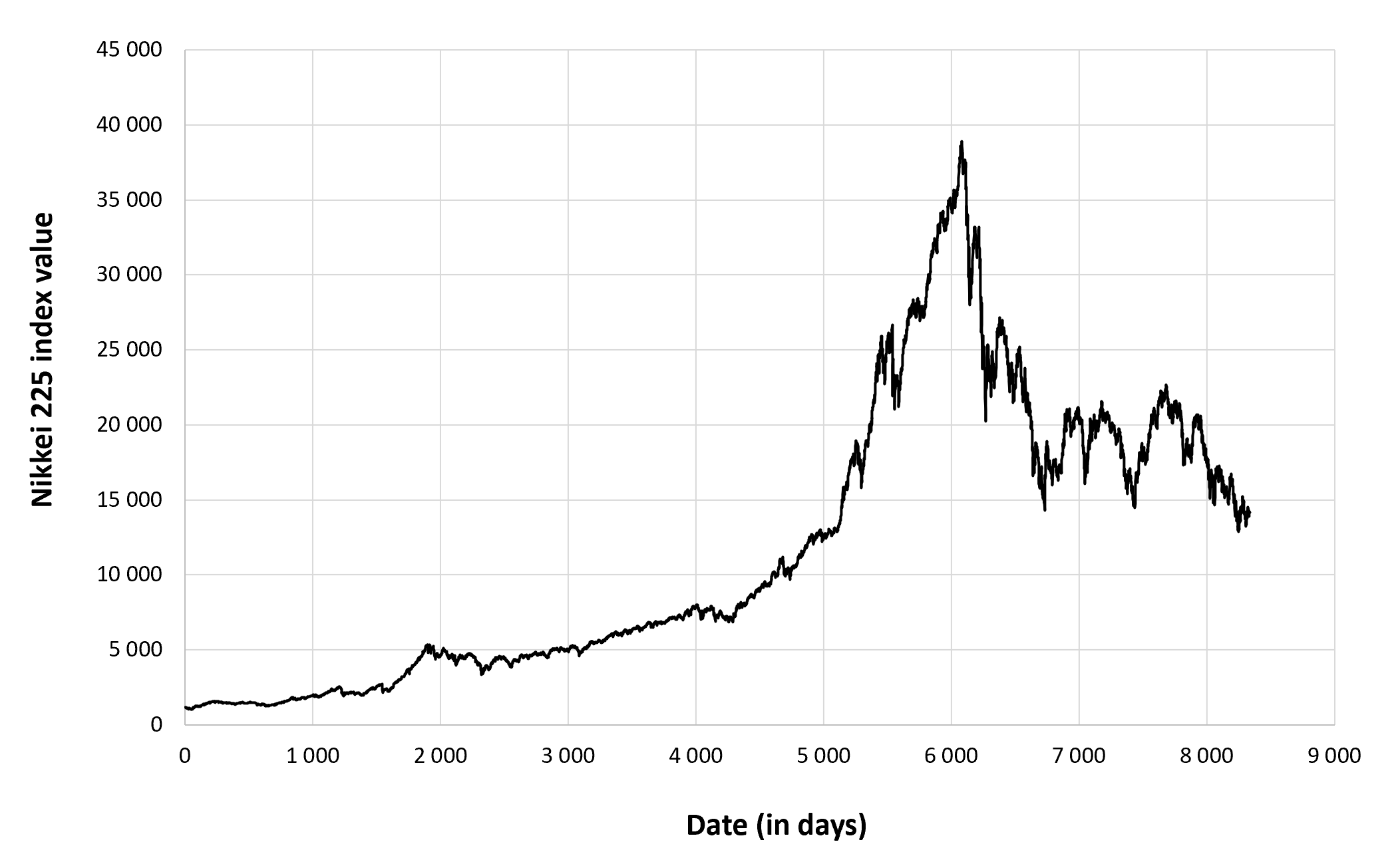
Source: computation by the author (data: Yahoo! Finance website).
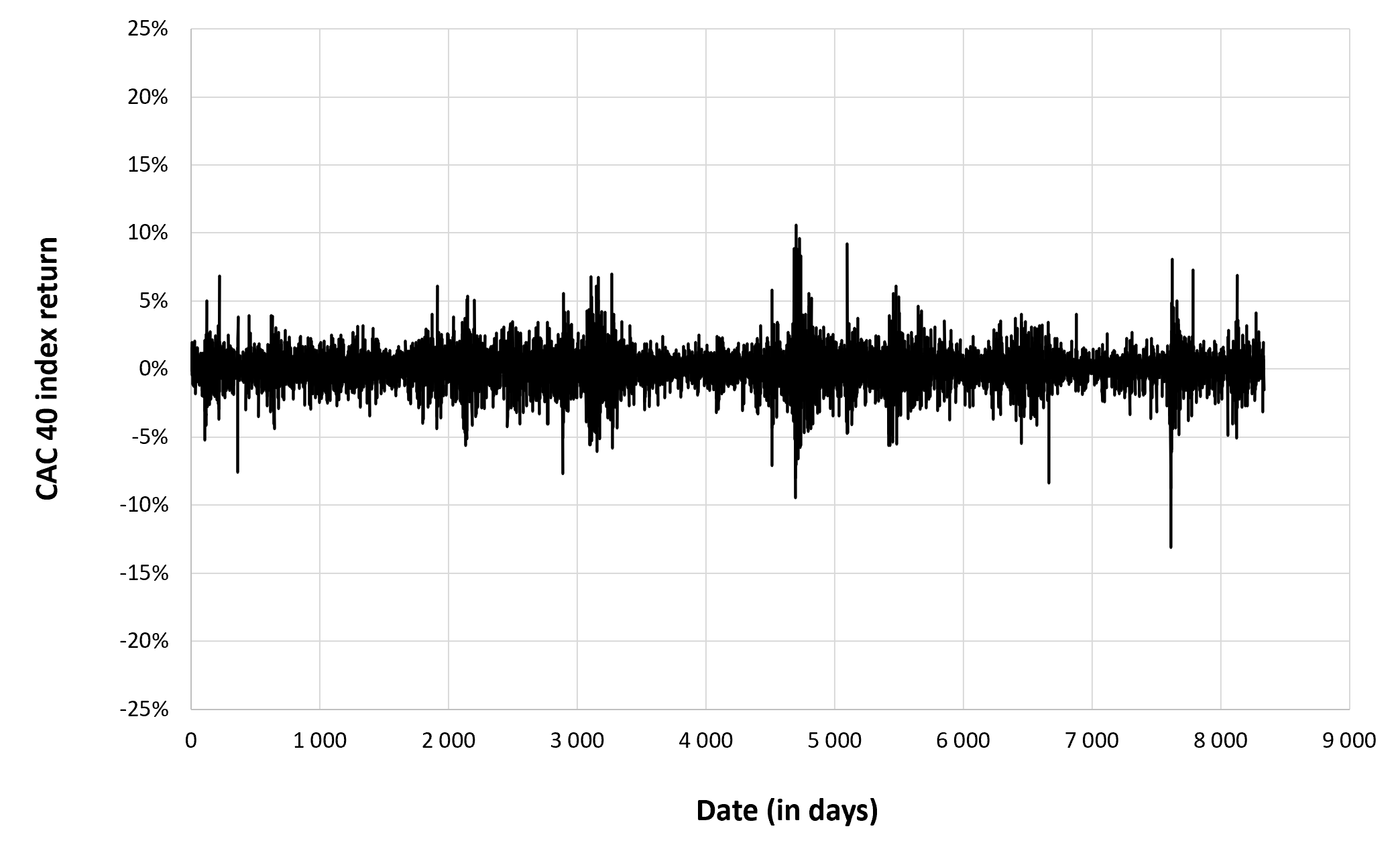
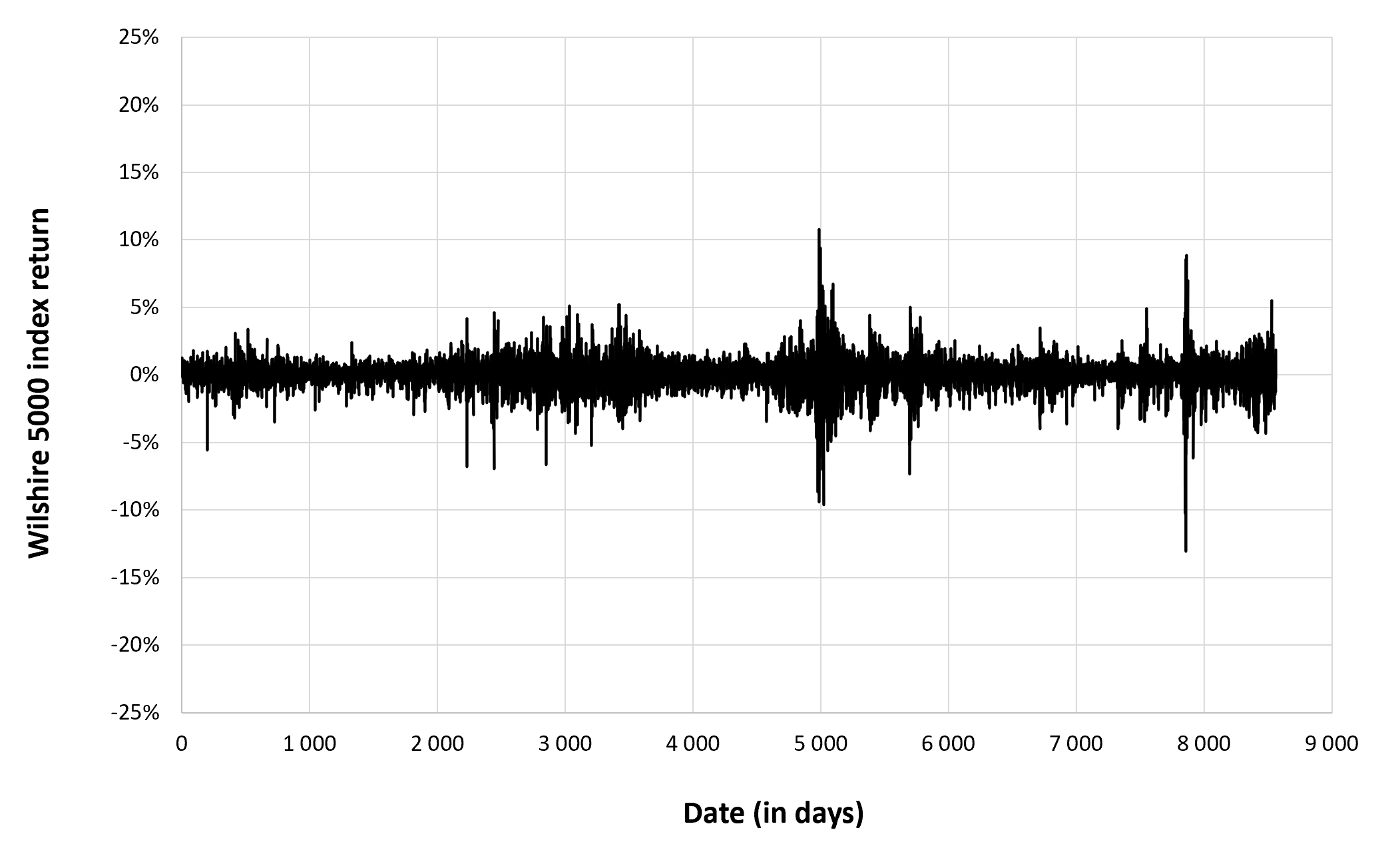
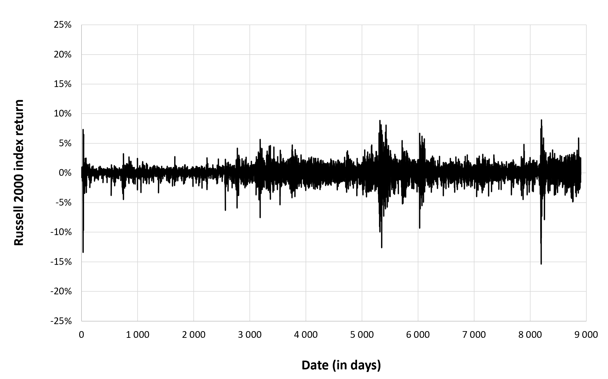
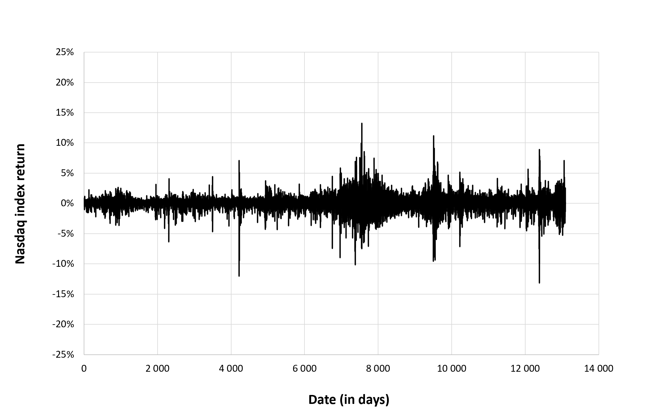
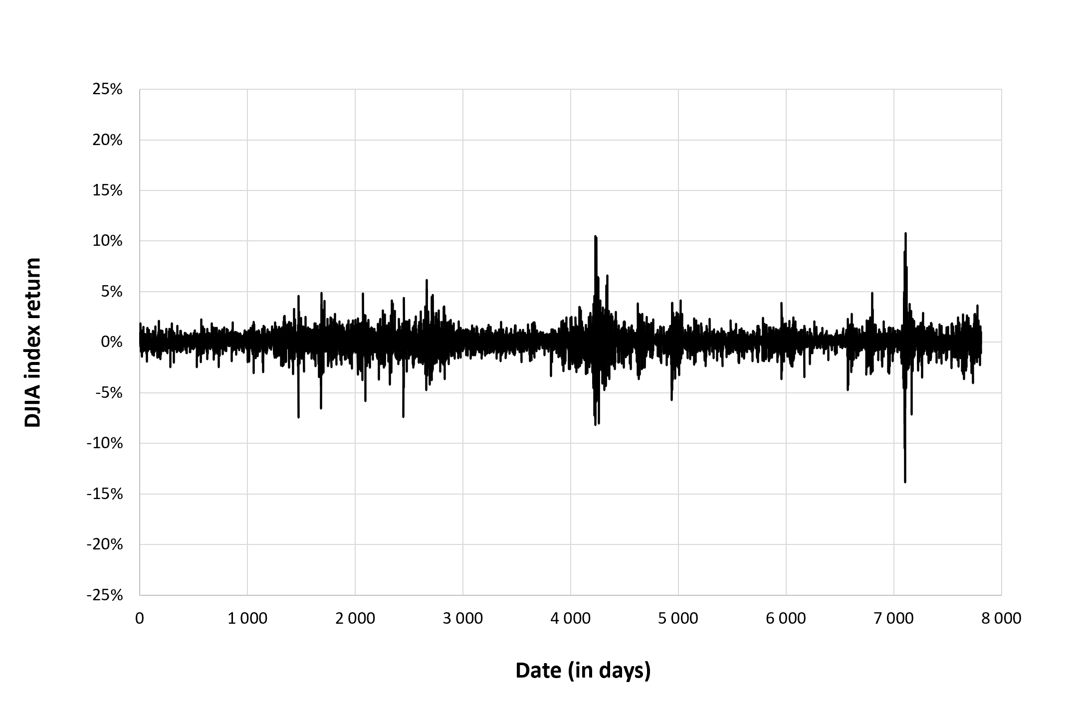
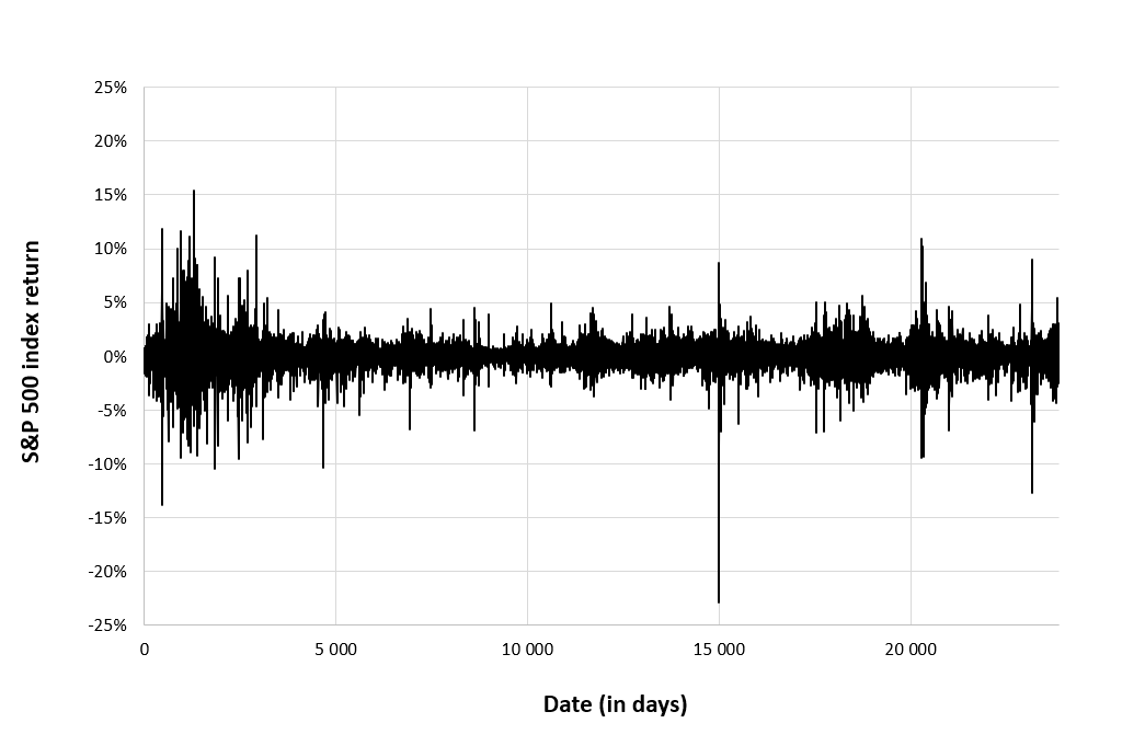
Figure 2 below gives the evolution of the Nikkei 225 index returns from March 1, 1990 to December 30, 2022 on a daily basis.
Figure 2. Evolution of the Nikkei 225 index returns.
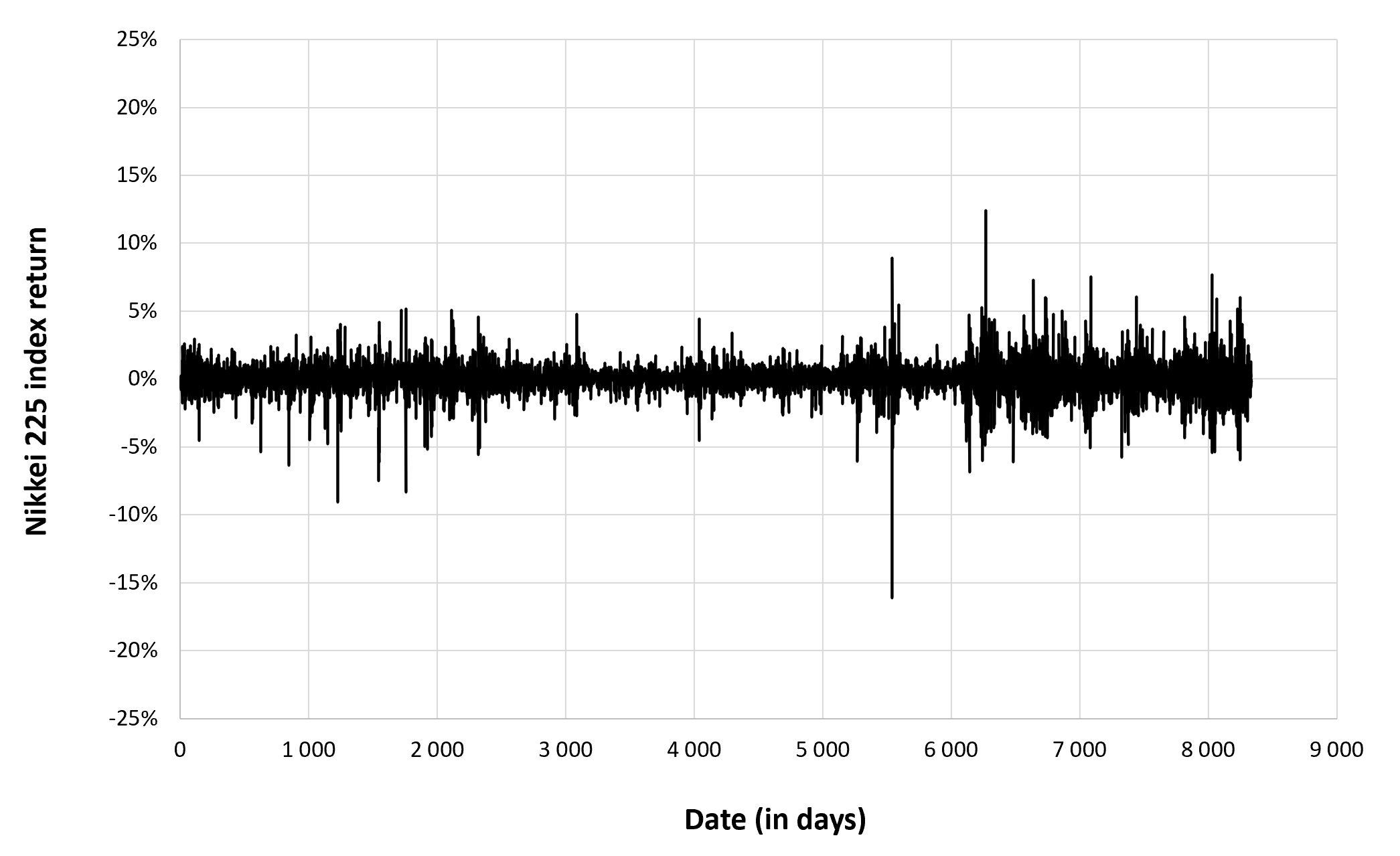
Source: computation by the author (data: Yahoo! Finance website).
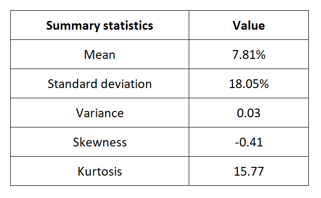
Summary statistics for the Nikkei 225 index
The R program that you can download above also allows you to compute summary statistics about the returns of the Nikkei 225 index.
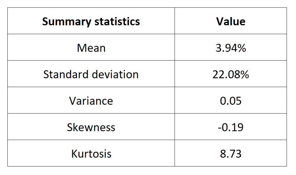
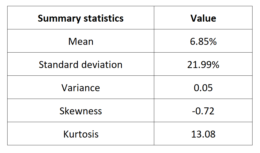
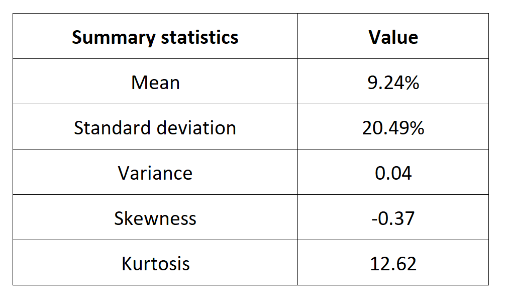
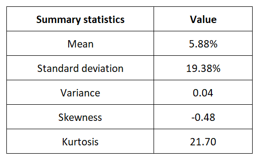
Table 4 below presents the following summary statistics estimated for the Nikkei 225 index:
- The mean
- The standard deviation (the squared root of the variance)
- The skewness
- The kurtosis.
The mean, the standard deviation / variance, the skewness, and the kurtosis refer to the first, second, third and fourth moments of statistical distribution of returns respectively.
Table 4. Summary statistics for the Nikkei 225 index.
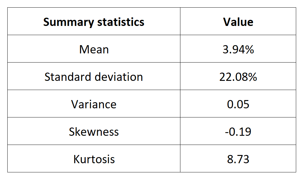
Source: computation by the author (data: Yahoo! Finance website).
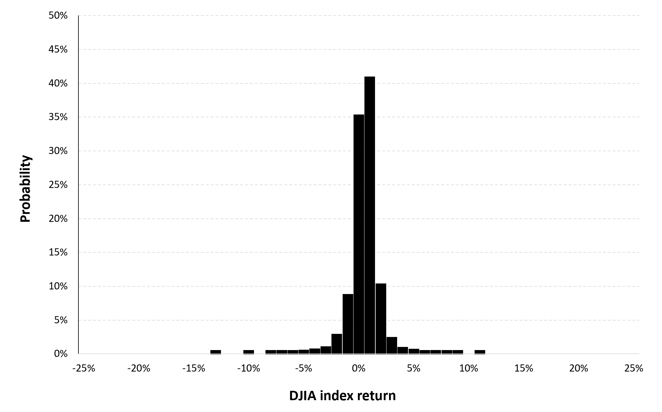
Statistical distribution of the Nikkei 225 index returns
Historical distribution
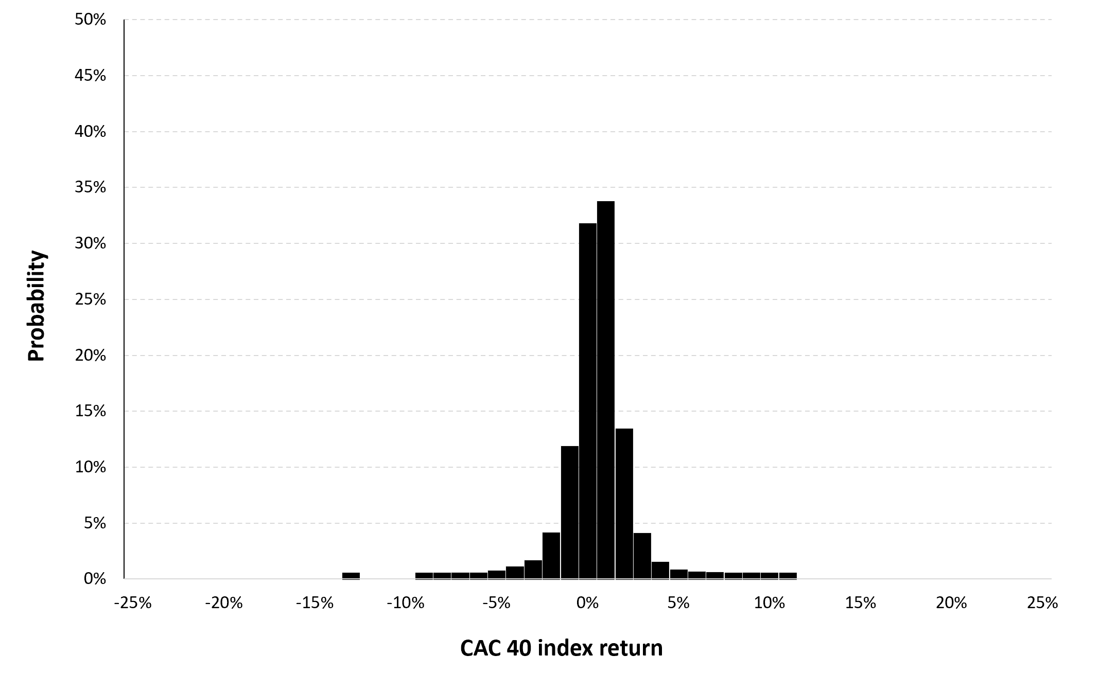
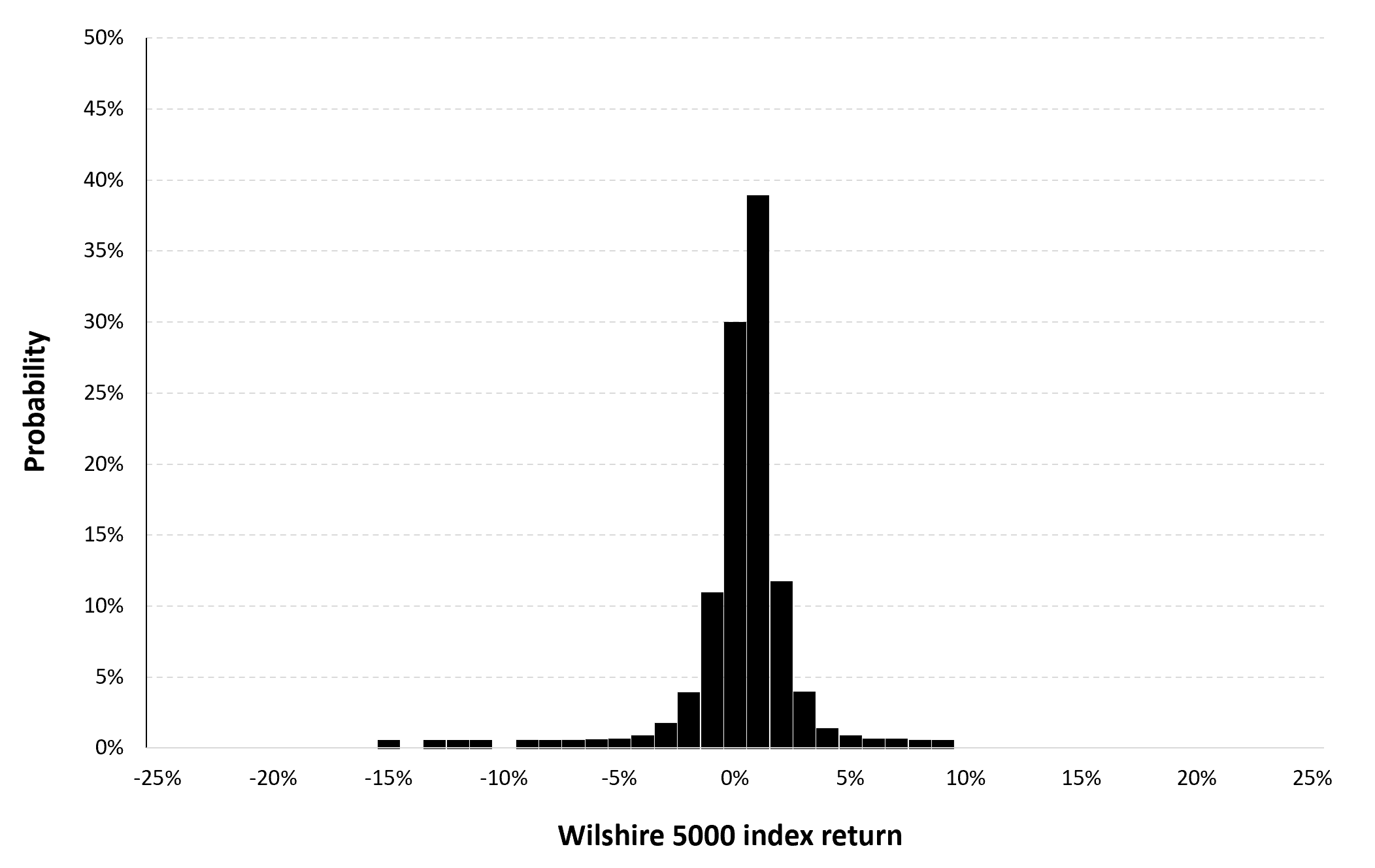
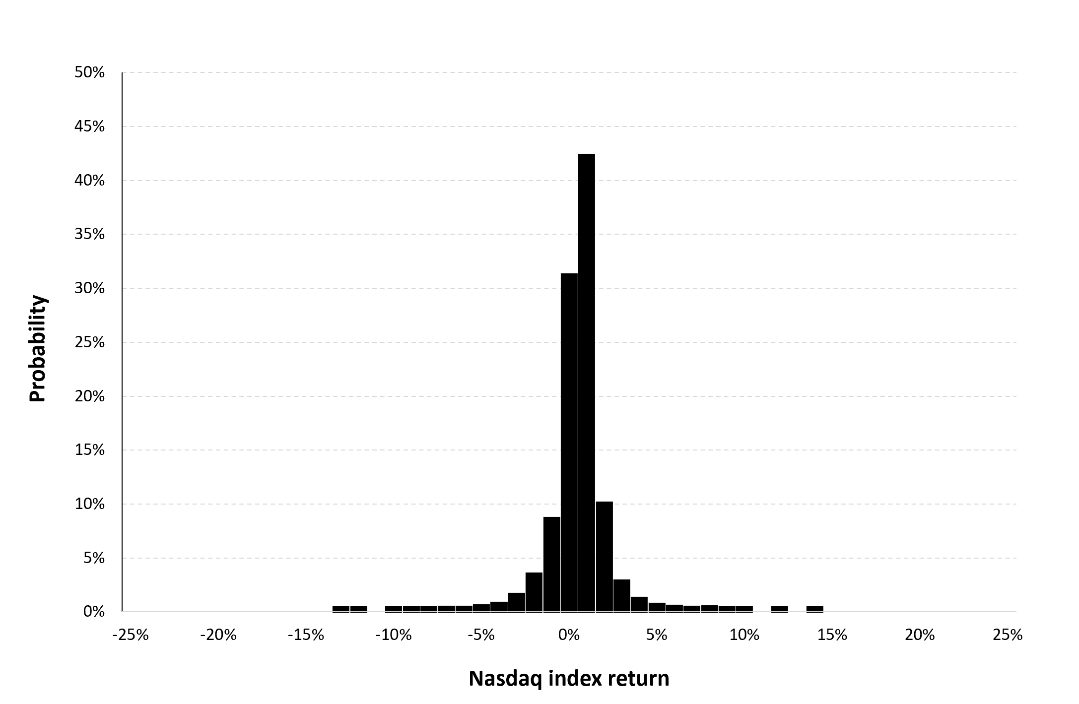
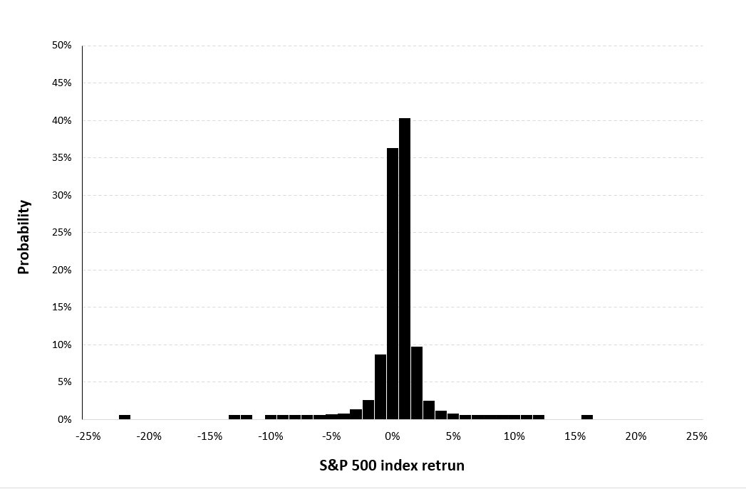
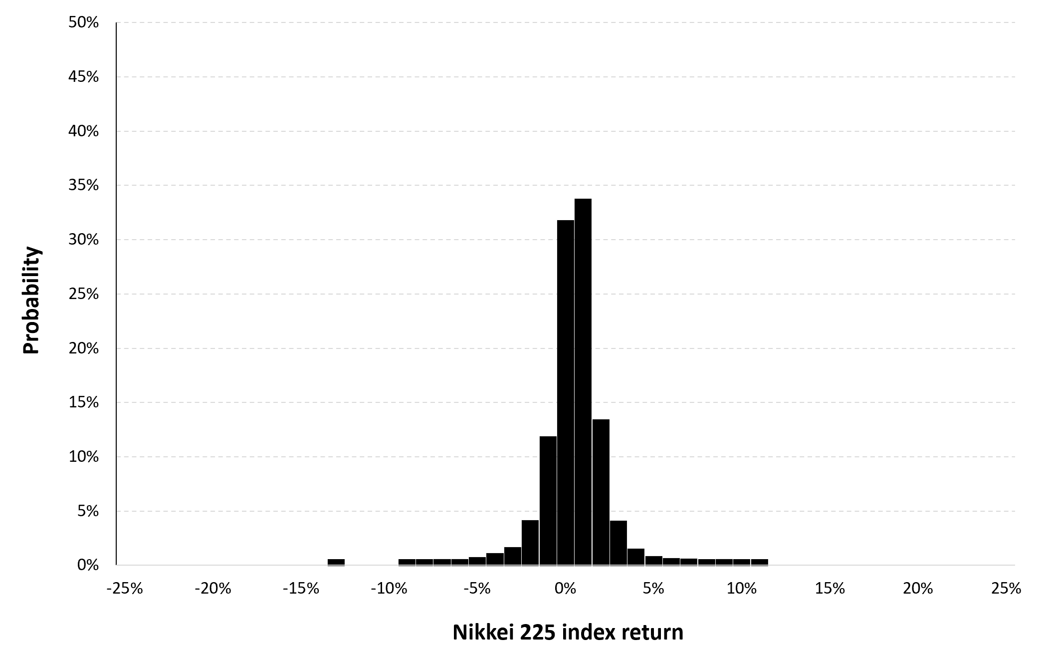
Figure 3 represents the historical distribution of the Nikkei 225 index daily returns for the period from March 1, 1990 to December 30, 2022.
Figure 3. Historical distribution of the Nikkei 225 index returns.
Source: computation by the author (data: Yahoo! Finance website).
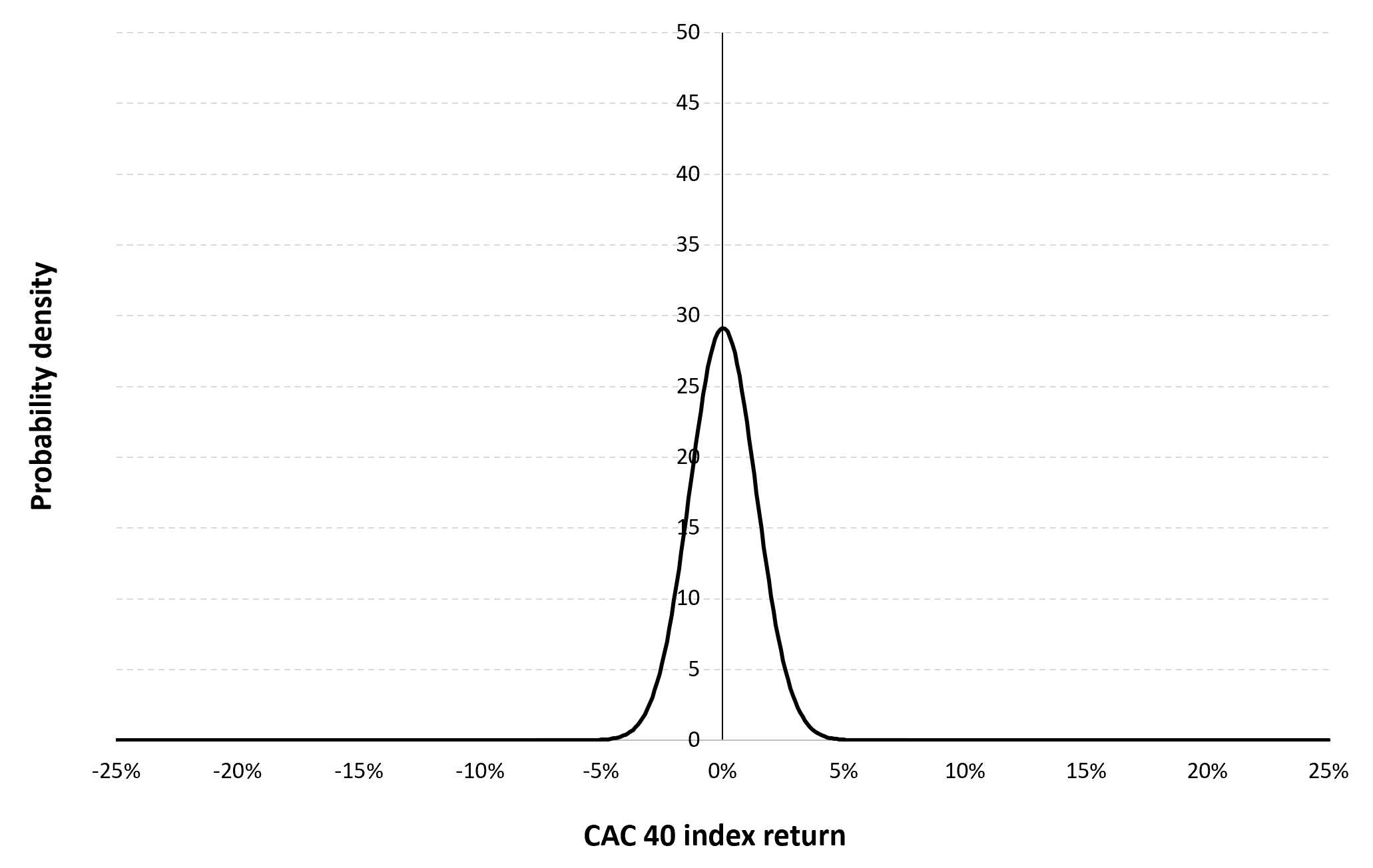
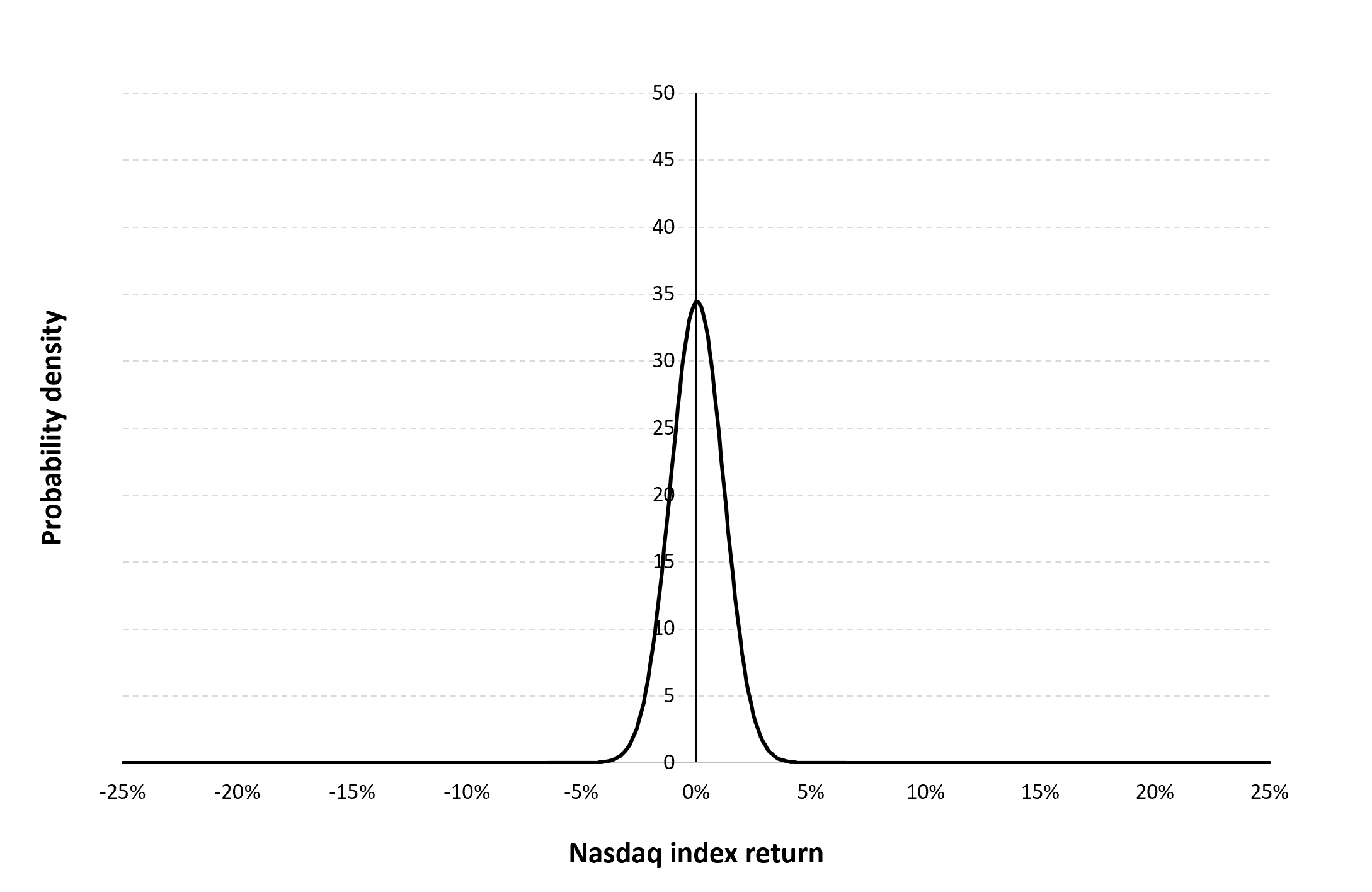
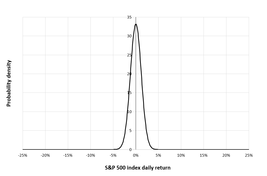
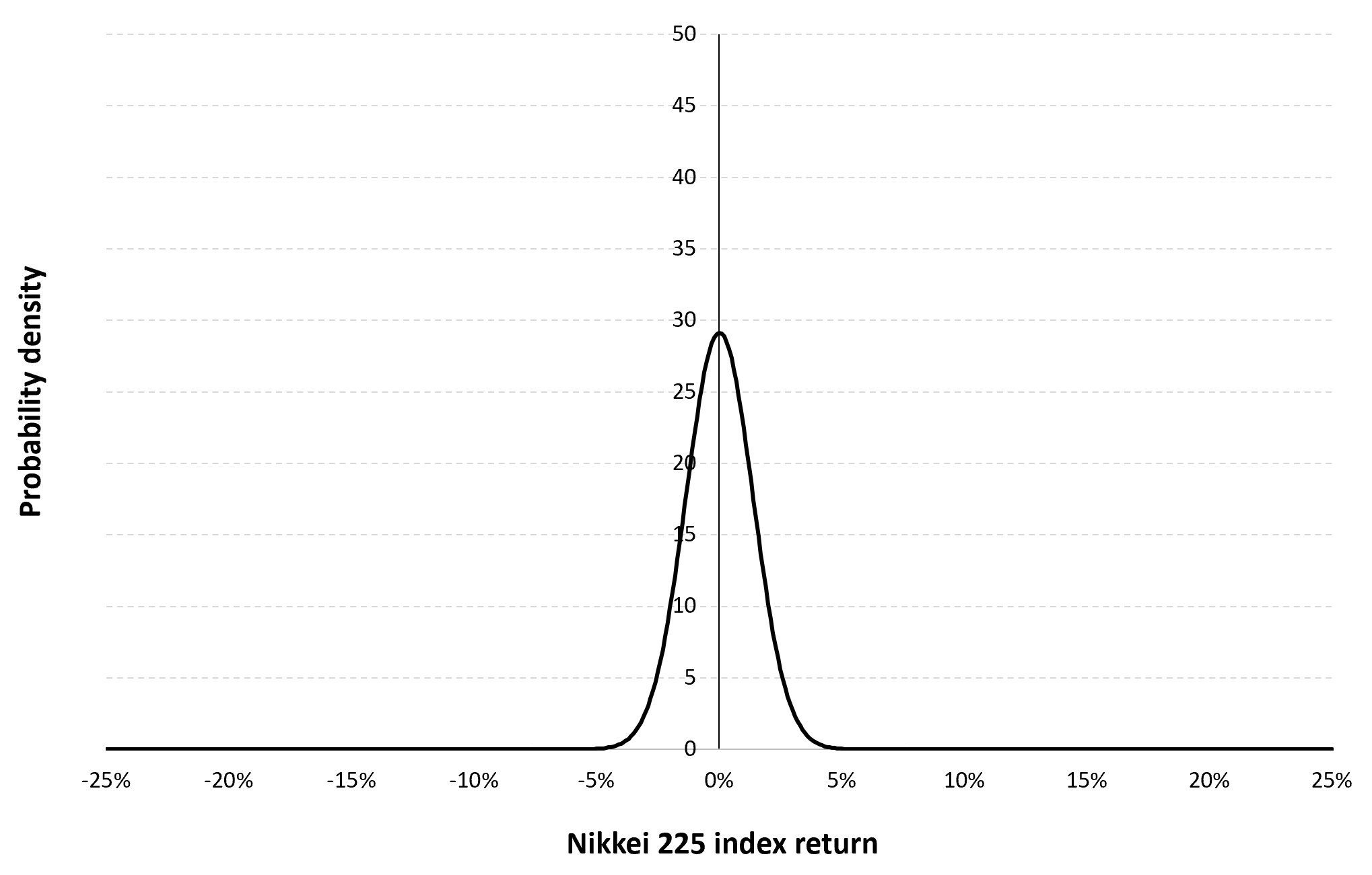
Gaussian distribution
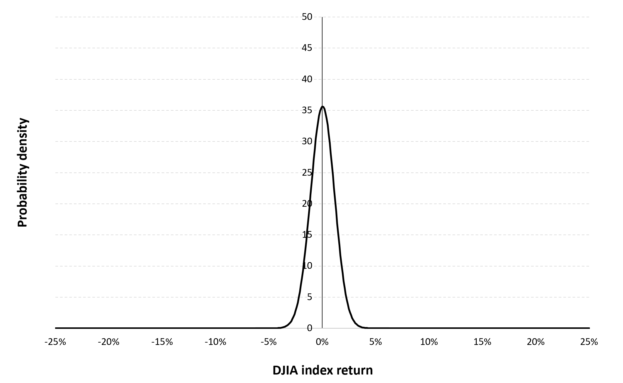
The Gaussian distribution (also called the normal distribution) is a parametric distribution with two parameters: the mean and the standard deviation of returns. We estimated these two parameters over the period from March 1, 1990 to December 30, 2022. The mean of daily returns is equal to 0.02% and the standard deviation of daily returns is equal to 1.37% (or equivalently 3.94% for the annual mean and 28.02% for the annual standard deviation as shown in Table 3 above).
Figure 4 below represents the Gaussian distribution of the Nikkei 225 index daily returns with parameters estimated over the period from March 1, 1990 to December 30, 2022.
Figure 4. Gaussian distribution of the Nikkei 225 index returns.
Source: computation by the author (data: Yahoo! Finance website).
Risk measures of the Nikkei 225 index returns
The R program that you can download above also allows you to compute risk measures about the returns of the Nikkei 225 index.
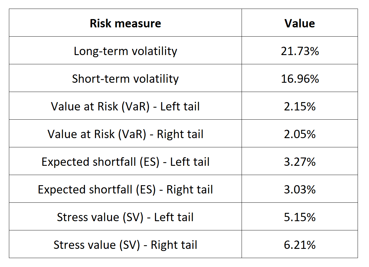
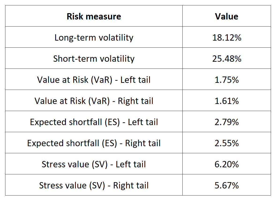
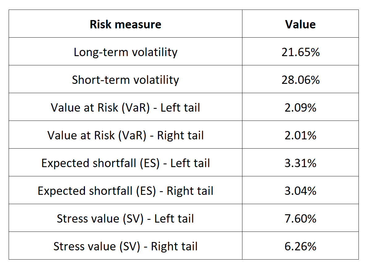
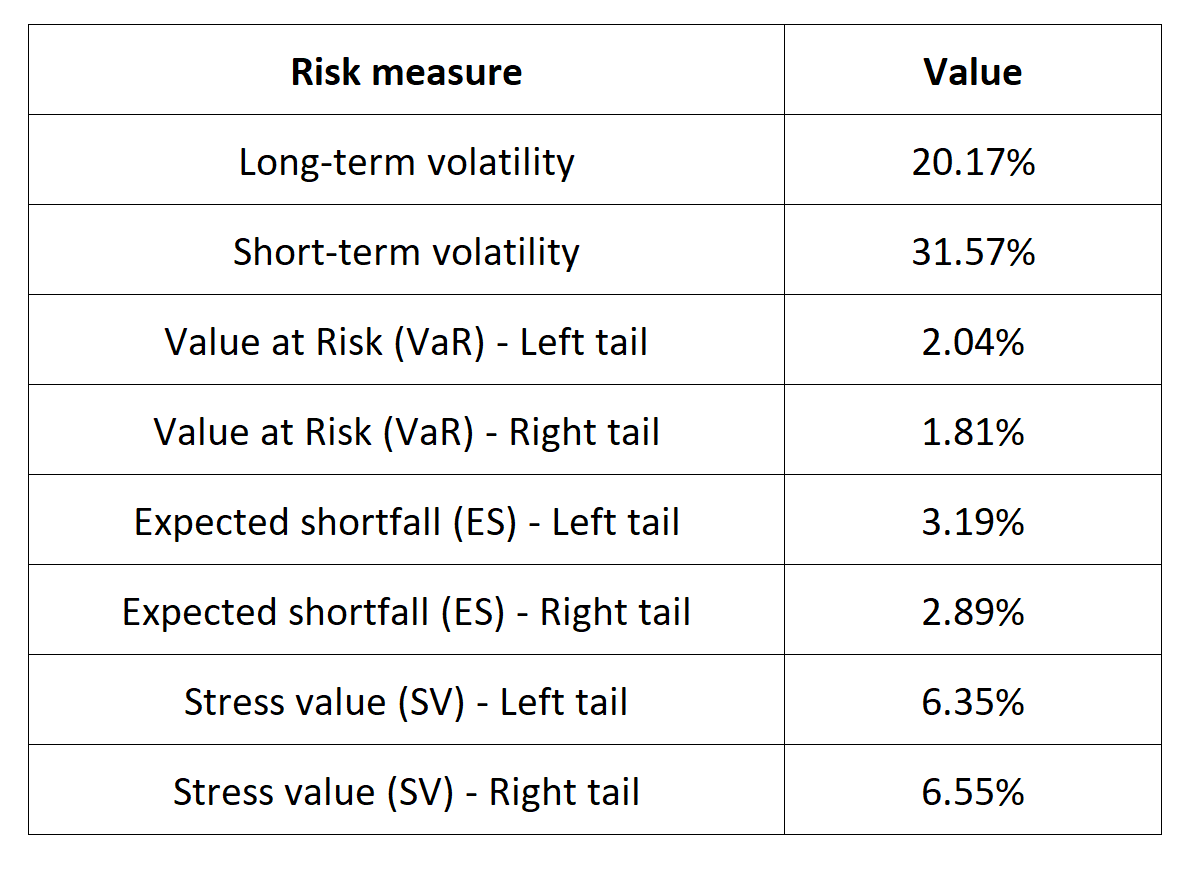
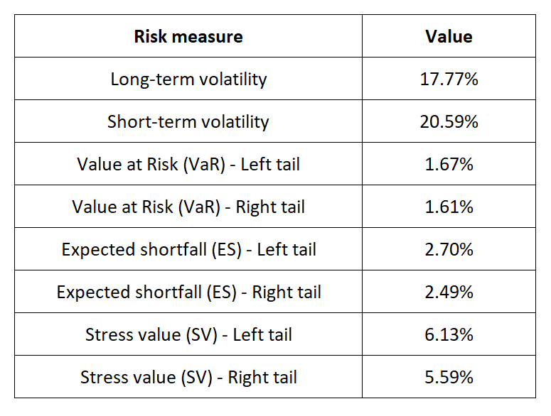
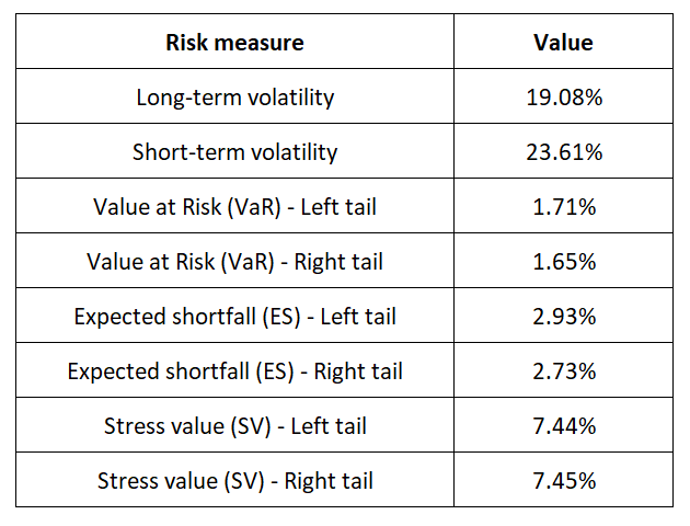
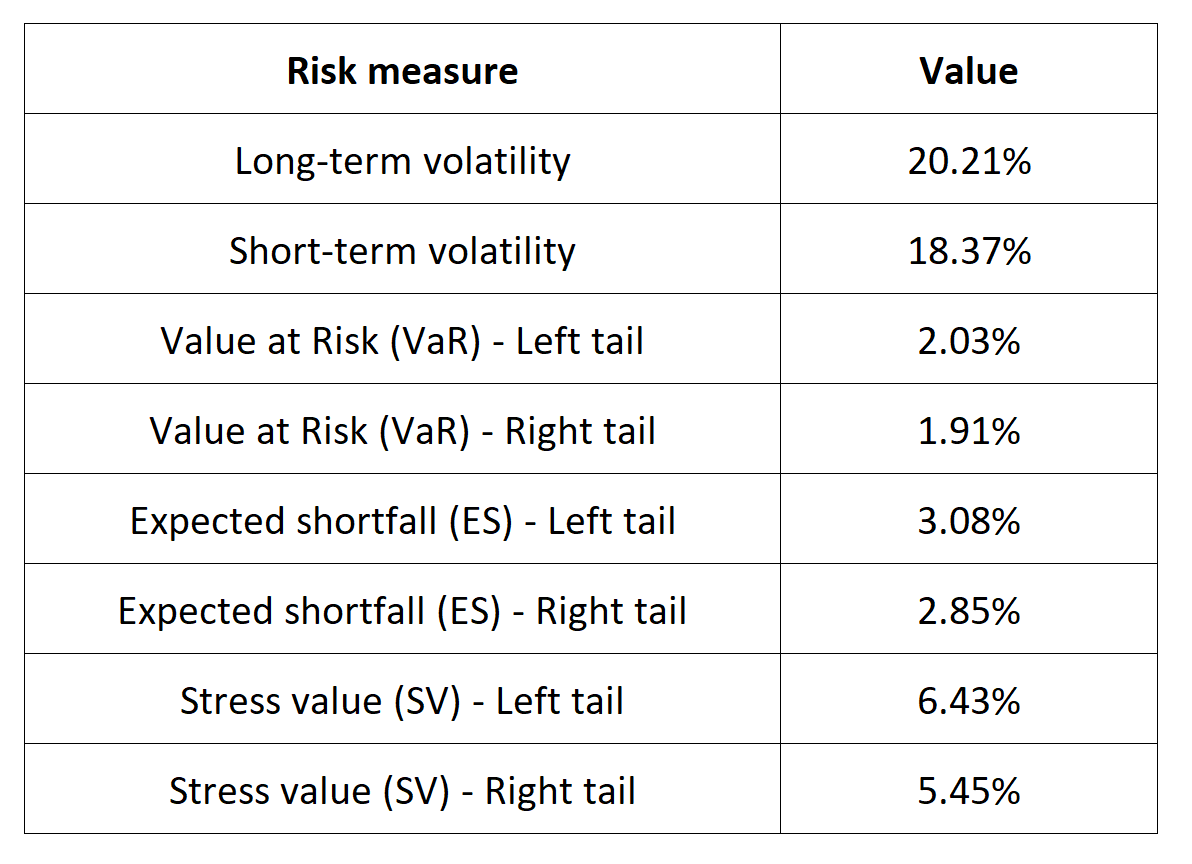
Table 5 below presents the following risk measures estimated for the Nikkei 225 index:
- The long-term volatility (the unconditional standard deviation estimated over the entire period)
- The short-term volatility (the standard deviation estimated over the last three months)
- The Value at Risk (VaR) for the left tail (the 5% quantile of the historical distribution)
- The Value at Risk (VaR) for the right tail (the 95% quantile of the historical distribution)
- The Expected Shortfall (ES) for the left tail (the average loss over the 5% quantile of the historical distribution)
- The Expected Shortfall (ES) for the right tail (the average loss over the 95% quantile of the historical distribution)
- The Stress Value (SV) for the left tail (the 1% quantile of the tail distribution estimated with a Generalized Pareto distribution)
- The Stress Value (SV) for the right tail (the 99% quantile of the tail distribution estimated with a Generalized Pareto distribution)
Table 5. Risk measures for the Nikkei 225 index.
Source: computation by the author (data: Yahoo! Finance website).
The volatility is a global measure of risk as it considers all the returns. The Value at Risk (VaR), Expected Shortfall (ES) and Stress Value (SV) are local measures of risk as they focus on the tails of the distribution. The study of the left tail is relevant for an investor holding a long position in the Nikkei 225 index while the study of the right tail is relevant for an investor holding a short position in the Nikkei 225 index.
Financial maps
You can find financial world maps on the Extreme Events in Finance website. These maps represent the performance, risk and extreme risk in international equity markets.
Figure 5 below represents the world map for extreme risk estimated by the extreme value distribution (see Longin (2016 and 2000)).
Figure 5. Extreme risk map.
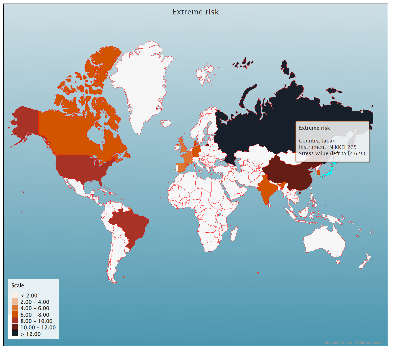
Source: Extreme Events in Finance.
Why should I be interested in this post?
For a number of reasons, management students (as future managers and individual investors) should learn about the Nikkei 225 index. The Nikkei 225 index is a key benchmark for the Japanese equity market, which is one of the world’s largest market. Understanding how the index is constructed, how it performs, and the companies that make up the index is important for anyone studying finance or business in Japan or interested in investing in Japanese equities.
Individual investors can assess the performance of their own investments in the Japanese equity market with the Nikkei 225 index. Last but not least, a lot of asset management firms base their mutual funds and exchange-traded funds (ETFs) on the Nikkei 225 index which can considered as interesting assets to diversify a portfolio. Learning about these products and their portfolio and risk management applications can be valuable for management students.
Related posts on the SimTrade blog
About financial indexes
▶ Nithisha CHALLA Financial indexes
▶ Nithisha CHALLA Calculation of financial indexes
▶ Nithisha CHALLA The business of financial indexes
▶ Nithisha CHALLA Float
Other financial indexes
▶ Nithisha CHALLA The S&P 500 index
▶ Nithisha CHALLA The FTSE 100 index
▶ Nithisha CHALLA The CSI 300 index
▶ Nithisha CHALLA The KOSPI 50 index
About portfolio management
▶ Youssef LOURAOUI Portfolio
▶ Jayati WALIA Returns
About statistics
▶ Shengyu ZHENG Moments de la distribution
▶ Shengyu ZHENG Mesures de risques
Useful resources
Academic research about risk
Longin F. (2000) From VaR to stress testing: the extreme value approach Journal of Banking and Finance, N°24, pp 1097-1130.
Longin F. (2016) Extreme events in finance: a handbook of extreme value theory and its applications Wiley Editions.
Data
Yahoo! Finance Nikkei 225 index
Other
Extreme Events in Finance Risk maps
Wikipedia Nikkei 225
About the author
The article was written in April 2023 by Nithisha CHALLA (ESSEC Business School, Grande Ecole Program – Master in Management, 2021-2023).