

In this article, Youssef LOURAOUI (Bayes Business School,, MSc. Energy, Trade & Finance, 2021-2022) presents the usage of a widely used model for building the yield curve, namely the Nelson-Seigel-Svensson model for interest rate calibration.
This article is structured as follows: we introduce the concept of the yield curve. Next, we present the mathematical foundations of the Nelson-Siegel-Svensson model. Finally, we illustrate the model with practical examples.
Introduction
Fine-tuning the term structure of interest rates is the cornerstone of a well-functioning financial market. For this reason, the testing of various term-structure estimation and forecasting models is an important topic in finance that has received considerable attention for several decades (Lorenčič, 2016).
The yield curve is a graphical representation of the term structure of interest rates (i.e. the relationship between the yield and the corresponding maturity of zero-coupon bonds issued by governments). The term structure of interest rates contains information on the yields of zero-coupon bonds of different maturities at a certain date (Lorenčič, 2016). The construction of the term structure is not a simple task due to the scarcity of zero-coupon bonds in the market, which are the basic elements to estimate the term structure. The majority of bonds traded in the market carry coupons (regular paiement of interests). The yields to maturity of coupon bonds with different maturities or coupons are not immediately comparable. Therefore, a method of measuring the term structure of interest rates is needed: zero-coupon interest rates (i.e. yields on bonds that do not pay coupons) should be estimated from the prices of coupon bonds of different maturities using interpolation methods, such as polynomial splines (e.g. cubic splines) and parsimonious functions (e.g. Nelson-Siegel).
As explained in an interesting paper that I read (Lorenčič, 2016), the prediction of the term structure of interest rates is a basic requirement for managing investment portfolios, valuing financial assets and their derivatives, calculating risk measures, valuing capital goods, managing pension funds, formulating economic policy, making decisions about household finances, and managing fixed income assets . The pricing of fixed income securities such as swaps, bonds and mortgage-backed securities depends on the yield curve. When considered together, the yields of non-defaulting government bonds with different characteristics reveal information about forward rates, which are potentially predictive of real economic activity and are therefore of interest to policy makers, market participants and economists. For instance, forward rates are often used in pricing models and can indicate market expectations of future inflation rates and currency appreciation/depreciation rates. Understanding the relationship between interest rates and the maturity of securities is a prerequisite for developing and testing the financial theory of monetary and financial economics. The accurate adjustment of the term structure of interest rates is the backbone of a well-functioning financial market, which is why the refinement of yield curve modelling and forecasting methods is an important topic in finance that has received considerable attention for several decades (Lorenčič, 2016).
The most commonly used models for estimating the zero-coupon curve are the Nelson-Siegel and cubic spline models. For example, the central banks of Belgium, Finland, France, Germany, Italy, Norway, Spain and Switzerland use the Nelson-Siegel model or a type of its improved extension to fit and forecast yield curves (BIS, 2005). The European Central Bank uses the Sonderlind-Svensson model, an extension of the Nelson-Siegel model, to estimate yield curves in the euro area (Coroneo, Nyholm & Vidova-Koleva, 2011).
Mathematical foundation of the Nelson-Siegel-Svensson model
In this article, we will deal with the Nelson-Siegel extended model, also known as the Nelson-Siegel-Svensson model. These models are relatively efficient in capturing the general shapes of the yield curve, which explains why they are widely used by central banks and market practitioners.
Mathematically, the formula of Nelson-Siegel-Svensson is given by:
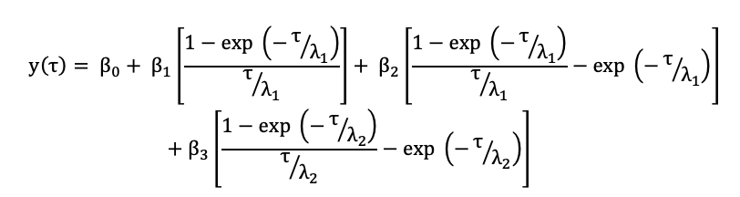
where
- τ = time to maturity of a bond (in years)
- β0 = parameter to capture for the level factor
- β1= parameter to capture the slope factor
- β2 = parameter to capture the curvature factor
- β3 = parameter to capture the magnitude of the second hump
- λ1 and λ2 = parameters to capture the rate of exponential decay
- exp = the mathematical exponential function
The parameters β0, β1, β2, β3, λ1 and λ2 can be calculated with the Excel add-in “Solver” by minimizing the sum of squared residuals between the dirty price (market value, present value) of the bonds and the model price of the bonds. The dirty price is a sum of the clean price, retrieved from Bloomberg, and accrued interest. Financial research propose that the Svensson model should be favored over the Nelson-Siegel model because the yield curve slopes down at the very long end, necessitating the second curvature component of the Svensson model to represent a second hump at longer maturities (Wahlstrøm, Paraschiv, and Schürle, 2022).
Application of the yield curve structure
In financial markets, yield curve structure is of the utmost importance, and it is an essential market indicator for central banks. During my last internship at the Central Bank of Morocco, I worked in the middle office, which is responsible for evaluating risk exposures and profits and losses on the positions taken by the bank on a 27.4 billion euro foreign reserve investment portfolio. Volatility evaluated by the standard deviation, mathematically defined as the deviation of a random variable (asset prices or returns in my example) from its expected value, is one of the primary risk exposure measurements. The standard deviation reveals the degree to which the present return deviates from the expected return. When analyzing the risk of an investment, it is one of the most used indicators employed by investors. Among other important exposures metrics, there is the VaR (Value at Risk) with a 99% confidence level and a 95% confidence level for 1-day and 30-day positions. In other words, the VaR is a metric used to calculate the maximum loss that a portfolio may sustain with a certain degree of confidence and time horizon.
Every day, the Head of the Middle Office arranges a general meeting in which he discusses a global debriefing of the most significant overnight financial news and a debriefing of the middle office desk for “watch out” assets that may present an investment opportunity. Consequently, the team is tasked with adhering to the investment decisions that define the firm, as it neither operates as an investment bank nor as a hedge fund in terms of risk and leverage. As the central bank is tasked with the unique responsibility of safeguarding the national reserve and determining the optimal mix of low-risk assets to invest in, it seeks a good asset strategy (AAA bonds from European countries coupled with American treasury bonds). The investment mechanism is comprised of the segmentation of the entire portfolio into three principal tranches, each with its own features. The first tranche (also known as the security tranche) is determined by calculating the national need for a currency that must be kept safe in order to establish exchange market stability (mostly based on short-term positions in low-risk profile assets) (Liquid and high rated bonds). The second tranche is based on a buy-and-hold strategy and a market approach. The first entails taking a long position on riskier assets than the first tranche until maturity, with no sales during the asset’s lifetime (riskier bonds and gold). The second strategy is based on the purchase and sale of liquid assets with the expectation of better returns.
Participants in the market are accustomed to categorizing the debt of eurozone nations. Germany and the Netherlands, for instance, are regarded as “core” nations, and their debt as safe-haven assets (Figure 1). Due to the stability of their yield spreads, France, Belgium, Austria, Ireland, and Finland are “semi-core” nations (Figure 1). Due to their higher bond yields and more volatile spreads, Spain, Portugal, Italy, and Greece are called “peripheral” (BNP Paribas, 2019) (Figure 2). The 10-year gap represents the difference between a country’s 10-year bond yield and the yield on the German benchmark bond. It is a sign of risk. Therefore, the greater the spread, the greater the risk. Figure 3 represents the yield curve for the Moroccan bond market.
Figure 1. Yield curves for core countries (Germany, Netherlands) and semi-core (France, Austria) of the euro zone.
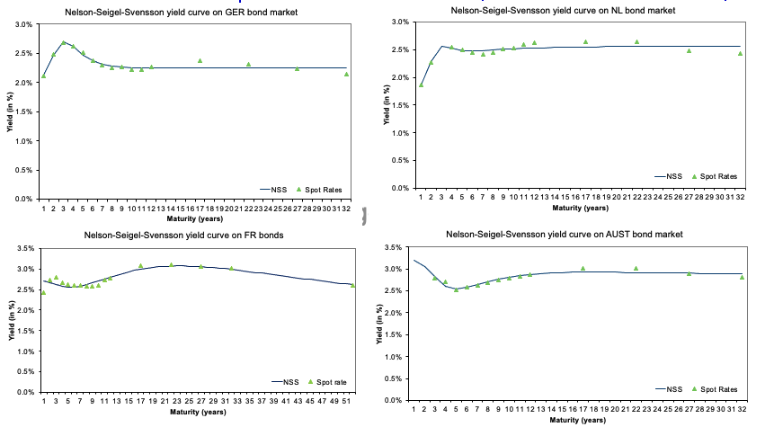
Source: computation by the author.
Figure 2. Yield curves for peripheral countries of the euro zone
(Spain, Italy, Greece and Portugal).
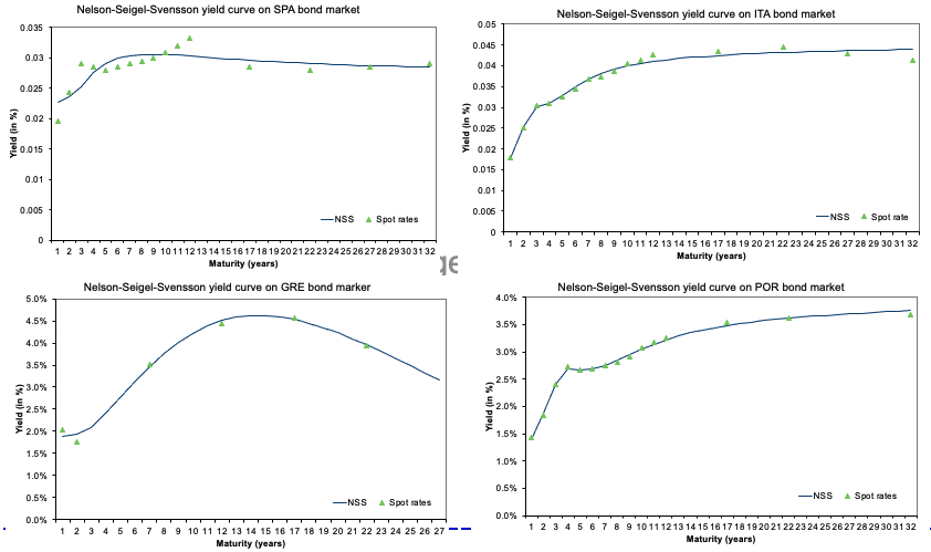
Source: computation by the author.
Figure 3. Yield curve for Morocco.
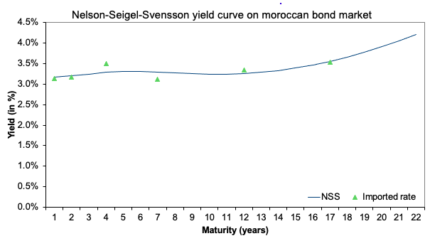
Source: computation by the author.
This example provides a tool comparable to the one utilized by central banks to measure the change in the yield curve. It is an intuitive and simplified model created in an Excel spreadsheet that facilitates comprehension of the investment process. Indeed, it is capable of continuously refreshing the data by importing the most recent quotations (in this case, retrieved from investing.com, a reputable data source).
One observation can be made about the calibration limits of the Nelson-Seigel-Svensson model. In this sense, when the interest rate curve is in negative levels (as in the case of the structure of the Japanese curve), the NSS model does not manage to model negative values, obtaining a result with substantial deviations from spot rates. This can be interpreted as a failure of the NSS calibration approach to model a negative interest rate curve.
In conclusion, the NSS model is considered as one of the most used and preferred models by central banks to obtain the short- and long-term interest rate structure. Nevertheless, this model does not allow to model the structure of the curve for negative interest rates.
Excel file for the calibration model of the yield curve
You can download an Excel file with data to calibrate the yield curve for different countries. This spreadsheet has a special macro to extract the latest data pulled from investing.com website, a reliable source for time-series data.

Why should I be interested in this post?
Predicting the term structure of interest rates is essential for managing investment portfolios, valuing financial assets and their derivatives, calculating risk measures, valuing capital goods, managing pension funds, formulating economic policy, deciding on household finances, and managing fixed income assets. The yield curve affects the pricing of fixed income assets such as swaps, bonds, and mortgage-backed securities. Understanding the yield curve and its utility for the markets can aid in comprehending this parameter’s broader implications for the economy as a whole.
Related posts on the SimTrade blog
Hedge funds
▶ Youssef LOURAOUI Introduction to Hedge Funds
▶ Youssef LOURAOUI Equity market neutral strategy
▶ Youssef LOURAOUI Fixed income arbitrage strategy
▶ Youssef LOURAOUI Global macro strategy
Financial techniques
▶ Bijal GANDHI Interest Rates
▶ Akshit GUPTA Interest Rate Swaps
Other
▶ Youssef LOURAOUI My experience as a portfolio manager in a central bank
Useful resources
Academic research
Lorenčič, E., 2016. Testing the Performance of Cubic Splines and Nelson-Siegel Model for Estimating the Zero-coupon Yield Curve. NGOE, 62(2), 42-50.
Wahlstrøm, Paraschiv, and Schürle, 2022. A Comparative Analysis of Parsimonious Yield Curve Models with Focus on the Nelson-Siegel, Svensson and Bliss Versions. Springer Link, Computational Economics, 59, 967–1004.
Business Analysis
BNP Paribas (2019) Peripheral Debt Offers Selective Opportunities
About the author
The article was written in January 2023 by Youssef LOURAOUI (Bayes Business School,, MSc. Energy, Trade & Finance, 2021-2022).