In this article, Youssef LOURAOUI (Bayes Business School, MSc. Energy, Trade & Finance, 2021-2022) presents the concept of asset allocation, a pillar concept in portfolio management.
This article is structured as follows: we introduce the notion of asset allocation, and we use a practical example to illustrate this notion.
Introduction
An investment portfolio is a collection of assets that are owned by an investor. Individual assets, such as bonds and stocks, as well as asset baskets, such as mutual funds or exchange-traded funds, can be employed. When constructing a portfolio, investors often consider both the projected return and risk. A well-balanced portfolio includes a wide range of investments to benefit from diversification.
The asset allocation is one of the processes in the portfolio construction process. At this point, the investor (or fund manager) must divide the available capital into a number of assets that meet the criteria in terms of risk and return trade-off, while adhering to the investment policy, which specifies the amount of exposure an investor can have and the amount of risk the fund manager can hold in his or her portfolio.
The next phase in the process is to evaluate the risk and return characteristics of the various assets. The analyst develops economic and market expectations that can be used to develop a recommended asset allocation for the customer. The distribution of equities, fixed-income securities, and cash; sub asset classes, such as corporate and government bonds; and regional weightings within asset classes are all decisions that must be taken in the portfolio’s asset allocation. Real estate, commodities, hedge funds, and private equity are examples of alternative assets. Economists and market strategists may set the top-down view on economic conditions and broad market movements. The returns on various asset classes are likely to be altered by economic conditions; for example, equities may do well when economic growth has been surprisingly robust whereas bonds may do poorly if inflation soars. These situations will be forecasted by economists and strategists.
The top-down approach
A top-down approach begins with assessment of macroeconomic factors. The investor examines markets and sectors based on the existing and projected economic climate in order to invest in those that are predicted to perform well. Finally, funding is evaluated for specific companies within these categories.
The bottom up approach
A bottom-up approach focuses on company-specific variables such as management quality and business potential rather than economic cycles or industry analysis. It is less concerned with broad economic trends than top-down analysis is, and instead focuses on company particular.
Types of asset allocations
Arnott and Fabozzi (1992) divide asset allocation into three types: 1) policy asset allocation; 2) dynamic asset allocation; and 3) tactical asset allocation.
Policy asset allocation
The policy asset allocation decision is a long-term asset allocation decision in which the investor aims to assess a suitable long-term “normal” asset mix that represents an optimal mixture of controlled risk and enhanced return. The strategies that offer the best prospects of achieving strong long-term returns are inherently risky. The strategies that offer the greatest safety tend to offer very moderate return opportunities. The balancing of these opposing goals is known as policy asset allocation. The asset mix (i.e., the allocation among asset classes) is mechanistically altered in response to changing market conditions in dynamic asset allocation. Once the policy asset allocation has been established, the investor can focus on the possibility of active deviations from the regular asset mix established by policy. Assume the long-run asset mix is established to be 60% equities and 40% bonds. A variation from this mix under certain situations may be tolerated. A decision to diverge from this mix is generally referred to as tactical asset allocation if it is based on rigorous objective measurements of value. Tactical asset allocation does not consist of a single, well-defined strategy.
Dynamic asset allocation
The term “dynamic asset allocation” can refer to both long-term policy decisions and intermediate-term efforts to strategically position the portfolio to benefit from big market swings, as well as aggressive tactical strategies. As an investor’s risk expectations and tolerance for risk fluctuate, the normal or policy asset allocation may change. It is vital to understand what aspect of the asset allocation decision is being discussed and in what context the words “asset allocation” are being used when delving into asset allocation difficulties.
Tactical asset allocation
Tactical asset allocation broadly refers to active strategies that seek to enhance performance by opportunistically adjusting the asset mix of a port- folio in response to the changing patterns of reward available in the capi- tal markets. Notably, tactical asset allocation tends to refer to disciplined techniques for evaluating anticipated rates of return on various asset classes and constructing an asset allocation response intended to capture larger rewards.
Asset allocation application: an example
For this example, lets suppose the fictitious following scenario with real data involved:
Mr. Dubois recently sold his local home construction company in the south of France to a multinational homebuilder with a nationwide reach. He accepted a job as regional manager for that national homebuilder after selling his company. He is now thinking about the financial future for himself and his family. He is looking forward to his new job, where he enjoys his new role and where he will earn enough money to meet his family’s short- and medium-term liquidity demands. He feels strongly that he should not invest the profits of the sale of his company in real estate because his income currently rely on the state of the real estate market. He speaks with a financial adviser at his bank about how to invest his money so that he can retire comfortably in 20 years.
The initial portfolio objective they created seek a nominal return goal of 7% with a Sharpe ratio of at least 1 (for this example, we consider the risk-free rate to be equal to zero). The bank’s asset management division gives Mr Dubois and his adviser with the following data (Figure 1) on market expectations.
Figure 1. Risk, return and correlation estimates on market expectation.
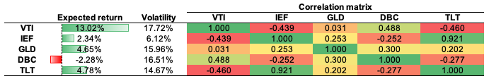
Source: computation by the author (Data: Refinitiv Eikon).
In order to replicate a global asset allocation approach, we shortlisted a number of trackers that would represent our investment universe. To keep a well-balanced approach, we took trackers that would represent the main asset classes: global equities (VTI – Vanguard Total Stock Market ETF), bonds (IEF – iShares 7-10 Year Treasury Bond ETF and TLT – iShares 20+ Year Treasury Bond ETF) and commodities (DBC – Invesco DB Commodity Index Tracking Fund and GLD – SPDR Gold Shares). To create the optimal asset allocation, we extracted the equivalent of a ten-year timeframe from Refinitiv Eikon to capture the overall performance of the portfolio in the long run. As captured in Figure 1, the global equities was the best performing asset class during the period covered (13.02% annualised return), followed by long term bond (4.78% annualised return) and by gold (4.65% annualised return).
Figure 2. Asset class performance (rebased to 100).
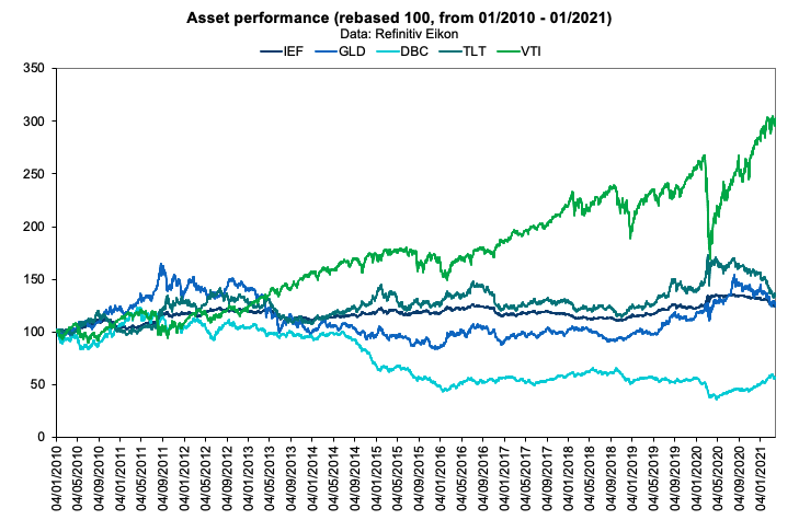
Source: computation by the author (Data: Refinitiv Eikon).
After analyzing the historical return on the assets retained, as well as their volatility and covariance (and correlation), we can apply Mean-Variance portfolio optimization to determine the optimal portfolio. The optimal asset allocation would be the end outcome of the optimization procedure. The optimal portfolio, according to Markowitz’ seminal study on portfolio construction, will seek to create the best risk-return trade-off for an investor. After performing the calculations, we notice that investing 42.15% in the VTI fund, 30.69% in the IEF fund, 24.88% in the TLT fund, and 2.28% in the GLD fund yields the best asset allocation. As reflected in this asset allocation, the investor intends to invest his assets in a mix of equities (about 43%) and bonds (approximately 55%), with a marginal position (around 3%) in gold, which is widely employed in portfolio management as an asset diversifier due to its correlation with other asset classes. As captured by this asset allocation, we can clearly see the defensive nature of this portfolio, which relies significantly on the bond part of the allocation to operate as a hedge while relying on the equities part as the main driver of returns.
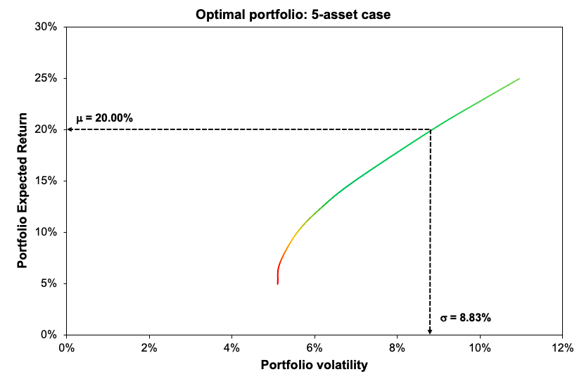
As shown in Figure 3, the optimal asset allocation has a better Sharpe ratio (1.27 vs 0.62) and is captured farther along the efficient frontier line than a naive equally-weighted allocation . The only portfolio with the needed characteristics is the optimal one, as the investor’s goal was to attain a 7% projected return with a minimum Sharpe ratio of 1.
Figure 3. Optimal asset allocation and the Efficient Frontier plot.
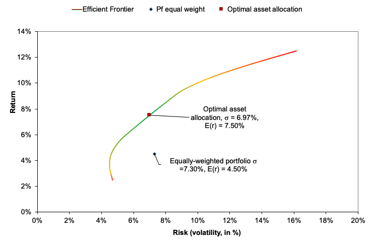
Source: computation by the author (Data: Refinitiv Eikon).
Will this allocation, however, continue to perform well in the future? The market’s reliance on future expectations, return, volatility, and correlation predictions, as well as the market regime, will ultimately determine how much the performance predicted by this study will really change in the future.
Excel file for asset allocation
You can find below the Excel spreadsheet that complements the example above.

Why should I be interested in this post?
The purpose of portfolio management is to maximize (expected) returns on the entire portfolio, not just on one or two stocks for a given level of risk. By monitoring and maintaining your investment portfolio, you can build a substantial amount of wealth for a variety of financial goals, such as retirement planning. This post facilitates comprehension of the fundamentals underlying portfolio construction and investing.
Related posts on the SimTrade blog
▶ Youssef LOURAOUI Markowitz Modern Portfolio Theory
▶ Youssef LOURAOUI Optimal portfolio
▶ Youssef LOURAOUI Portfolio
Useful resources
Academic research
Arnott, R. D., and F. J. Fabozzi. 1992. The many dimensions of the asset allocation decision. In Active asset allocation, edited by R. Arnott and F. J. Fabozzi. Chicago: Probus Publishing.
Fabozzi, F.J., 2009. Institutional Investment Management: Equity and Bond Portfolio Strategies and Applications. I (4-6). John Wiley and Sons Edition.
Pamela, D. and Fabozzi, F., 2010. The Basics of Finance: An Introduction to Financial Markets, Business Finance, and Portfolio Management. John Wiley and Sons Edition.
About the author
The article was written in December 2022 by Youssef LOURAOUI (Bayes Business School, MSc. Energy, Trade & Finance, 2021-2022).


 Source: computation by the author.
 Source: computation by the author.
 Source: computation by the author.
 Source: computation by the author.
 Source: computation by the author.
 Source: computation by the author.
 Source: computation by the author.
 Source: computation by the author.
 Source: computation by the author.


 Source : computation by the author.