

This article written by Akshit GUPTA (ESSEC Business School, Grande Ecole Program – Master in Management, 2019-2022) presents the strategies of straddle and strangle based on options.
Introduction
In financial markets, hedging is implemented by investors to minimize the risk exposure and maximize the returns for any investment in securities. While hedging does not necessarily eliminate the entire risk for an investment, it does limit or offset any potential losses that the investor can incur.
Option contracts are commonly used by investors / traders as hedging mechanisms due to their great flexibility (in terms of expiration date, moneyness, liquidity, etc.) and availability. Positions in options are used to offset the risk exposure in the underlying security, another option contract or in any other derivative contract. Option strategies can be directional or non-directional.
Directional strategy is when the investor has a specific viewpoint about the movement of an asset price and aims to earn profit if the viewpoint holds true. For instance, if an investor has a bullish viewpoint about an asset and speculates that its price will rise, she/he can buy a call option on the asset, and this can be referred as a directional trade with a bullish bias. Similarly, if an investor has a bearish viewpoint about an asset and speculates that its price will fall, she/he can buy a put option on the asset, and this can be referred as a directional trade with a bearish bias.
On the other hand, non-directional strategies can be used by investors when they anticipate a major market movement and want to gain profit irrespective of whether the asset price rises or falls, i.e., their payoff is independent of the direction of the price movement of the asset but instead depends on the magnitude of the price movement. There are various popular non-directional strategies that can be implemented through a combination of option contracts to minimize risk and maximize returns. In this post, we are interested in straddle and strangle.
Straddle
In a straddle, the investor buys a European call and a European put option, both at the same expiration date and at the same strike price. This strategy works in a similar manner like a strangle (see below). However, the potential losses are a bit higher than incurred in a strangle if the stock price remains near the central value at expiration date.
A long straddle is when the investor buys the call and put options, whereas a short straddle is when the investor sells the call and put options. Thus, whether a straddle is long or short depends on whether the options are long or short.
Market Scenario
When the price of underlying is expected to move up or down sharply, investors chose to go for a long straddle and the expiration date is chosen such that it occurs after the expected price movement. Scenarios when a long straddle might be used can include budget or company earnings declaration, war announcements, election results, policy changes etc.
Conversely, a short straddle can be implemented when investors do not expect a significant movement in the asset prices.
Example
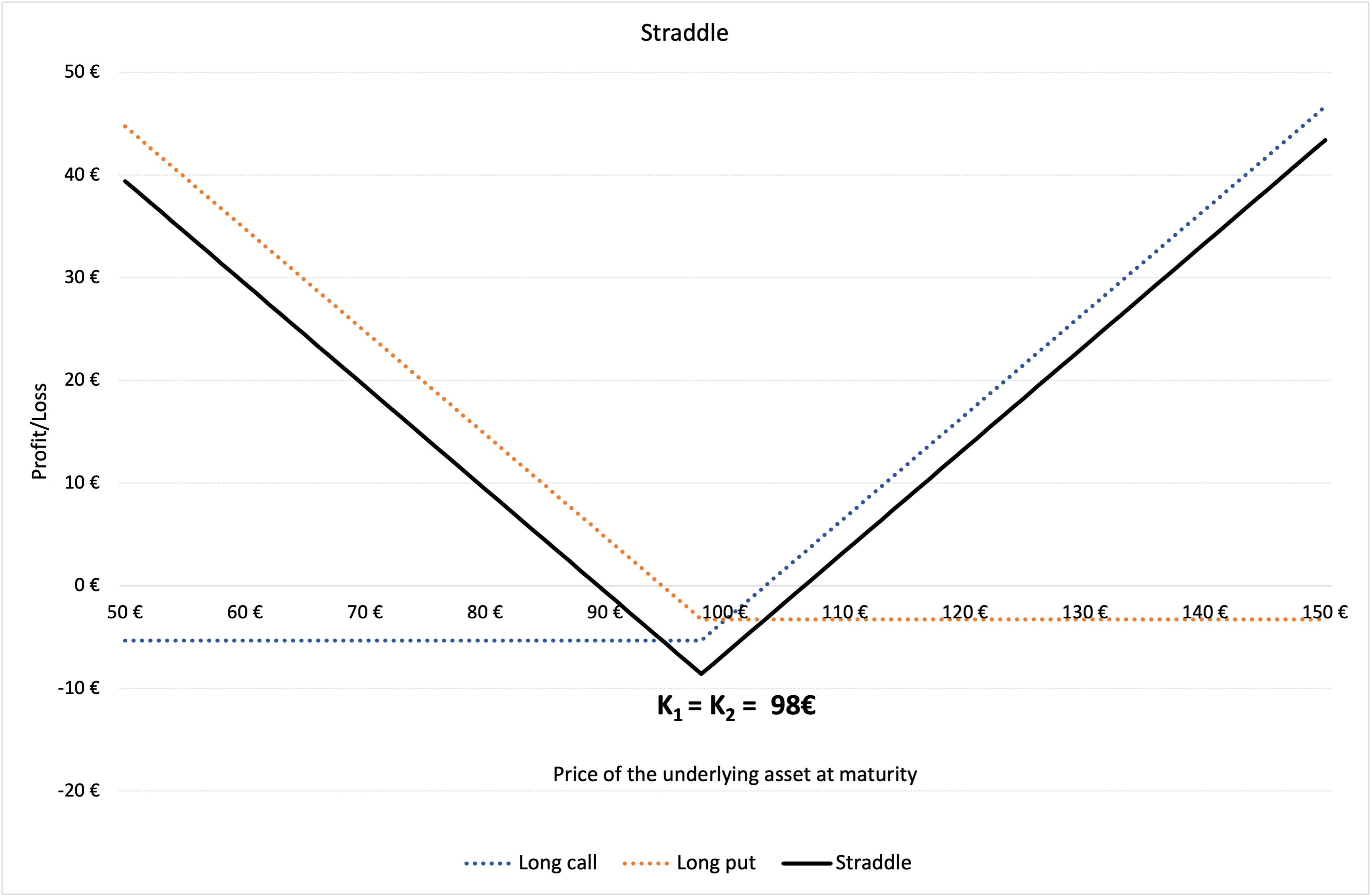
In Figure 1 below, we represent the profit and loss function of a straddle strategy using a long call and a long put option. K1 is the strike price of the long call i.e., €98 and K2 is the strike price of the long put position i.e., €98. The premium of the long call is equal to €5.33, and the premium of the long put is equal to €3.26 computed using the Black-Scholes-Merton model. The time to maturity (T) is of 18 days (i.e., 0.071 years). At the time of valuation, the price of the underlying asset (S0) is €100, the volatility (σ) of the underlying asset is 40% and the risk-free rate (r) is 1% (market data).
Figure 1. Profit and loss (P&L) function of a straddle position.
Source: computation by the author.
You can download below the Excel file for the computation of the straddle value using the Black-Scholes-Merton model.

Strangle
In a strangle, the investor buys a European call and a European put option, both at the same expiration date but different strike prices. To benefit from this strategy, the price of the underlying asset must move further away from the central value in either direction i.e., increase or decrease. If the stock prices stay at a level closer to the central value, the investor will incur losses.
Like a straddle, a long strangle is when the investor buys the call and put options, whereas a short strangle is when the investor sells (issues) the call and put options. The only difference is the strike price, as in a strangle, the call option has a higher strike price than the price of the underlying asset, while the put option has a lower strike price than the price of the underlying asset.
Strangles are generally cheaper than straddles because investors require relatively less price movement in the asset to ‘break even’.
Market Scenario
The long strangle strategy can be used when the trader expects that the underlying asset is likely to experience significant volatility in the near term. It is a limited risk and unlimited profit strategy because the maximum loss is limited to the net option premiums while the profits depend on the underlying price movements.
Similarly, short strangle can be implemented when the investor holds a neutral market view and expects very little volatility in the underlying asset price in the near term. It is a limited profit and unlimited risk strategy since the payoff is limited to the premiums received for the options, while the risk can amount to a great loss if the underlying price moves significantly.
Example
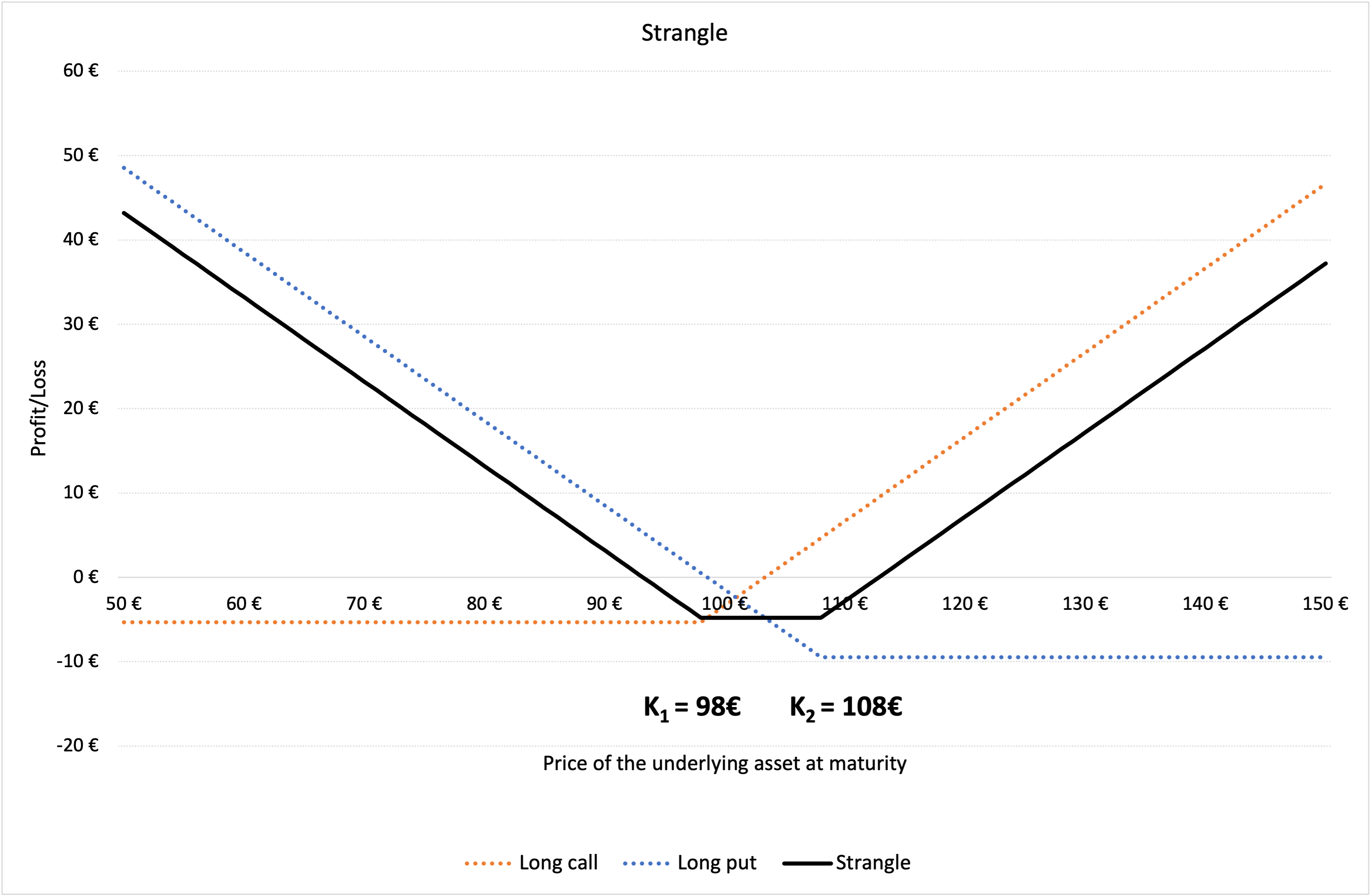
In Figure 2 below, we represent the profit and loss function of a strangle strategy using a long call and a long put option. K1 is the strike price of the long call i.e., €98 and K2 is the strike price of the long put position i.e., €108. The premium of the long call is equal to €5.33, and the premium of the long put is equal to €9.47 computed using the Black-Scholes-Merton model. The time to maturity (T) is of 18 days (i.e., 0.071 years). At the time of valuation, the price of the underlying asset (S0) is €100, the volatility (σ) of the underlying asset is 40% and the risk-free rate (r) is 1% (market data).
Figure 2. Profit and loss (P&L) function of a strangle position.
Source: computation by the author..
You can download below the Excel file for the computation of the strangle value using the Black-Scholes-Merton model.
Related Posts
▶ Akshit GUPTA Options
▶ Akshit GUPTA The Black-Scholes-Merton model
▶ Akshit GUPTA Option Spreads
▶ Akshit GUPTA Option Trader – Job description
Useful resources
Academic research articles
Black F. and M. Scholes (1973) “The Pricing of Options and Corporate Liabilities” The Journal of Political Economy, 81, 637-654.
Merton R.C. (1973) “Theory of Rational Option Pricing” Bell Journal of Economics, 4, 141–183.
Books
Hull J.C. (2015) Options, Futures, and Other Derivatives, Ninth Edition, Chapter 10 – Trading strategies involving Options, 276-295.
Wilmott P. (2007) Paul Wilmott Introduces Quantitative Finance, Second Edition, Chapter 8 – The Black Scholes Formula and The Greeks, 182-184.
About the author
Article written in January 2022 by Akshit GUPTA (ESSEC Business School, Grande Ecole Program – Master in Management, 2019-2022).