

This article written by Akshit GUPTA (ESSEC Business School, Grande Ecole Program – Master in Management, 2019-2022) presents the concept of protective put using option contracts.
Introduction
Hedging is a strategy implemented by investors to reduce the risk in an existing investment. In financial markets, hedging is an effective tool used by investors to minimize the risk exposure and change the risk profile for any investment in securities. While hedging does not necessarily eliminate the entire risk for any investment, it does limit the potential losses that the investor can incur.
Option contracts are commonly used by market participants (traders, investors, asset managers, etc.) as hedging mechanisms due to their great flexibility (in terms of expiration date, moneyness, liquidity, etc.) and availability. Positions in options are used to offset the risk exposure in the underlying security, another option contract or in any other derivative contract. There are various popular strategies that can be implemented through option contracts to minimize risk and maximize returns, one of which is a protective put.
Buying a protective put
A put option gives the buyer of the option, the right but not the obligation, to sell a security at a predefined date and price.
A protective put also called as a synthetic long option, is a hedging strategy that limits the downside of an investment. In a protective put, the investor buys a put option on the stock he/she holds in its portfolio. The protective put option acts as a price floor since the investor can sell the security at the strike price of the put option if the price of the underlying asset moves below the strike price. Thus, the investor caps its losses in case the underlying asset price moves downwards. The investor has to pay an option premium to buy the put option.
The maximum payoff potential from using this strategy is unlimited and the potential downside/losses is limited to the strike price of the put option.
Market scenario
A put option is generally bought to safeguard the investment when the investor is bullish about the market in the long run but fears a temporary fall in the prices of the asset in the short term.
For example, an investor owns the shares of Apple and is bullish about the stock in the long run. However, the earnings report for Apple is due to be released by the end of the month. The earnings report can have a positive or a negative impact on the prices of the Apple stock. In this situation, the protective put saves the investor from a steep decline in the prices of the Apple stock if the report is unfavorable.
Let us consider a protective position with buying at-the money puts. One of following three scenarios may happen:
Scenario 1: the stock price does not change, and the puts expire at the money.
In this scenario, the market viewpoint of the investor does not hold correct and the loss from the strategy is the premium paid on buying the put options. In this case, the option holder does not exercise its put options, and the investor gets to keep the underlying stocks.
Scenario 2: the stock price rises, and the puts expire in the money.
In this scenario, since the price of the stock was locked in through the put option, the investor enjoys a short-term unrealized profit on the underlying position. However, the put option will not be exercised by the investor and it will expire worthless. The investor will lose the premium paid on buying the puts.
Scenario 3: the stock price falls, and the puts expire out of the money.
In this scenario, since the price of the stock was locked in through the put option, the investor will execute the option and sell the stocks at the strike price. There is protection from the losses since the investor holds the put option.
Risk profile
In a protective put, the total cost of the investment is equal to the price of the underlying asset plus the put price. However, the profit potential for the investment is unlimited and the maximum losses are capped to the put option price. The risk profile of the position is represented in Figure 1.
Figure 1. Profit or Loss (P&L) function of the underlying position and protective put position.
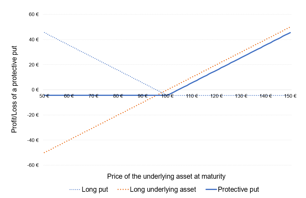
Source: computation by the author.
You can download below the Excel file for the computation of the Profit or Loss (P&L) function of the underlying position and protective put position.

The delta of the position is equal to the sum of the delta of the long position in the underlying asset (+1) and the long position in the put option (Δ). The delta of a long put option is negative which implies that a fall in the asset price will result in an increase in the put price and vice versa. However, the delta of a protective put strategy is positive. This implies that in a protective put strategy, the value of the position tends to rise when the underlying asset price increases and falls when the underlying asset prices decreases.
Figure 2 represents the delta of the protective put position as a function of the price of the underlying asset. The delta of the put option is computed with the Black-Scholes-Merton model (BSM model).
Figure 2. Delta of a protective put position.
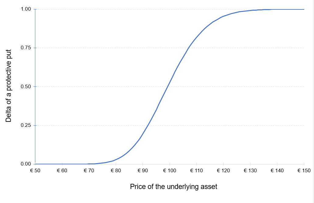
Source: computation by the author (based on the BSM model).
You can download below the Excel file for the computation of the delta of a protective put position.
Example
An investor holds 100 shares of Apple bought at the current price of $144 each. The total initial investment is equal to $14,400. He is skeptical about the effect of the upcoming earnings report of Apple by the end of the current month. In order to avoid losses from a possible downside in the price of the Apple stock, he decides to purchase at-the-money put options on the Apple stock (lot size is 100) with a maturity of one month, using the protective put strategy.
We use the following market data: the current price of Appel stock is $144, the implied volatility of Apple stock is 22.79% and the risk-free interest rate is equal to 1.59%.
Based on the Black-Scholes-Merton model, the price of the put option $3.68.
Let us consider three scenarios at the time of maturity of the put option:
Scenario 1: stability of the price of the underlying asset at $144
The market value of the investment $14,400. The total cost of the initial investment is the cost of acquiring the Apple stocks ($14,400) plus the cost of buying the put options ($368 = $3.68*100), which is equal to $14,768, (i.e. ($14,400 + $368)).
As the stock price is stable at $144, the investor will not execute the put option and the option will expire worthless.
By not executing the put option, the investor incurs a loss which is equal to the price of the put option which is $368.
Scenario 2: an increase in the price of the underlying asset to $155
The market value of the investment $15,500. The total cost of the initial investment is the cost of acquiring the Apple stocks ($14,400) plus the cost of buying the put options ($368 = $3.68*100), which is equal to $14,768, (i.e. ($14,400 + $368)).
As the stock price is at $155, the investor will not execute the put option and hold on the underlying stock.
By not executing the put option, the investor incurs a loss which is equal to the price of the put option which is $368.
Scenario 3: a decrease in the price of the underlying asset to $140
The market value of the investment $14,000. The total cost of the initial investment is the cost of acquiring the Apple stocks ($14,400) plus the cost of buying the put options ($368 = $3.68*100), which is equal to $14,768, (i.e. ($14,400 + $368)).
As the stock price has decreased to $140, the investor will execute the put option and sell the Apple stocks at $144. By executing the put option, the investor will protect himself from incurring a loss of $400 (i.e.($144-$140)*100) due to a decrease in the Apple stock prices.
Related Posts
▶ Akshit GUPTA Options
▶ Akshit GUPTA The Black-Scholes-Merton model
▶ Akshit GUPTA Option Greeks – Delta
▶ Akshit GUPTA Covered call
▶ Akshit GUPTA Option Trader – Job description
Useful Resources
Black F. and M. Scholes (1973) “The Pricing of Options and Corporate Liabilities” The Journal of Political Economy, 81, 637-654.
Hull J.C. (2015) Options, Futures, and Other Derivatives, Ninth Edition, Chapter 10 – Trading strategies involving Options, 276-295.
Merton R.C. (1973) “Theory of Rational Option Pricing” Bell Journal of Economics, 4(1): 141–183.
Wilmott P. (2007) Paul Wilmott Introduces Quantitative Finance, Second Edition, Chapter 8 – The Black Scholes Formula and The Greeks, 182-184.
About the author
Article written in January 2022 by Akshit GUPTA (ESSEC Business School, Grande Ecole Program -Master in Management, 2019-2022).