

This article written by Akshit GUPTA (ESSEC Business School, Grande Ecole Program – Master in Management, 2019-2022) presents the different option spreads used to hedge a position in financial markets.
Introduction
In financial markets, hedging is implemented by investors to minimize the risk exposure for any investment in securities. While hedging does not necessarily eliminate the entire risk for an investment, it does limit or offset any potential losses that the investor can incur.
Option contracts are commonly used by traders and investors as hedging mechanisms due to their great flexibility (in terms of expiration date, moneyness, liquidity, etc.) and availability. Positions in options are used to offset the risk exposure in the underlying security, another option contract or in any other derivative contract. Option strategies can be directional or non-directional.
Spreads are hedging strategies used in trading in which traders buy and sell multiple option contracts on the same underlying asset. In a spread strategy, the option type used to create a spread has to be consistent, either call options or put options. These are used frequently by traders to minimize their risk exposure on the positions in the underlying assets.
Bull Spread
In a bull spread, the investor buys a European call option on the underlying asset with strike price K1 and sells a call option on the same underlying asset with strike price K2 (with K2 higher than K1) with the same expiration date. The investor expects the price of the underlying asset to go up and is bullish about the stock. Bull spread is a directional strategy where the investor is moderately bullish about the underlying asset, she is investing in.
When an investor buys a call option, there is a limited downside risk (the loss of the premium) and an unlimited upside risk (gains). The bull spread reduces the potential downside risk on buying the call option, but also limits the potential profit by capping the upside. It is used as an effective hedge to limit the losses.
Market Scenario
When the price of underlying asset is expected to moderately move up, investors chose to execute a bull spread and the expiration date is chosen such that it occurs after the expected price movement. If the price decreases significantly by the expiration of the call options, the investor loses money by using a bull spread.
Example
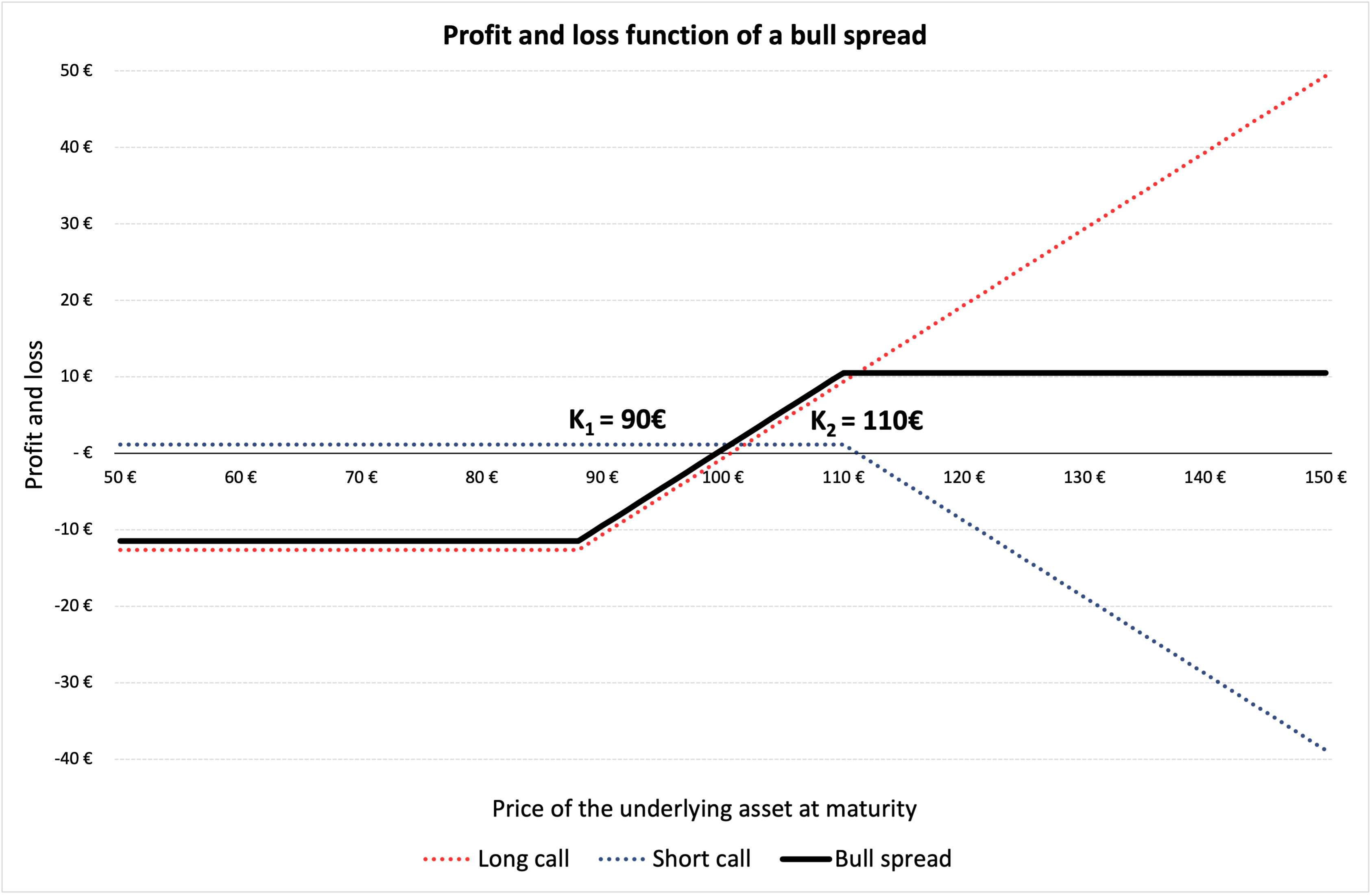
In Figure 1 below, we represent the profit and loss function of a bull spread strategy using a long and a short call option. K1 is the strike price of the long call i.e., €88 and K2 is the strike price of the short call position i.e., €110. The premium of the long call is equal to €12.62, and the premium of the short call is equal to €1.16 computed using the Black-Scholes-Merton model. The time to maturity (T) is of 18 days (i.e., 0.071 years). At the time of valuation, the price of the underlying asset (S0) is €100, the volatility (σ) of the underlying asset is 40% and the risk-free rate (r) is 1% (market data).
Figure 1. Profit and loss (P&L) function of a bull spread.
Source: computation by the author.
You can download below the Excel file for the computation of the bull spread value using the Black-Scholes-Merton model.

Bear Spread
In a bear spread, the investor expects the price of the underlying asset to moderately decline in the near future. In order to hedge against the downside, the investor buys a put option with strike price K1 and sells another put option with strike price K2, with K1 lower than < K2. Initially, this initial position leads to a cash outflow since the put option bought (with strike price K1) has a higher premium than put option sold (with strike price K2) as K1 is lower than < K2.
Market Scenario
When the price of underlying asset is expected to moderately move down, investors chose to execute a bear spread and the expiration date is chosen such that it occurs after the expected price movement. Bear spread is a directional strategy where the investor is moderately bearish about the stock he is investing in. If the price increases significantly by the expiration of the put options, the investor loses money by using a bear spread.
Example
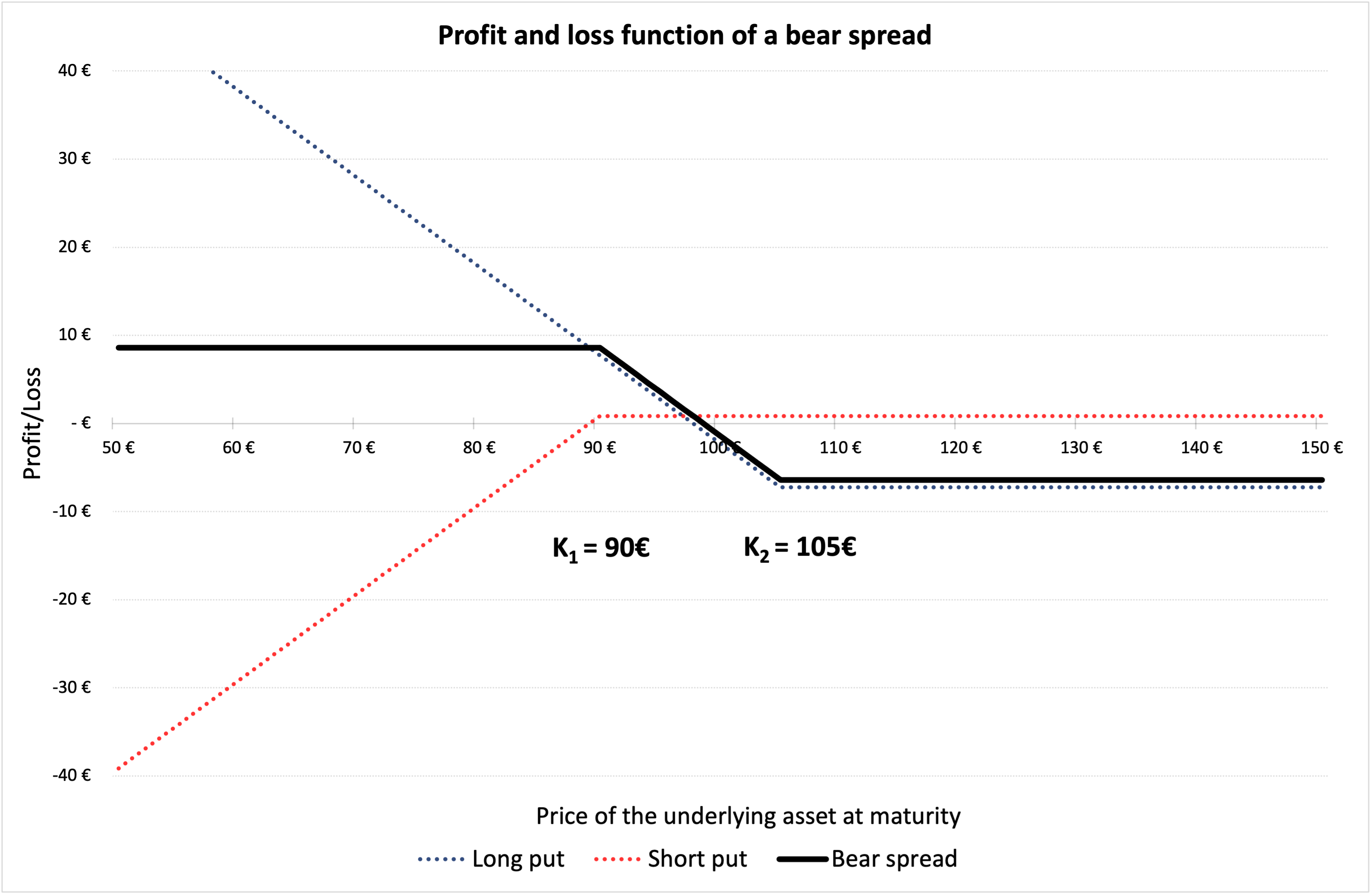
In Figure 2 below, we represent the profit and loss function of a bear spread strategy using a long and a short put option. K1 is equal to the strike price of the short put i.e., €90 and K2 is equal to the strike price of the long put i.e., €105. The premium of the short put is equal to €0.86, and the premium long put is equal to €7.26 computed using the Black-Scholes-Merton model.
The time to maturity (T) is of 18 days (i.e., 0.071 years). At the time of valuation, the price of the underlying asset (S0) is €100, the volatility (σ) of stock is 40% and the risk-free rate (r) is 1% (market data).
Figure 2. Profit and loss (P&L) function of a bear spread.
Source: computation by the author.
You can download below the Excel file for the computation of the bear spread value using the Black-Scholes-Merton model.
Butterfly Spread
In a butterfly spread, the investor expects the price of the underlying asset to remain close to its current market price in the near future. Just as a bull and bear spread, a butterfly spread can be created using call options. In order to profit from the expected market scenario, the investor buys a call option with strike price K1 and buys another call option with strike price K3, where K1 < K3, and sells two call options at price K2, where K1 < K2 < K3. Initially, this initial position leads to a net cash outflow.
Market Scenario
When the price of underlying asset is expected to stay stable, investors chose to execute a butterfly spread and the expiration date is chosen such that the expected price movement occurs before the expiration date. Butterfly spread is a non-directional strategy where the investor expects the price to remain stable and close to the current market price. If the price movement is significant (either downward or upward) by the expiration of the call options, the investor loses money by using a butterfly spread.
Example
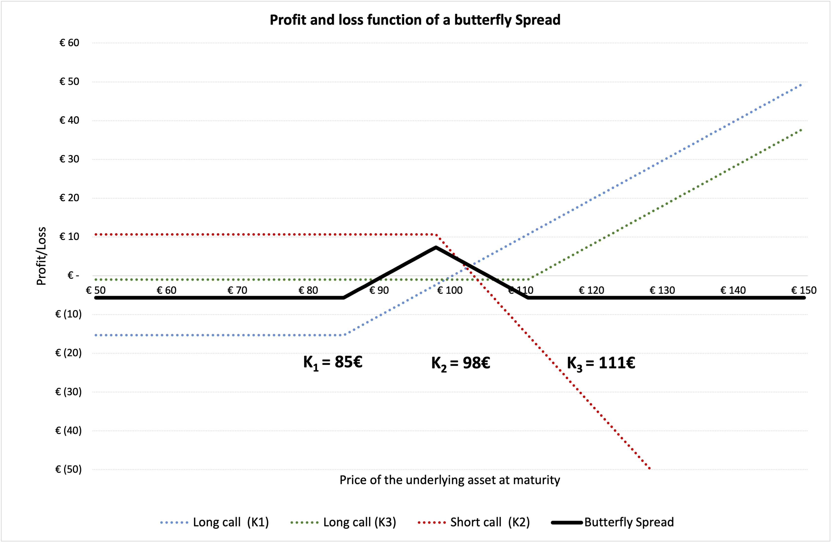
In Figure 3 below, we represent the profit and loss function of a butterfly spread strategy using call options. K1 is equal to the strike price of the long call position i.e., €85 and K2 is equal the strike price of the two short call positions i.e., €98 and K3 is equal to the strike price of another long call position i.e., €111. The premium of the long call K1 is equal to €15.332, the premium of the long call K3 is equal to €0.993 and the premium of the short call K2 is equal to €5.334 computed using the Black-Scholes-Merton model. The premium of the butterfly spread is then equal to €5.657 (= 15.332 + 0.993 -2*5.334), which corresponds to an outflow for the investor.
The time to maturity (T) is of 18 days (i.e., 0.071 years). At the time of valuation, the price of the (S0) is €100, the volatility (σ) of stock is 40% and the risk-free rate (r) is 1% (market data).
Figure 3. Profit and loss (P&L) function of a butterfly spread.
Source: computation by the author.
You can download below the Excel file for the computation of the butterfly spread value using the Black-Scholes-Merton model.
Note that bull, bear, and butterfly spreads can also be created from put options or a combination of call and put options.
Related posts
▶ Gupta A. Options
▶ Gupta A. The Black-Scholes-Merton model
▶ Gupta A. Option Greeks – Delta
▶ Gupta A. Hedging Strategies – Equities
Useful resources
Hull J.C. (2018) Options, Futures, and Other Derivatives, Tenth Edition, Chapter 12 – Trading strategies involving Options, 282-301.
About the author
Article written in January 2022 by Akshit GUPTA (ESSEC Business School, Grande Ecole Program – Master in Management, 2019-2022).