Extreme returns and tail modelling of the S&P 500 index for the US equity market

In this article, Shengyu ZHENG (ESSEC Business School, Grande Ecole Program – Master in Management, 2020-2024) describes the statistical behavior of extreme returns of the S&P 500 index for the US equity market and explains how extreme value theory can be used to model the tails of its distribution.
The S&P 500 index for the US equity market
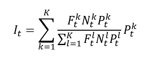
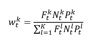
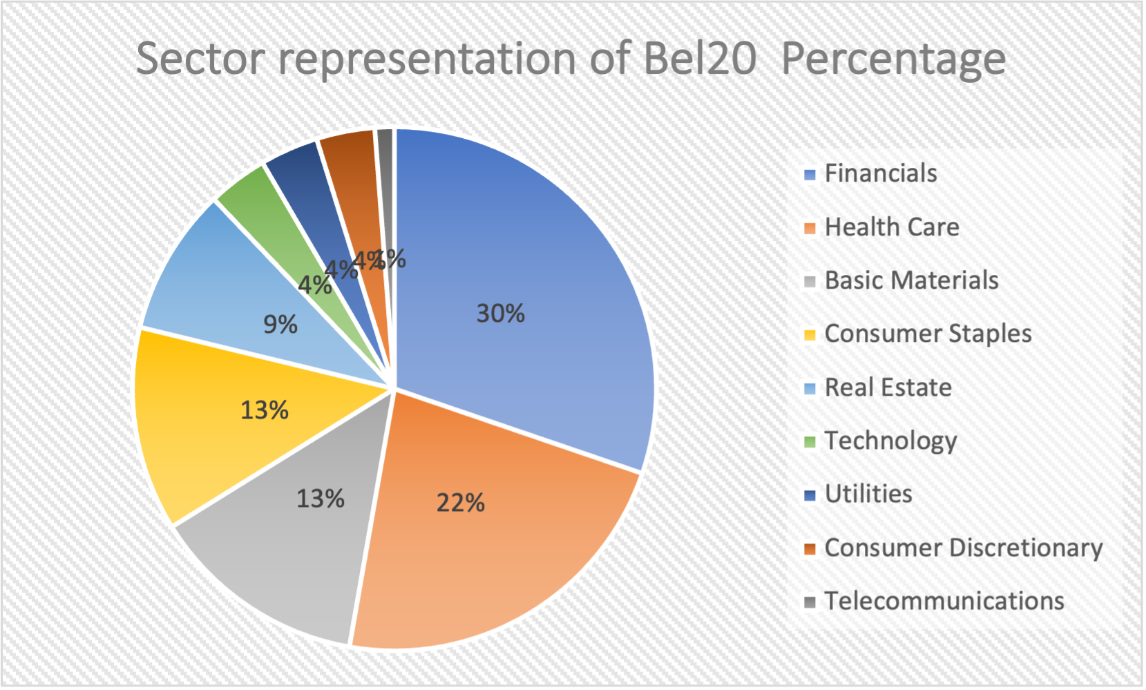
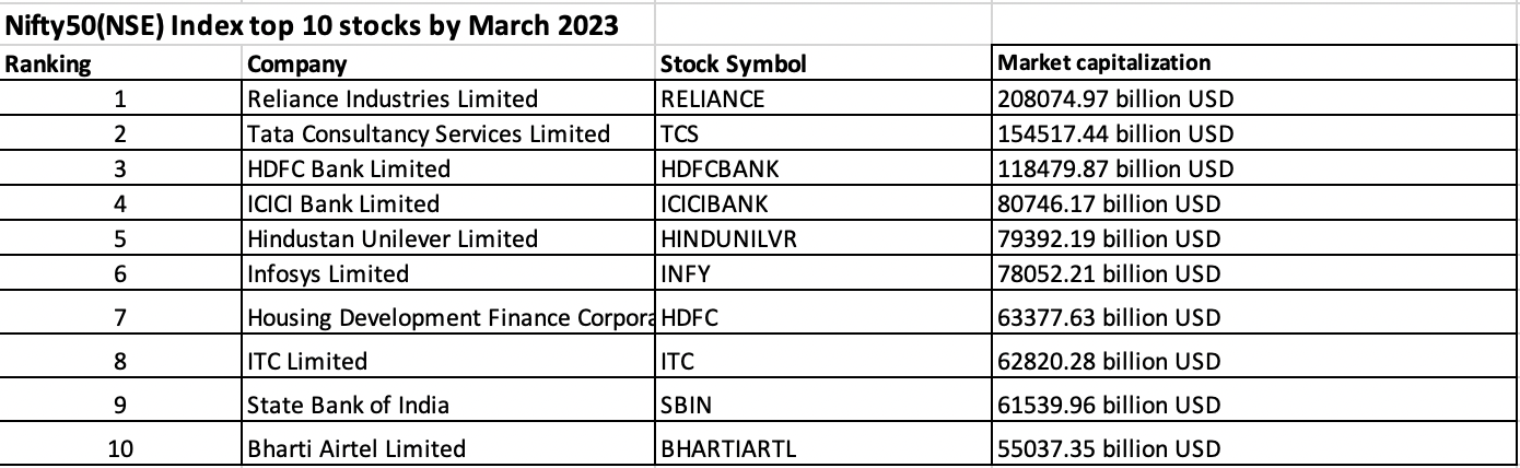
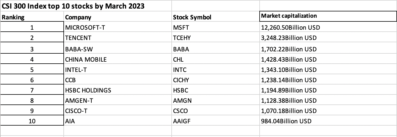
The S&P 500, or the Standard & Poor’s 500, is a renowned stock market index encompassing 500 of the largest publicly traded companies in the United States. These companies are selected based on factors like market capitalization and sector representation, making the index a diversified and reliable reflection of the U.S. stock market. It is a market capitalization-weighted index, where companies with larger market capitalization represent a greater influence on their performance. The S&P 500 is widely used as a benchmark to assess the health and trends of the U.S. economy and as a performance reference for individual stocks and investment products, including exchange-traded funds (ETF) and index funds. Its historical significance, economic indicator status, and global impact contribute to its status as a critical barometer of market conditions and overall economic health.
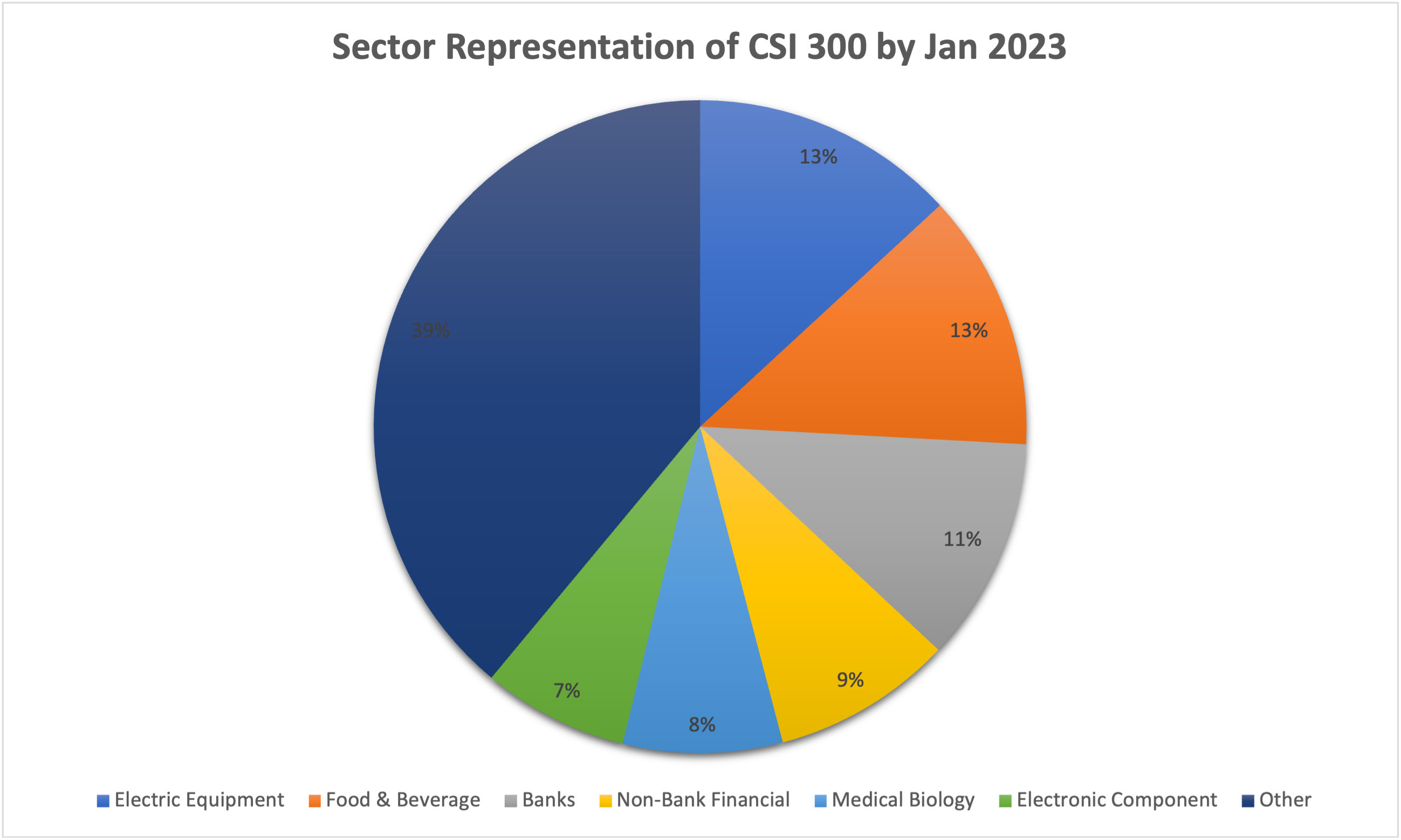
Characterized by its diversification and broad sector representation, the S&P 500 remains an essential tool for investors, policymakers, and economists to analyze market dynamics. This index’s performance, affected by economic data, geopolitical events, corporate earnings, and market sentiment, can provide valuable insights into the state of the U.S. stock market and the broader economy. Its rebalancing ensures that it remains current and representative of the ever-evolving landscape of American corporations. Overall, the S&P 500 plays a central role in shaping investment decisions and assessing the performance of the U.S. economy.
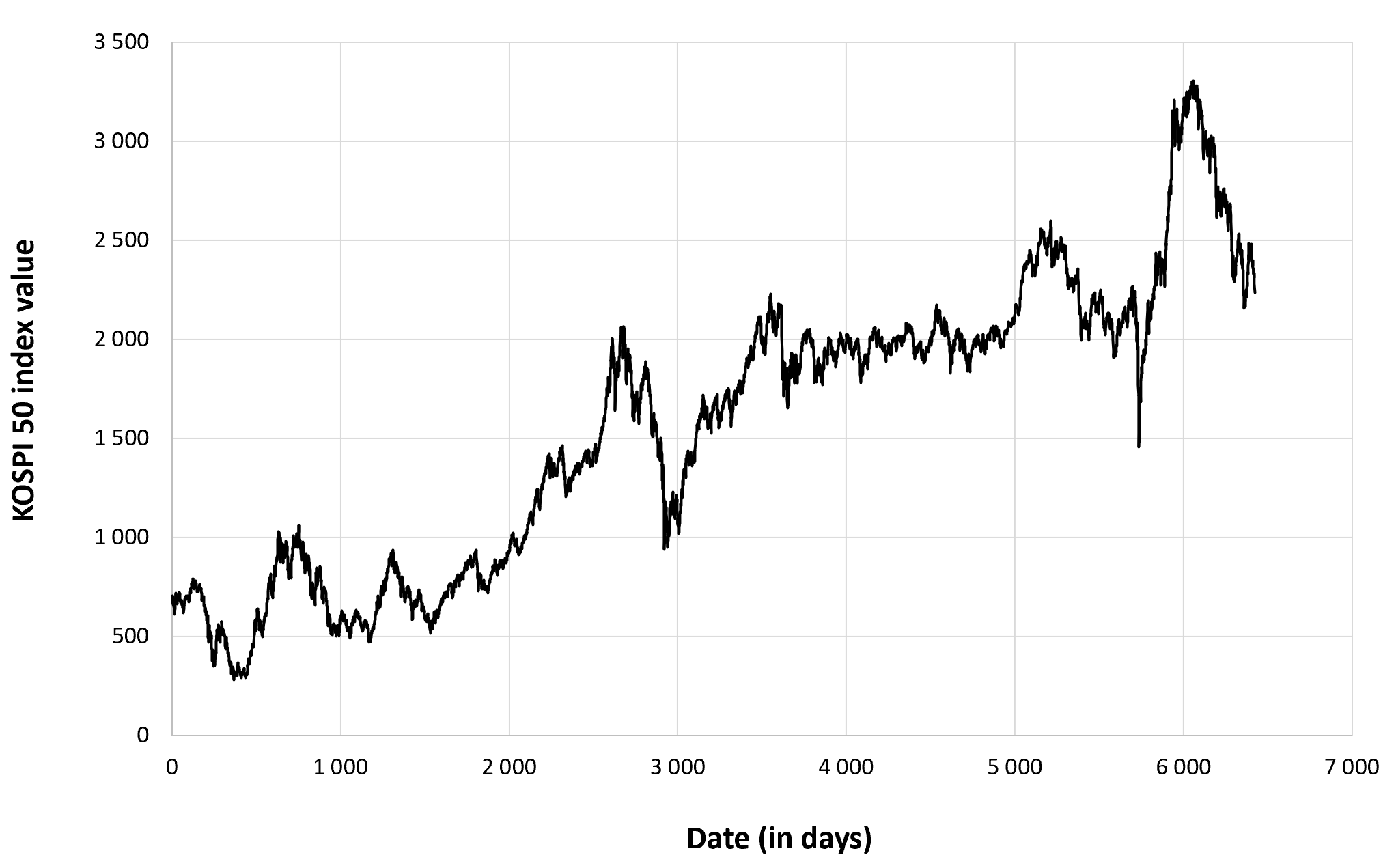
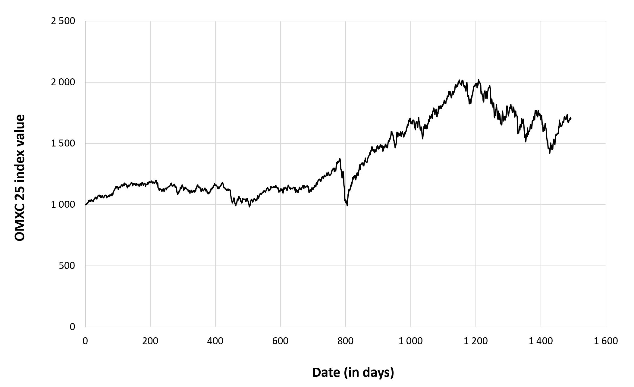
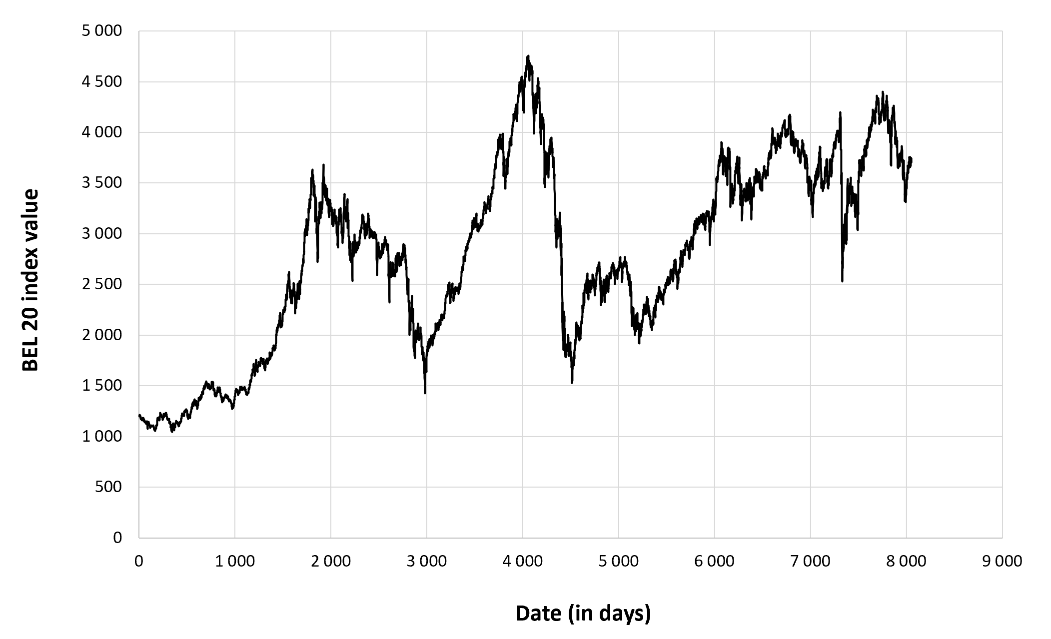
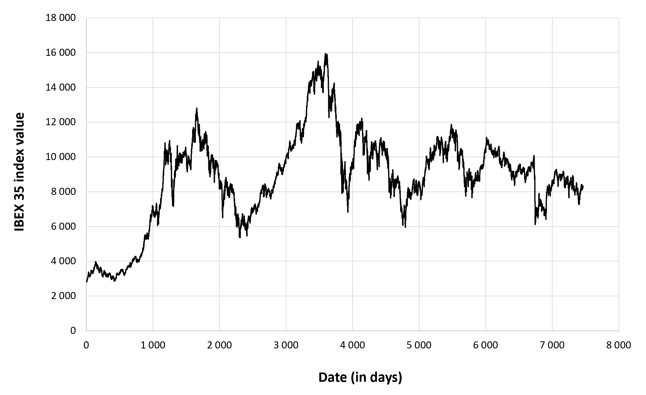
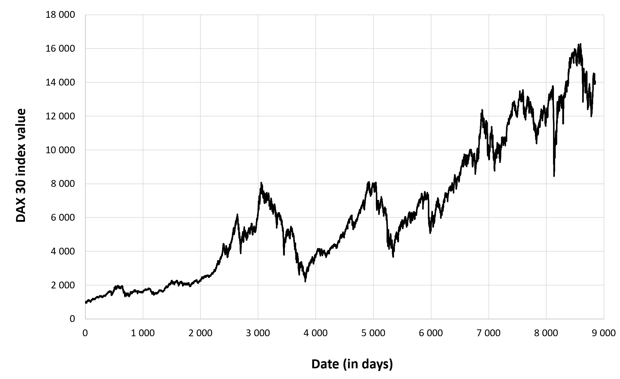
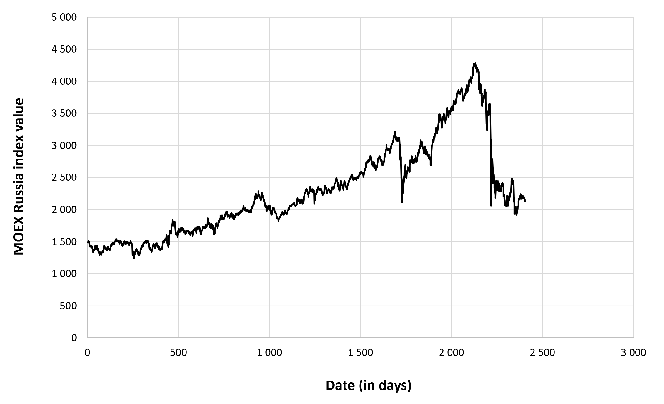
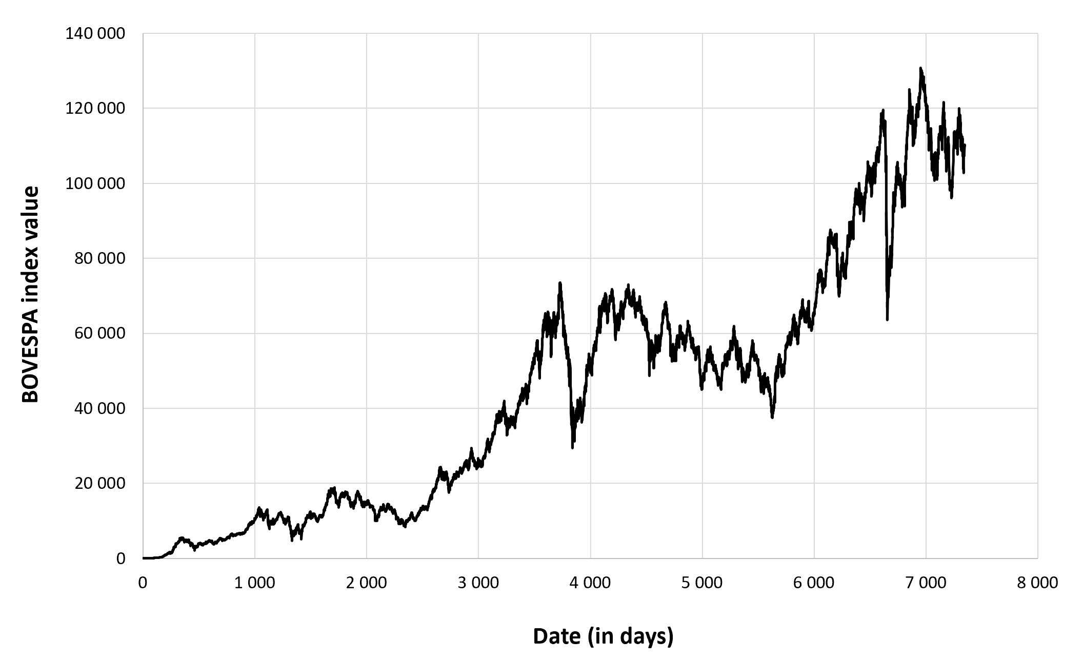
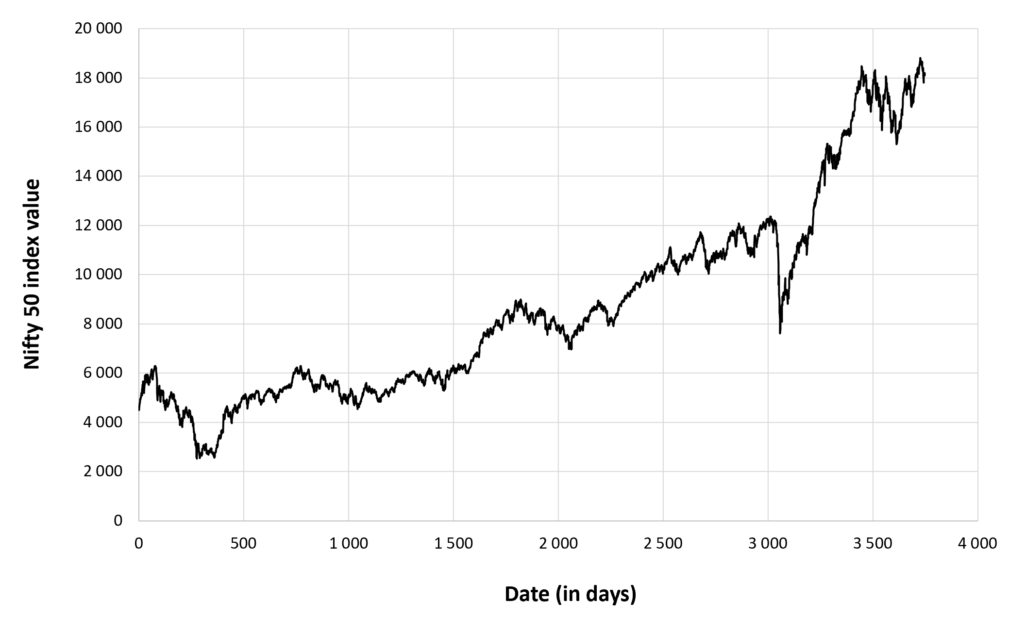
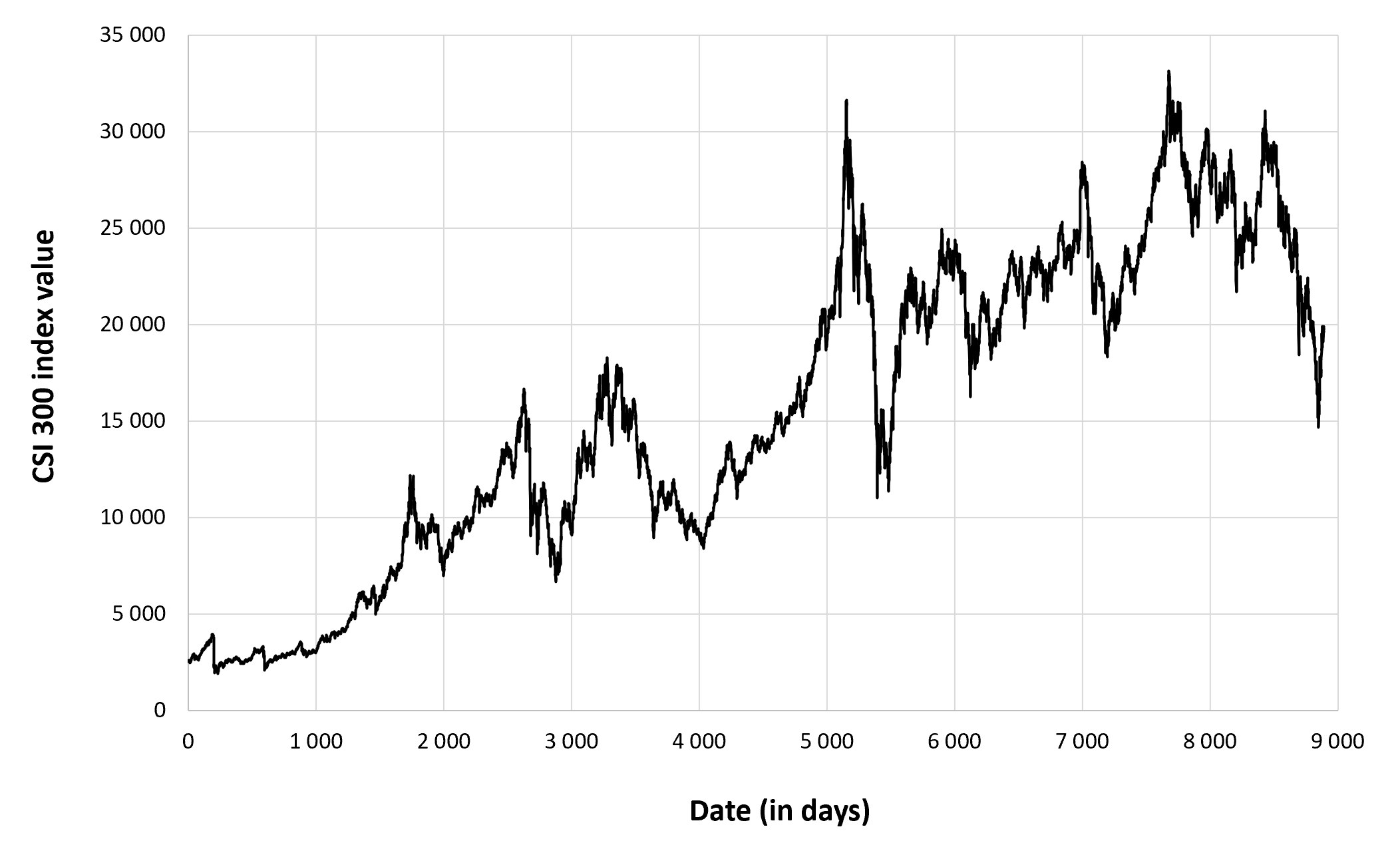
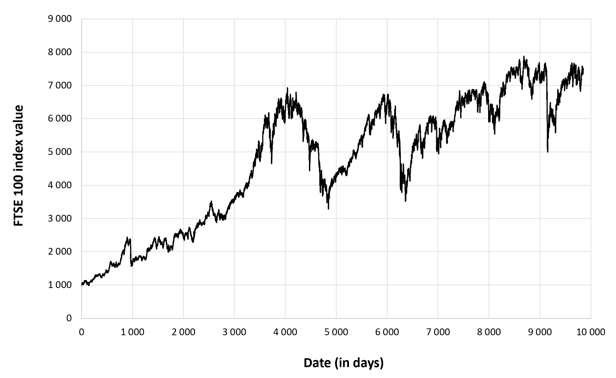
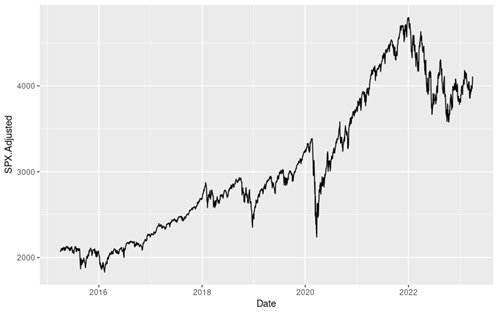
In this article, we focus on the S&P 500 index of the timeframe from April 1st, 2015, to April 1st, 2023. Here we have a line chart depicting the evolution of the index level of this period. We can observe the overall increase with remarkable drops during the covid crisis (2020) and the Russian invasion in Ukraine (2022).
Figure 1 below gives the evolution of the S&P 500 index from April 1, 2015 to April 1, 2023 on a daily basis.
Figure 1. Evolution of the S&P 500 index.
Source: computation by the author (data: Yahoo! Finance website).
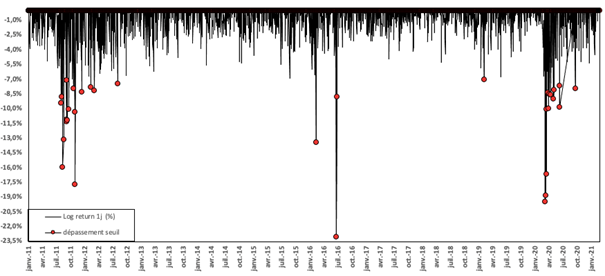
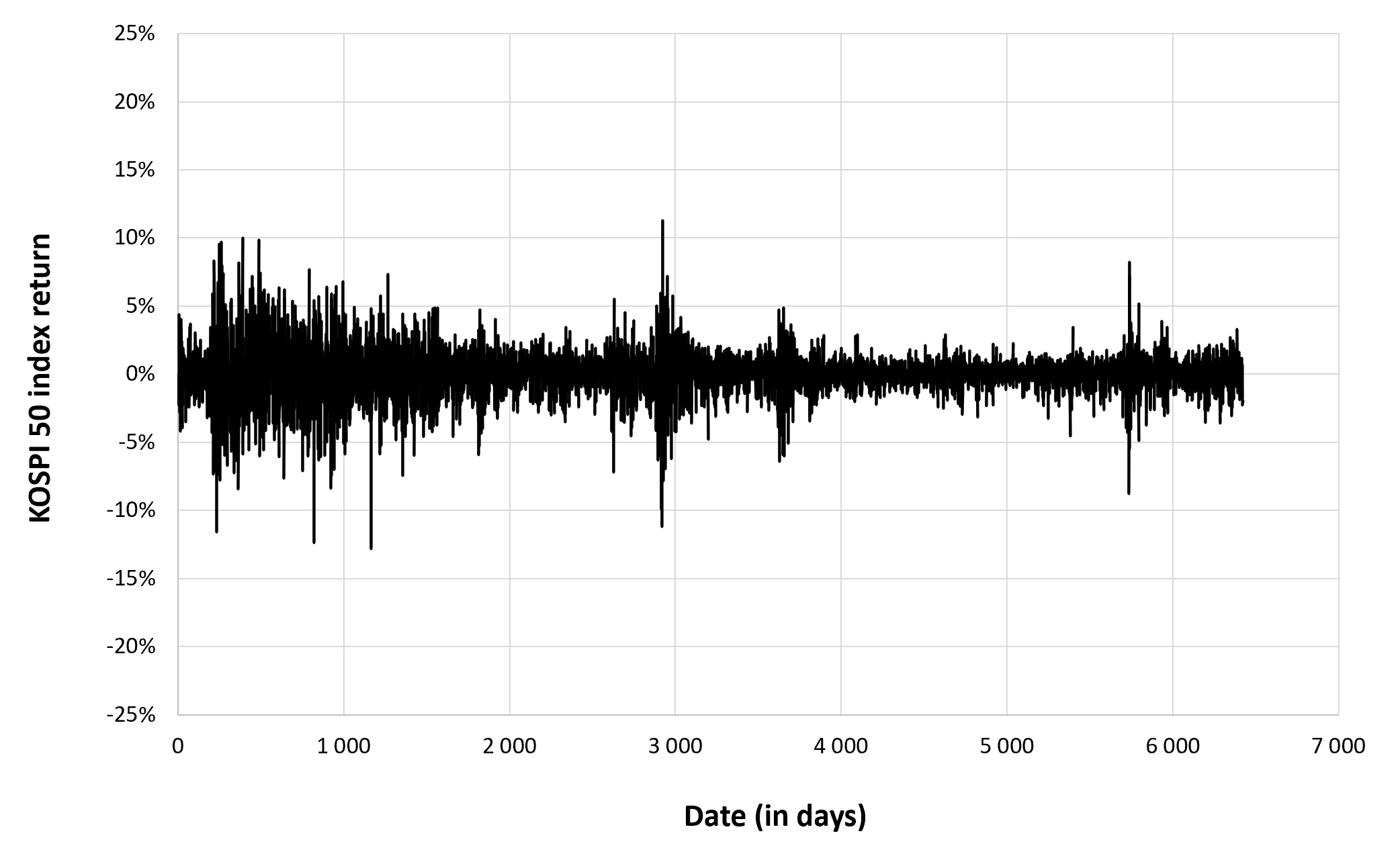
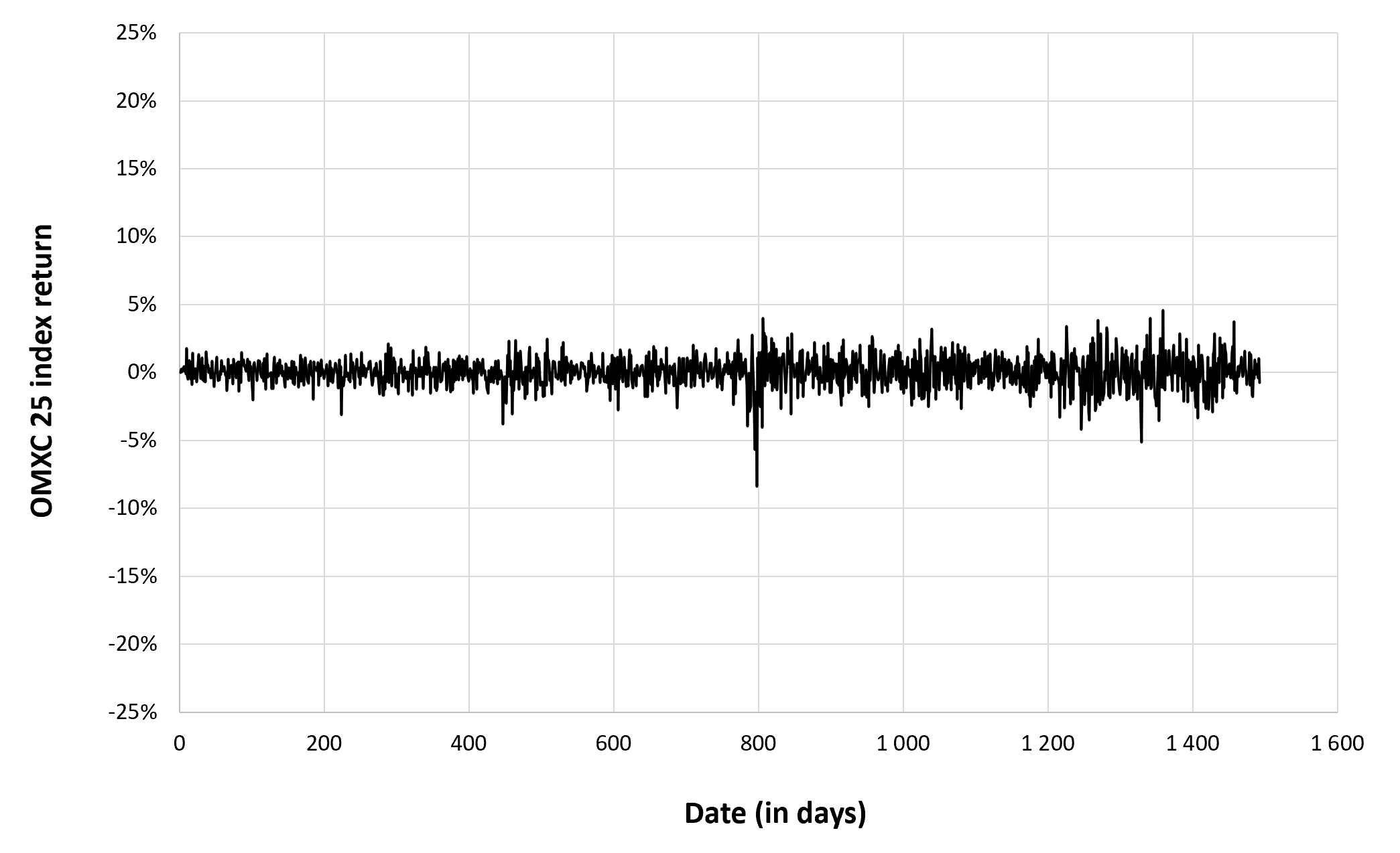
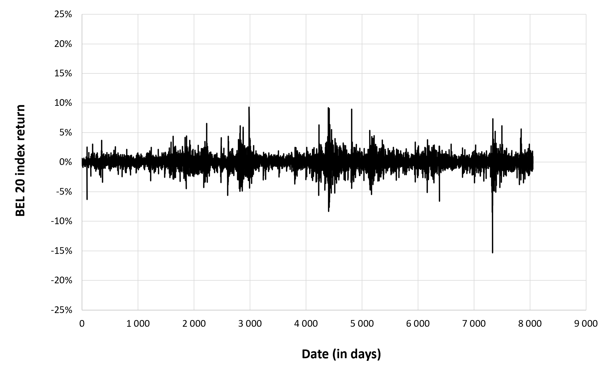
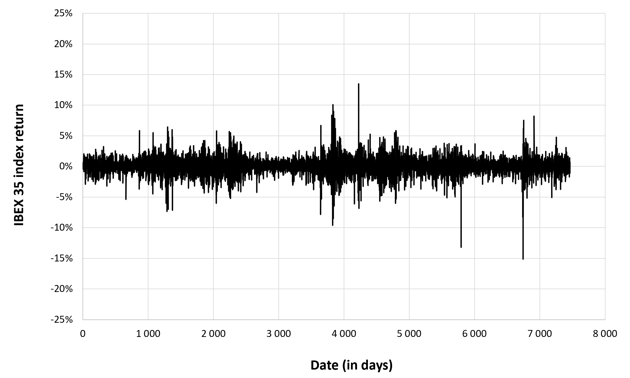
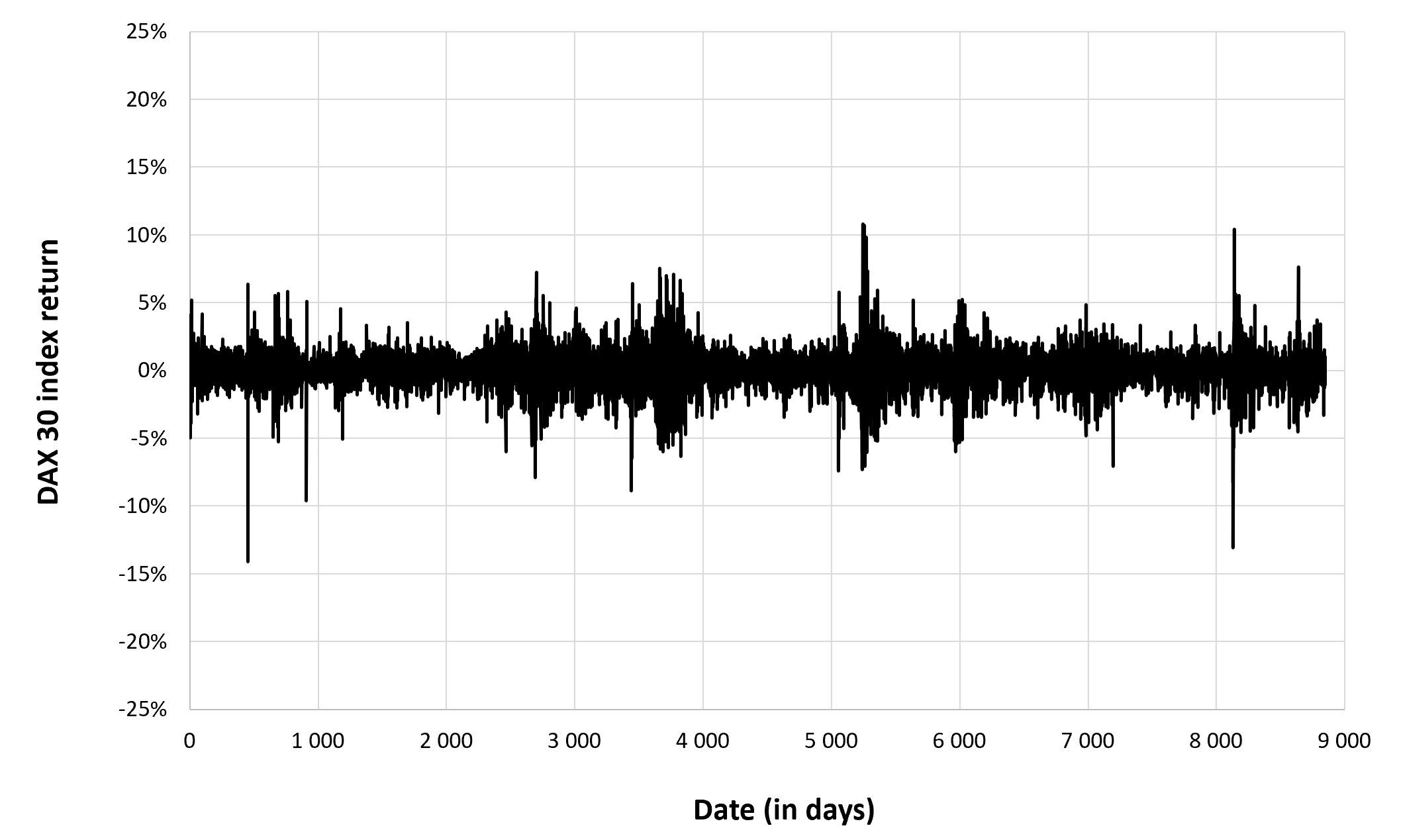
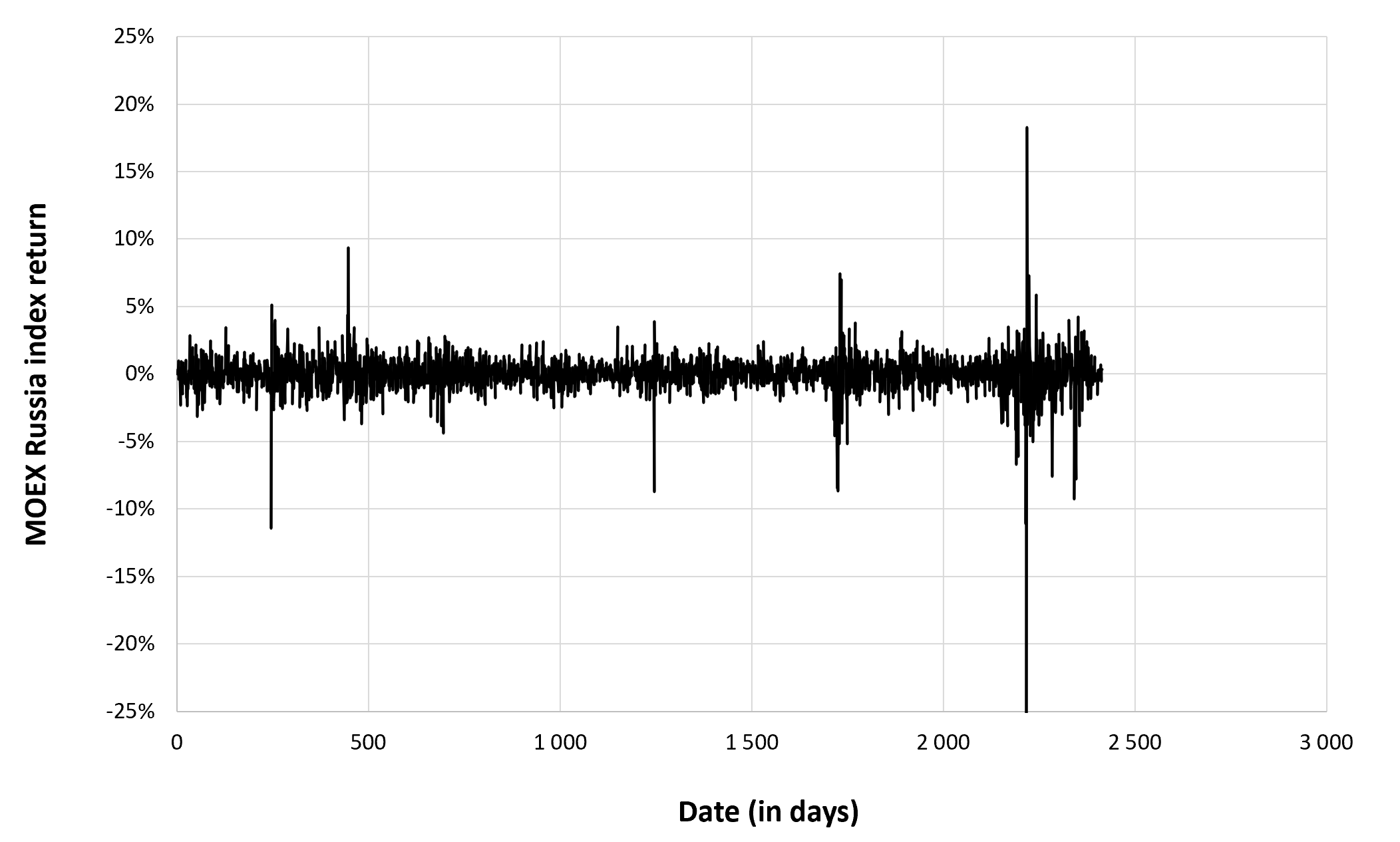
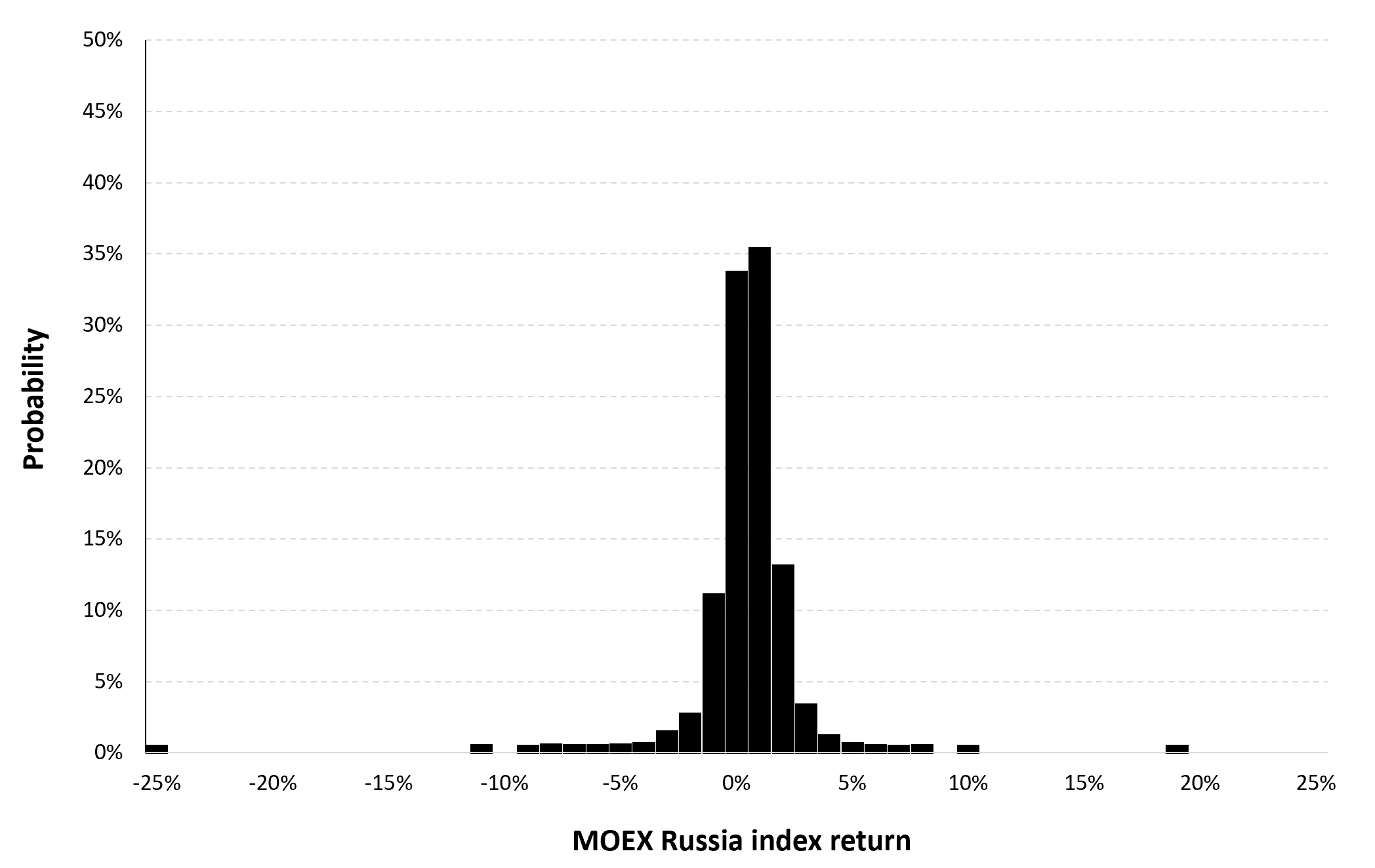
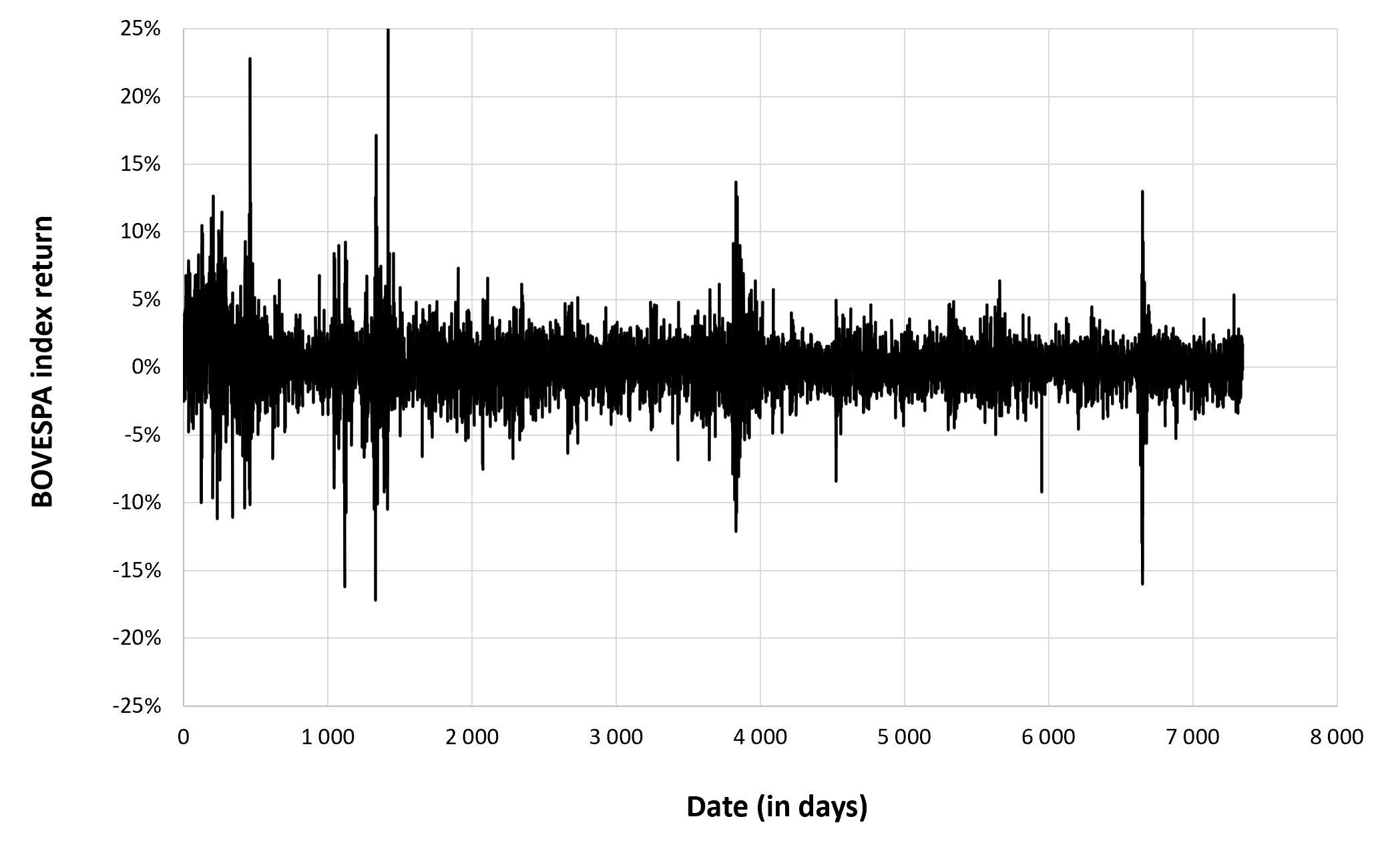
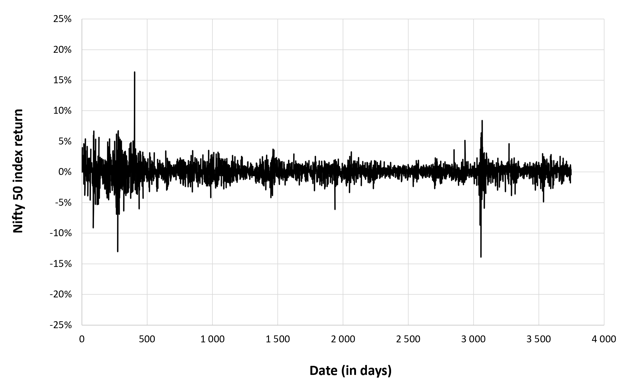
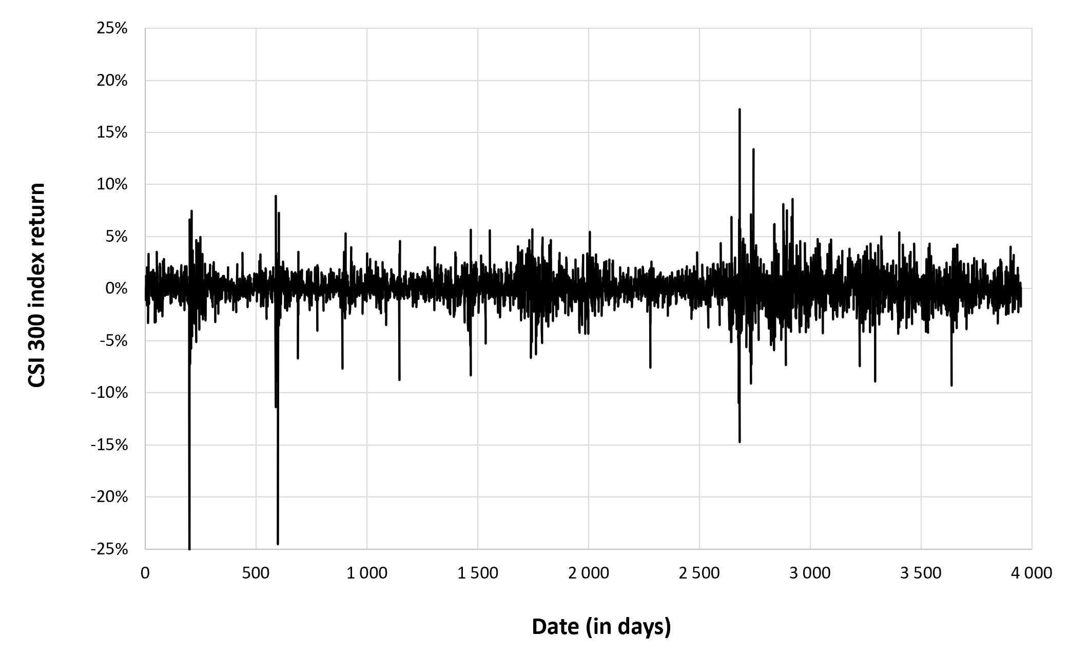
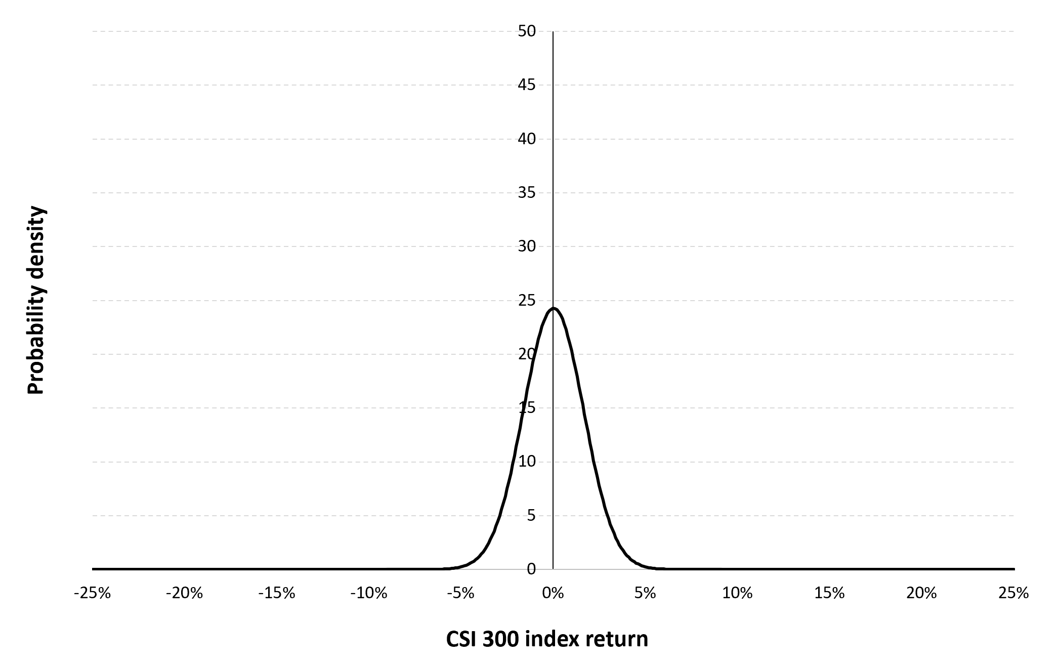
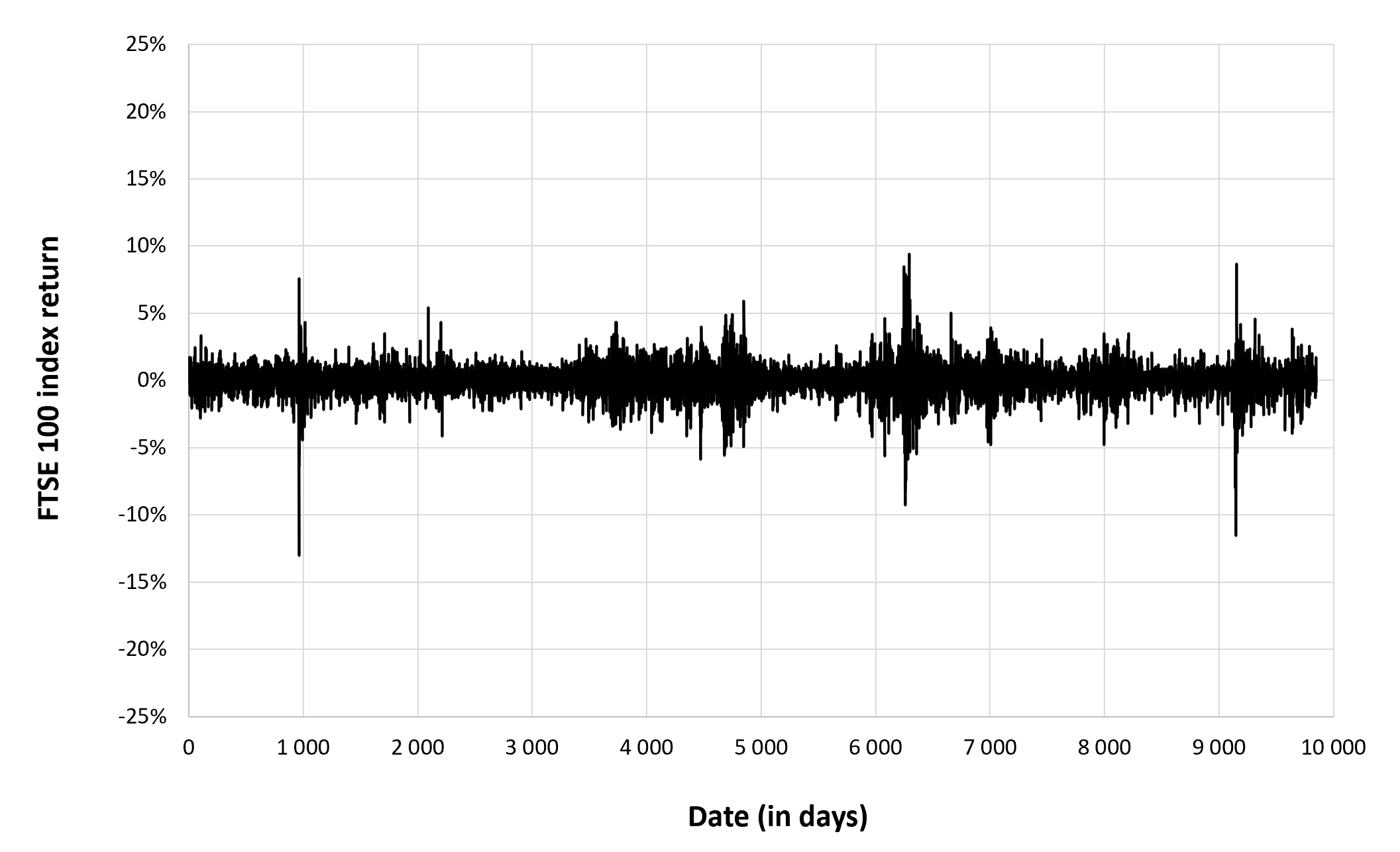
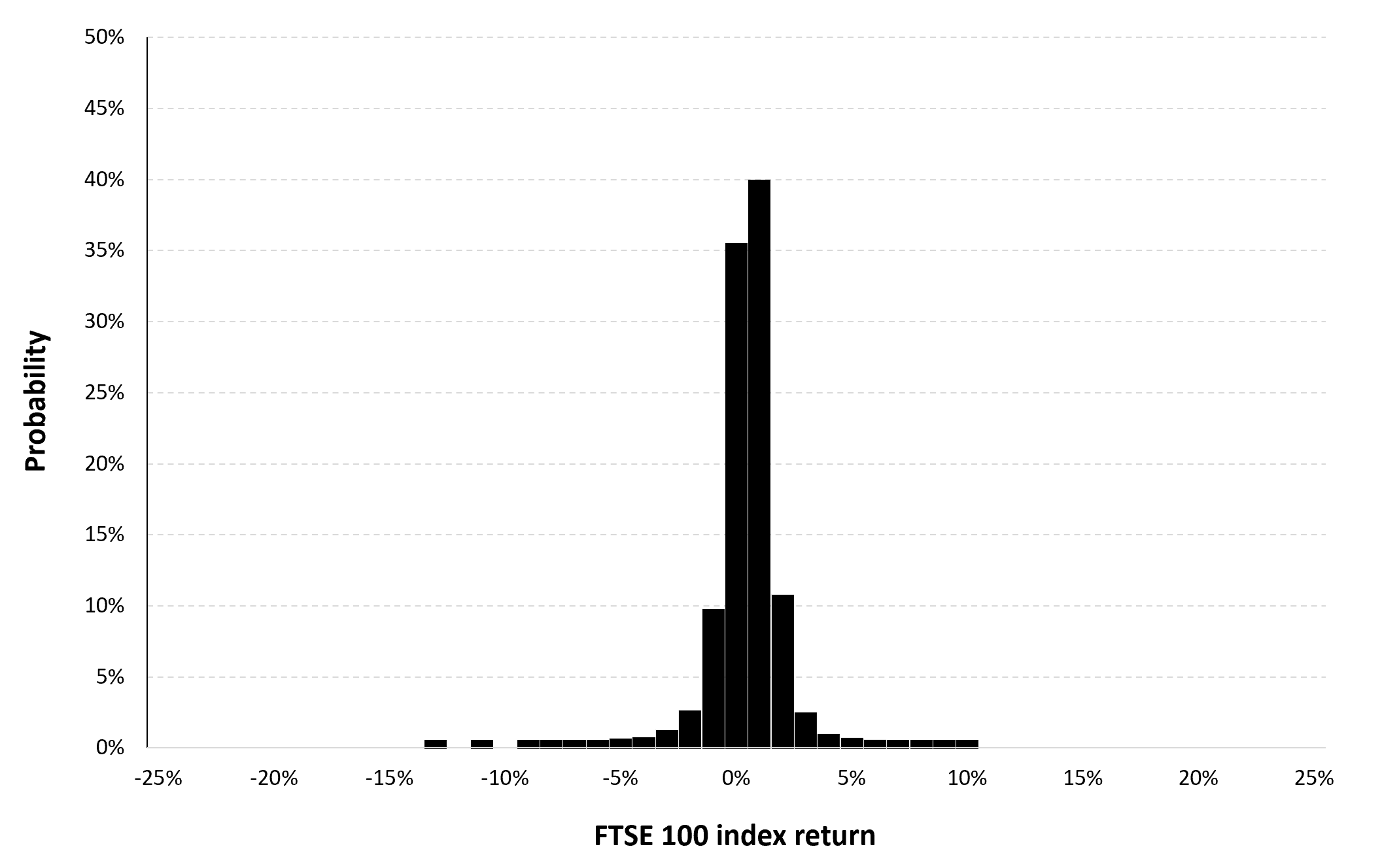
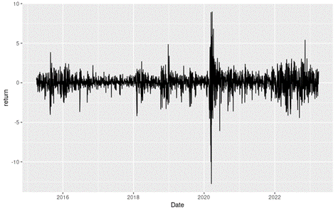
Figure 2 below gives the evolution of the daily logarithmic returns of S&P 500 index from April 1, 2015 to April 1, 2023 on a daily basis. We observe concentration of volatility reflecting large price fluctuations in both directions (up and down movements). This alternation of periods of low and high volatility is well modeled by ARCH models.
Figure 2. Evolution of the S&P 500 index logarithmic returns.
Source: computation by the author (data: Yahoo! Finance website).
Summary statistics for the S&P 500 index
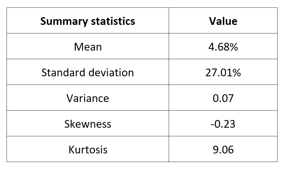
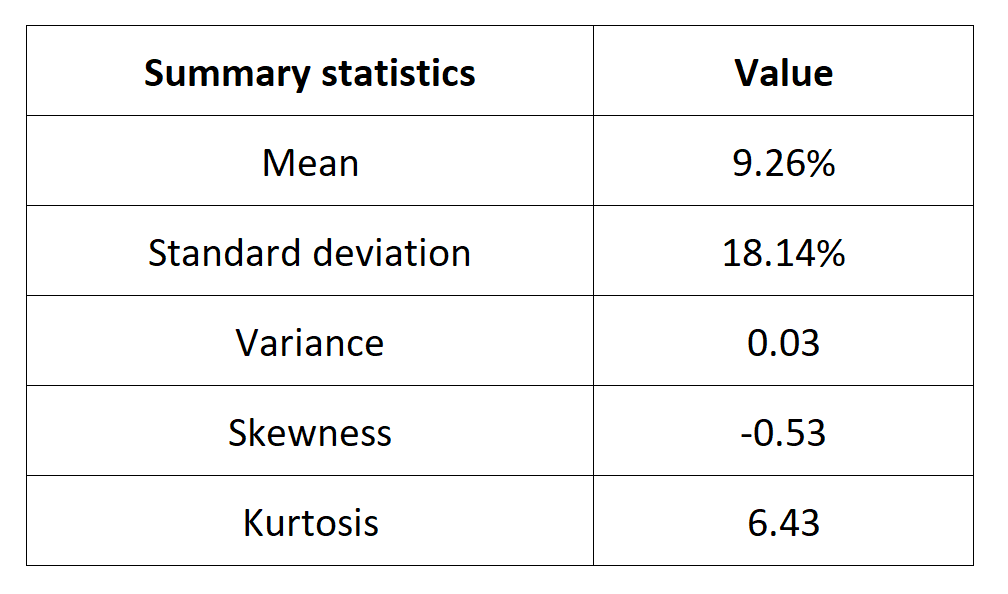
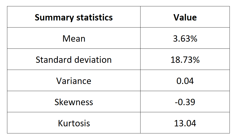
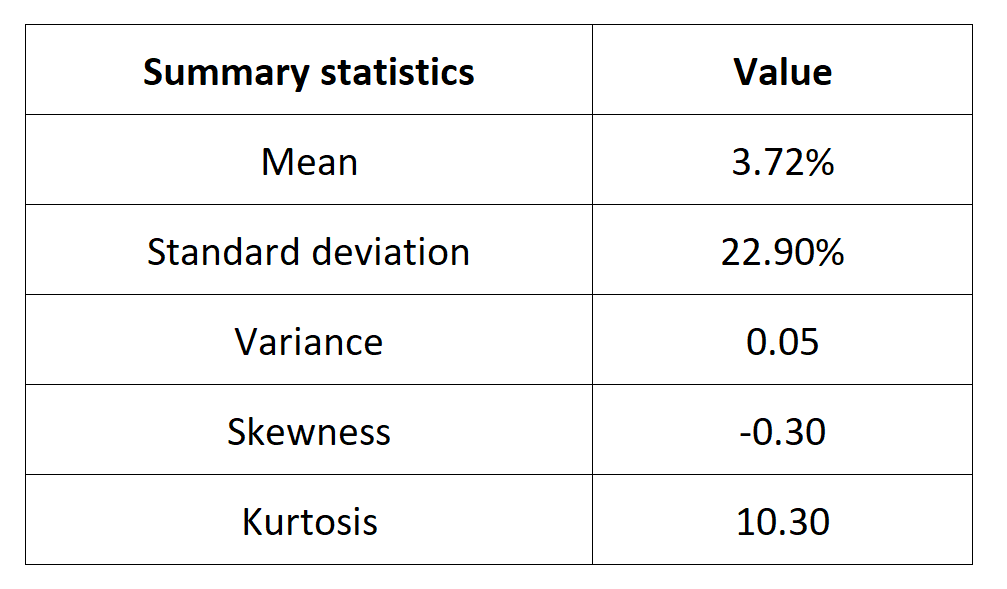
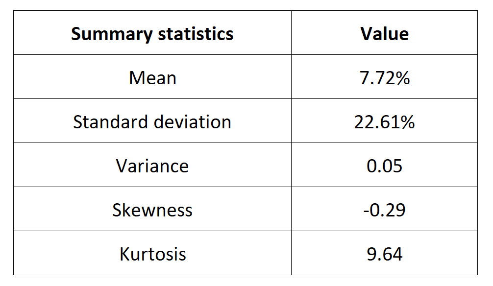
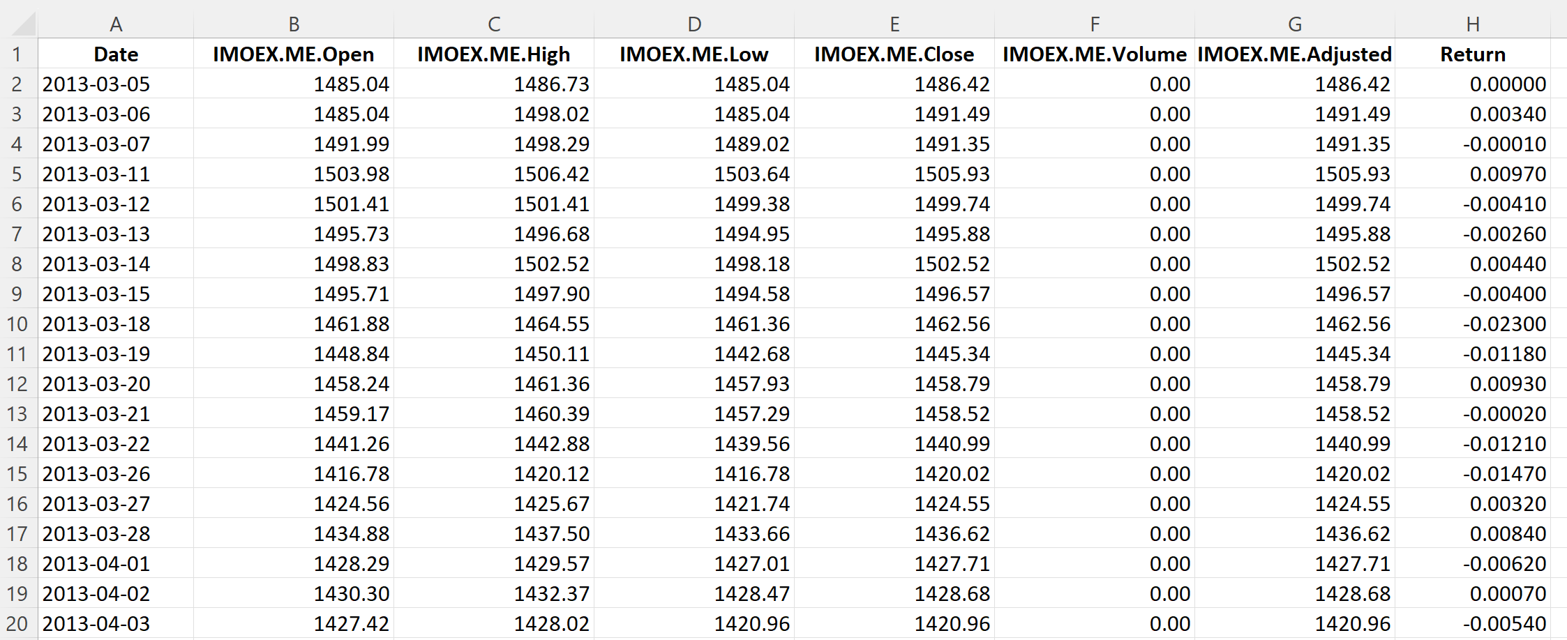
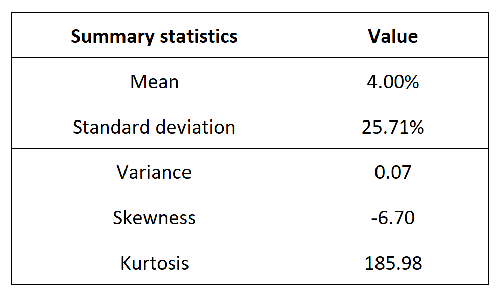
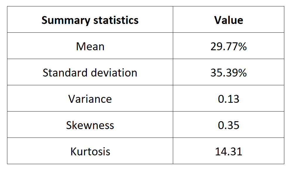
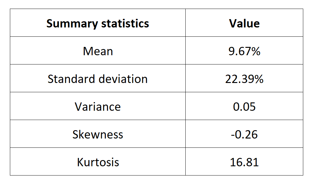
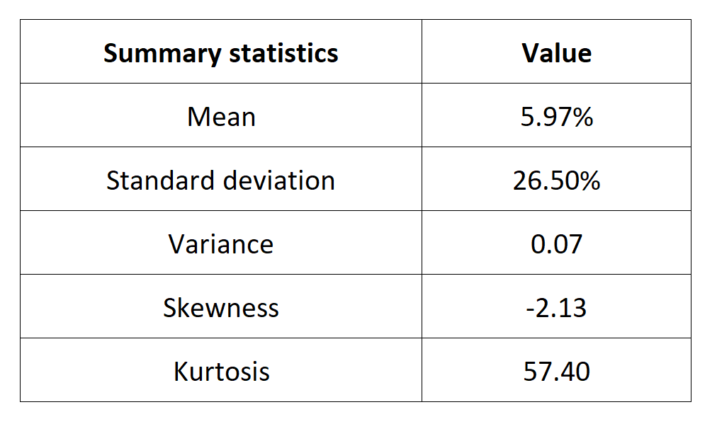
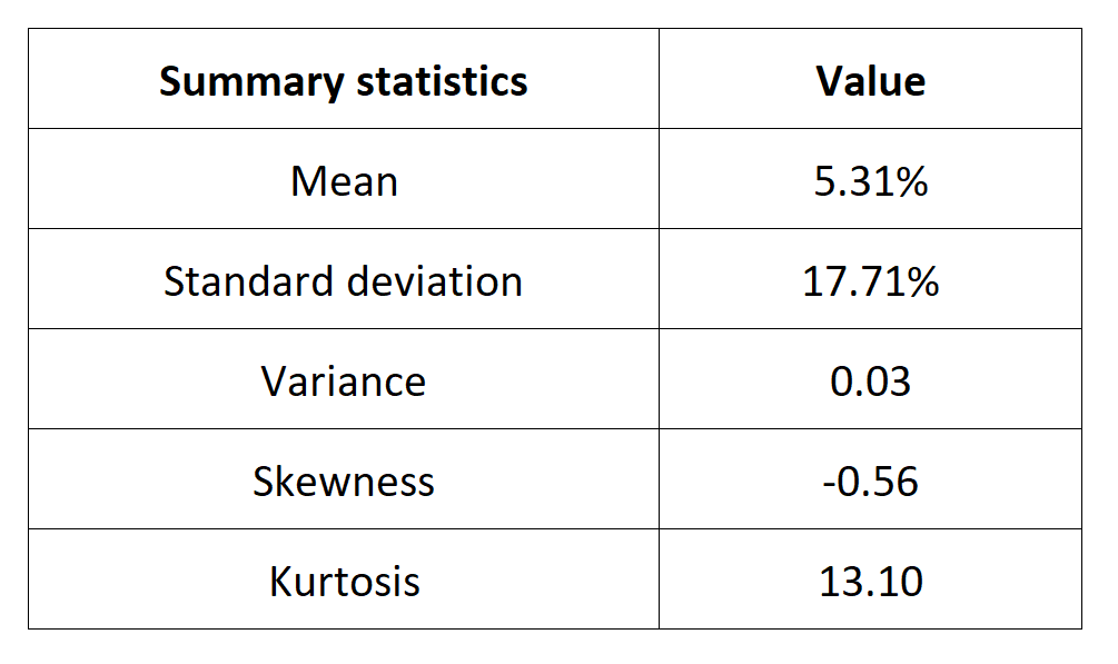
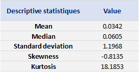
Table 1 below presents the summary statistics estimated for the S&P 500 index:
Table 1. Summary statistics for the S&P 500 index.
Source: computation by the author (data: Yahoo! Finance website).
The mean, the standard deviation / variance, the skewness, and the kurtosis refer to the first, second, third and fourth moments of statistical distribution of returns respectively. We can conclude that during this timeframe, the S&P 500 index takes on a slight upward trend, with relatively important daily deviation, negative skewness and excess of kurtosis.
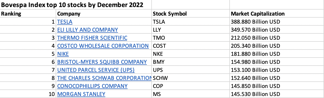
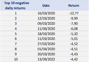
Tables 2 and 3 below present the top 10 negative daily returns and top 10 positive daily returns for the S&P 500 index over the period from April 1, 2015 to April 1, 2023.
Table 2. Top 10 negative daily returns for the S&P 500 index.
Source: computation by the author (data: Yahoo! Finance website).
Table 3. Top 10 positive daily returns for the S&P 500 index.
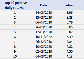
Source: computation by the author (data: Yahoo! Finance website).
Modelling of the tails
Here the tail modelling is conducted based on the Peak-over-Threshold (POT) approach which corresponds to a Generalized Pareto Distribution (GPD). Let’s recall the theoretical background of this approach.
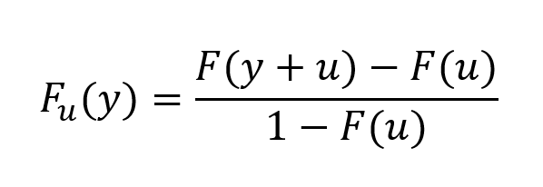
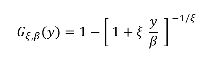
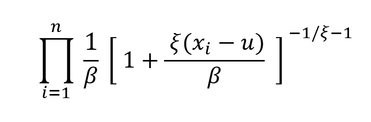
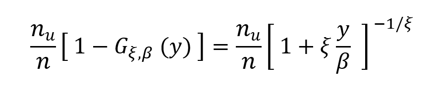
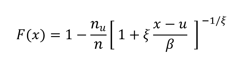
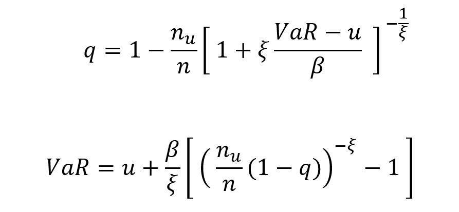
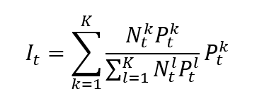
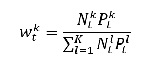
The POT approach takes into account all data entries above a designated high threshold u. The threshold exceedances could be fitted into a generalized Pareto distribution:
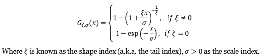
An important issue for the POT-GPD approach is the threshold selection. An optimal threshold level can be derived by calibrating the tradeoff between bias and inefficiency. There exist several approaches to address this problematic, including a Monte Carlo simulation method inspired by the work of Jansen and de Vries (1991). In this article, to fit the GPD, we use the 2.5% quantile for the modelling of the negative tail and the 97.5% quantile for that of the positive tail.
Based on the POT-GPD approach with a fixed threshold selection, we arrive at the following modelling results for the GPD for negative extreme returns (Table 4) and positive extreme returns (Table 5) for the S&P 500 index:
Table 4. Estimate of the parameters of the GPD for negative daily returns for the S&P 500 index.
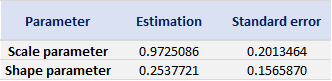
Source: computation by the author (data: Yahoo! Finance website).
Table 5. Estimate of the parameters of the GPD for positive daily returns for the S&P 500 index.
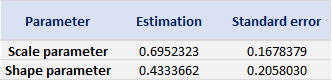
Source: computation by the author (data: Yahoo! Finance website).
Figure 3. GPD for the left tail of the S&P 500 index returns.
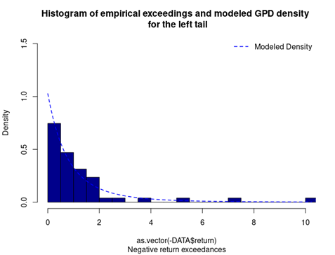
Source: computation by the author (data: Yahoo! Finance website).
Figure 4. GPD for the right tail of the S&P 500 index returns.
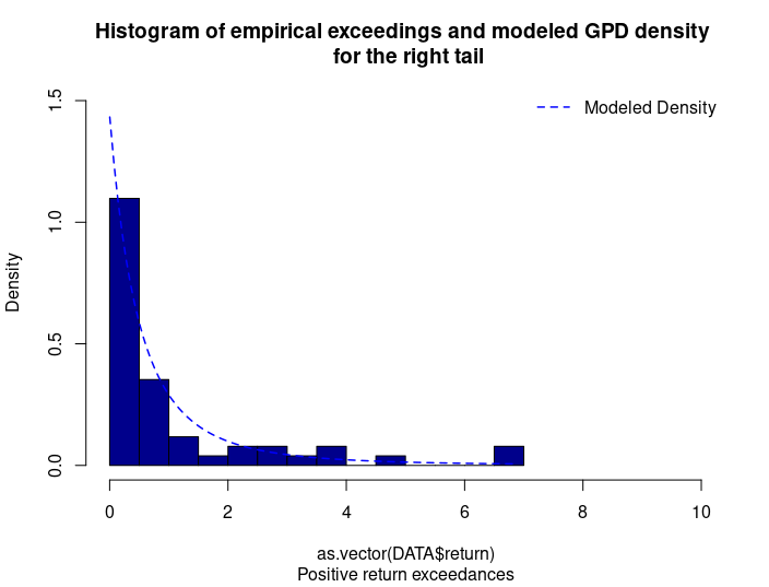
Source: computation by the author (data: Yahoo! Finance website).
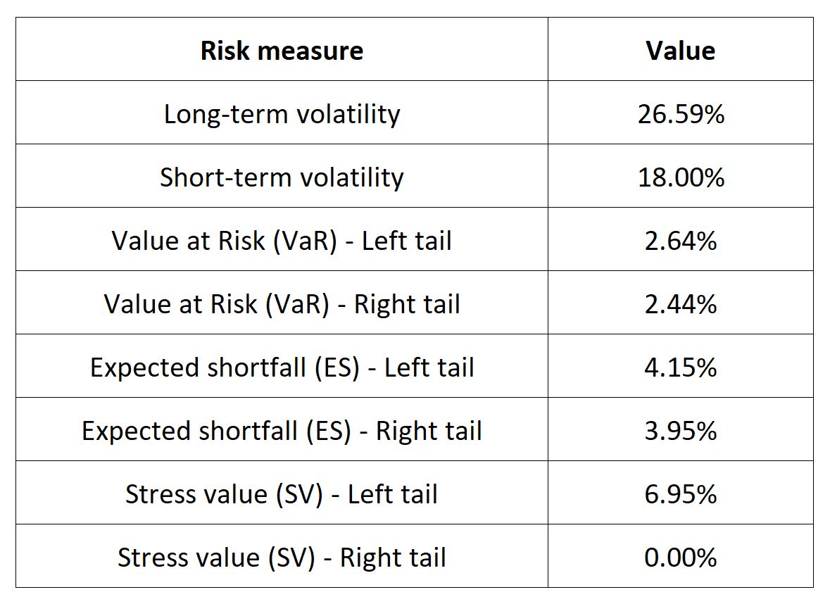
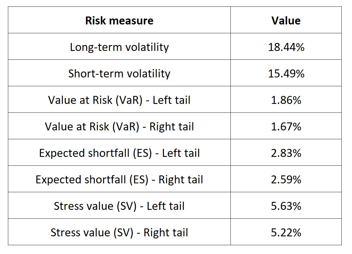
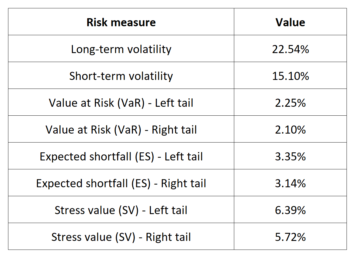
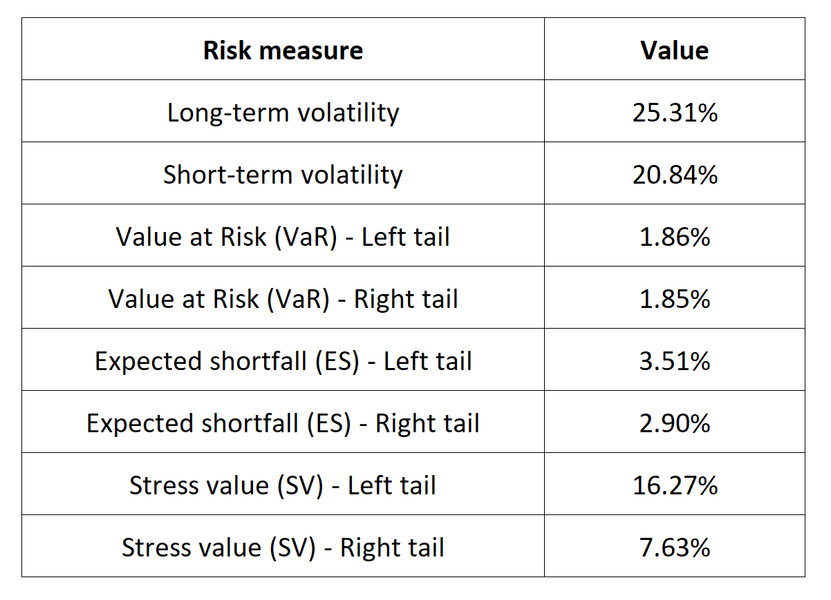
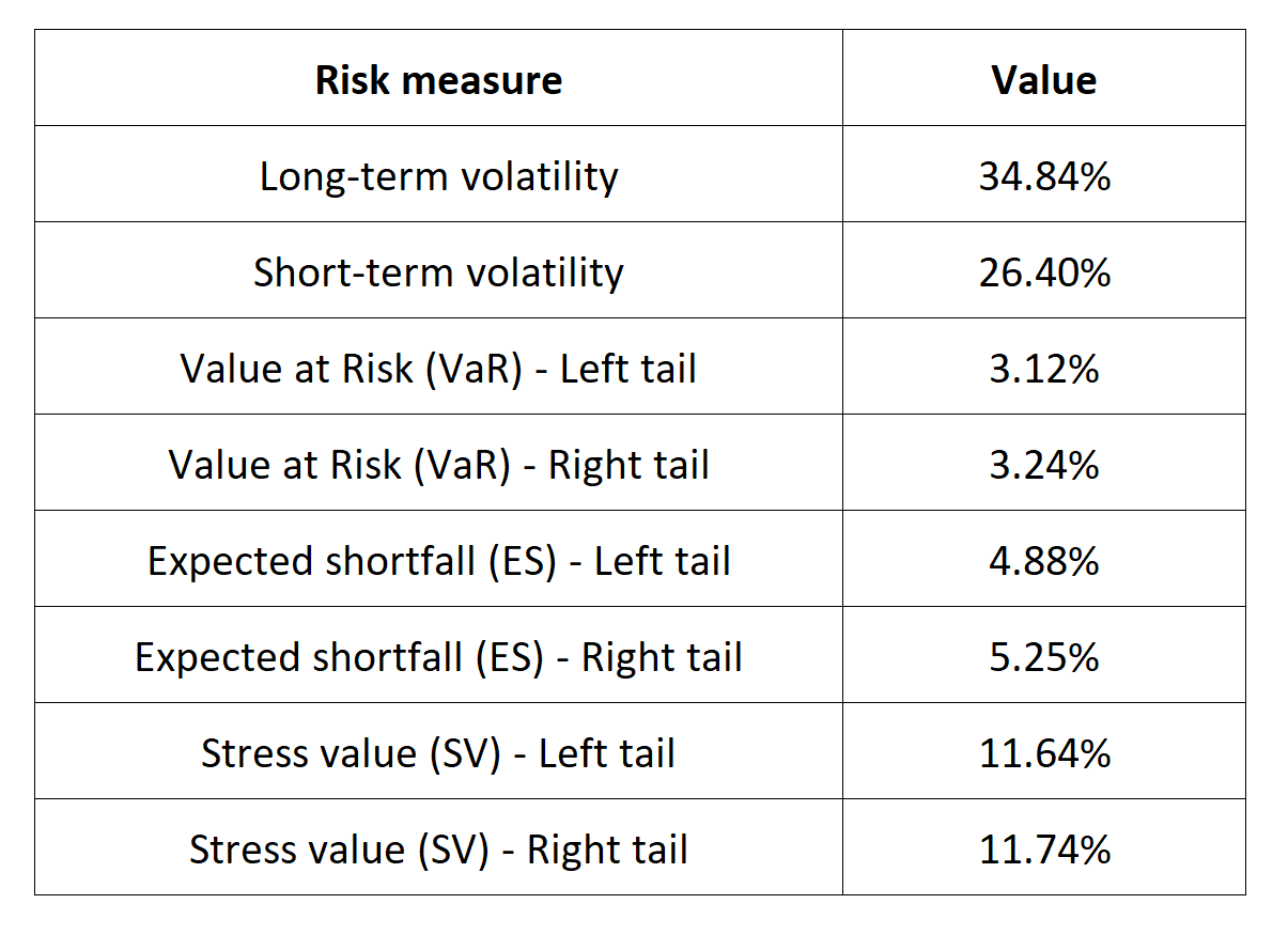
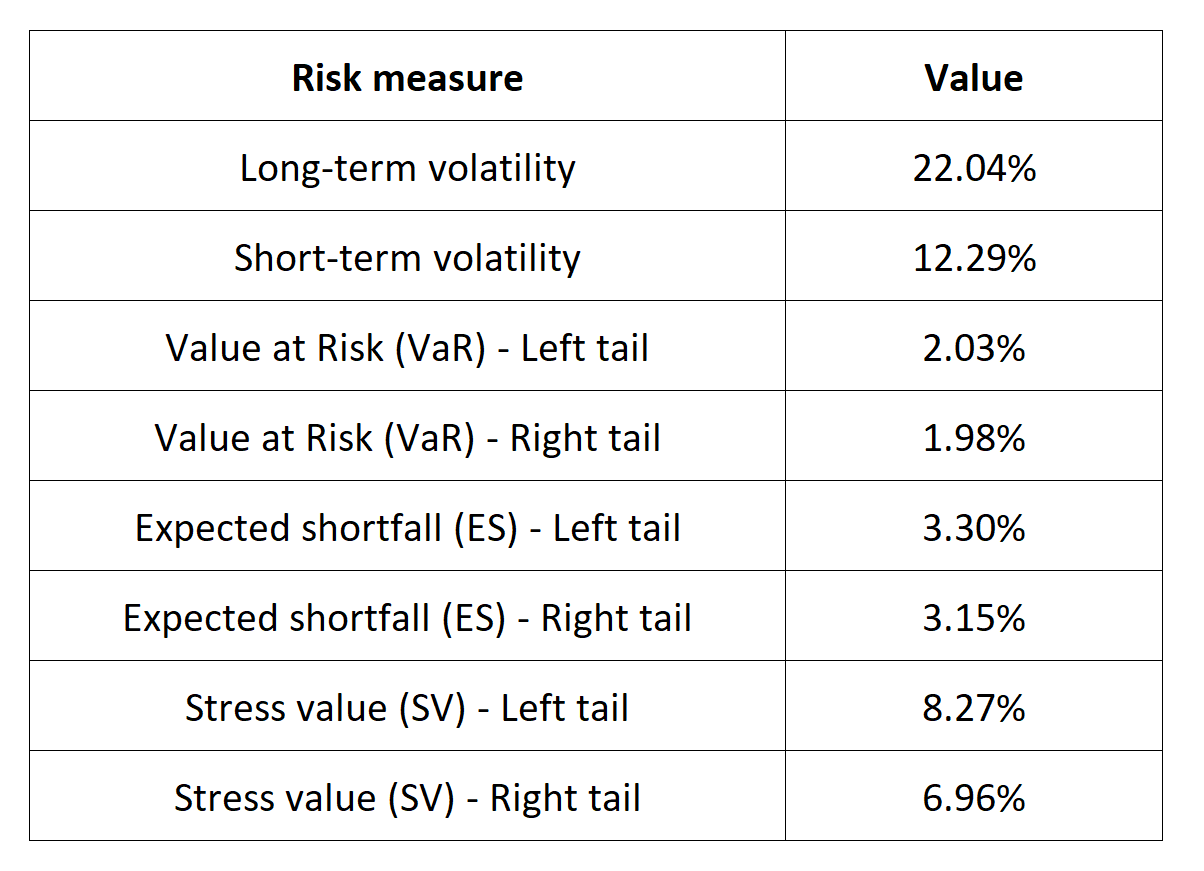
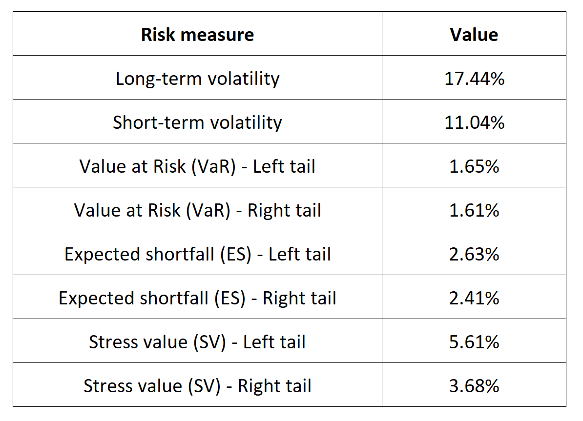
Applications in risk management
Extreme Value Theory (EVT) as a statistical approach is used to analyze the tails of a distribution, focusing on extreme events or rare occurrences. EVT can be applied to various risk management techniques, including Value at Risk (VaR), Expected Shortfall (ES), and stress testing, to provide a more comprehensive understanding of extreme risks in financial markets.
Why should I be interested in this post?
Extreme Value Theory is a useful tool to model the tails of the evolution of a financial instrument. In the ever-evolving landscape of financial markets, being able to grasp the concept of EVT presents a unique edge to students who aspire to become an investment or risk manager. It not only provides a deeper insight into the dynamics of equity markets but also equips them with a practical skill set essential for risk analysis. By exploring how EVT refines risk measures like Value at Risk (VaR) and Expected Shortfall (ES) and its role in stress testing, students gain a valuable perspective on how financial institutions navigate during extreme events. In a world where financial crises and market volatility are recurrent, this post opens the door to a powerful analytical framework that contributes to informed decisions and financial stability.
Download R file to model extreme behavior of the index
You can find below an R file (file with txt format) to study extreme returns and model the distribution tails for the S&P 500 index.

Related posts on the SimTrade blog
About financial indexes
▶ Nithisha CHALLA Financial indexes
▶ Nithisha CHALLA Calculation of financial indexes
▶ Nithisha CHALLA The S&P 500 index
About portfolio management
▶ Youssef LOURAOUI Portfolio
▶ Jayati WALIA Returns
About statistics
▶ Shengyu ZHENG Moments de la distribution
▶ Shengyu ZHENG Mesures de risques
▶ Shengyu ZHENG Extreme Value Theory: the Block-Maxima approach and the Peak-Over-Threshold approach
▶ Gabriel FILJA Application de la théorie des valeurs extrêmes en finance de marchés
Useful resources
Academic resources
Embrechts P., C. Klüppelberg and T. Mikosch (1997) Modelling Extremal Events for Insurance and Finance Springer-Verlag.
Embrechts P., R. Frey, McNeil A.J. (2022) Quantitative Risk Management Princeton University Press.
Gumbel, E. J. (1958) Statistics of extremes New York: Columbia University Press.
Longin F. (2016) Extreme events in finance: a handbook of extreme value theory and its applications Wiley Editions.
Other resources
Chan S. Statistical tools for extreme value analysis
Rieder H. E. (2014) Extreme Value Theory: A primer (slides).
About the author
The article was written in October 2023 by Shengyu ZHENG (ESSEC Business School, Grande Ecole Program – Master in Management, 2020-2024).