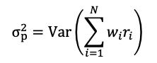
The regulation of cryptocurrencies: what are we talking about?

In this article, Hugo MEYER (ESSEC Business School, Master in Strategy & Management of International Business (SMIB), 2020-2021) presents the regulation of cryptocurrencies.
Introduction
The first cryptocurrency – Bitcoin – launched in 2008 by Satoshi Nakamoto had for ambition to “break the rules and change the world”.
Thirteen years later, cryptocurrency represents a 2$ trillion market, with an increasing institutional presence, from crypto hedge funds to large banks. Behind this bewildering evolution, public authorities lagged behind, slowly empowering with feverish regulation actions.
The lack of regulation in this burgeoning area has created an opening for boundless fraud and money laundering, forcing some countries to get to grips with the cryptocurrency’s pitfalls.
What are cryptocurrencies?
Cryptocurrencies are at the edge of revolutionizing the way we’ve been trading since thousands of years. By definition, a cryptocurrency is an encrypted, digital, and decentralized medium of exchange that allows two parties that could be located everywhere on the globe to transfer funds directly, without relying on any trusted third party.
Instead of being secured by public institutions and/or companies, these transfers are carried out on the Blockchain which is a “digital database or ledger containing information that can be simultaneously used and shared within a large decentralized, publicly accessible network”.
Example: To make it simple, let’s say that A wants to send money to B. This transaction is included in a ‘block’. This block is broadcasted to every member in the network, and then validated or not by them. Once validated, the block is added to the chain, triggering the money to move from A to B.
Figure 1. Process of transaction with the blockchain
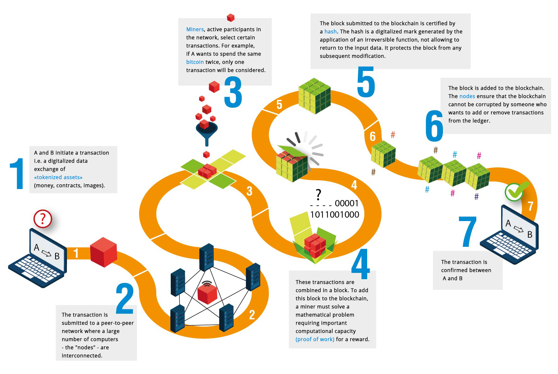
Source: Institut des actuaires.
This distributed network provides an indelible and transparent record of transactions as the chain cannot be counterfeited. If someone tried to change any information contained in one block, the different parties of the network would not approve the transaction as they could check the whole history of the blockchain and compare it to the new one.
Thus, many cryptocurrencies such as Bitcoin, Ethereum and Monero rely on public blockchains to allow transactions in complete security and transparency.
“I do think Bitcoin is the first money that has the potential to do something like change the world” – Peter THIEL.
What is the regulation about?
By definition, regulation tally with the act of controlling something, or enacting an official rule. What does it imply for cryptocurrencies?
A cryptocurrency is entirely defined by its creator, that must foremost determine its characteristics. This creation process is divided into three steps:
- Pick or create its blockchain platform
- Choose a consensus algorithm
- Design the blockchain architecture.
His creator defines the rules around it, while the ecosystem built accordingly to these rules regulate it and make it functional. Once the crypto is launched, it is impossible to modify its architecture and the rules. In this way, a cryptocurrency cannot be regulated, even by his founder. Thus, authorities do not have any grip with cryptocurrencies in themselves. They are auto-regulated by their initial algorithms, and nothing else.
Thereby, what are we talking about when dealing with the regulation of cryptocurrency?
Cryptocurrencies are mainly exchanged through platforms called “exchanges” such as Coinbase, Binance or eToroX. The first existing regulation framework is the accessibility to these platforms. For most of them, requirements like providing its identity are requested, following the Know Your Customer (KYC) compliance.
Secondly, the regulatory framework for these platforms depends on where they are based. Each country has a different approach of cryptocurrency, meaning that the regulation can be different in any of them.
For example, cryptocurrency exchanges are legal in the United States and fall under the regulatory scope of the Bank Secrecy Act (BSA). Therefore, exchanges service providers must register with FinCEN, implement an anti-money laundering (AML) and combating the financing of terrorism (CFT) program, maintain appropriate records, and submit reports to the authorities. It does not mean their trading activities are regulated.
These requirements permit exchanges to operate as licensed Money Service Businesses (MSBs), leading regulators to focus on anti-money laundering (AML) and due diligence measures, but not trading (and all the aspects of market manipulation).
Given the lack of significant regulatory oversight of actual trading activity, it is not surprising to see many cryptocurrency exchanges carry out questionable activities, such as offering leverage to their clients and wash trading, during times of market instability. But these are not the only problems raised by the lack of regulation.
Why should exchanges be more regulated?
The blockchain is a recent technology, understood by a few. As regulation always comes after innovation, the crypto market has been sidelined by public authorities for many years. The question of regulating it has recently appeared in response to the many downsides incurred to cryptos.
Customer protection
When investing in cryptocurrencies, the customer is lacking protection. An investor could be facing fake websites, hacking, and platform bankrupts without any legal recourse to recover his money. These situations could never happen in a traditional investment as it is institutionally regulated. To become more secure, exchanges must follow the example of itBit, an US-based exchange oversighted by the New York Department of Financial Services (DFS) and registered as a bank.
Illegal Financial flows & crime
Cryptocurrency can be used for illicit transactions and for laundering criminal proceeds that may or may not have started as cryptocurrency. These illicit transactions occur on the dark web, including the purchase/sale of illicit drugs and debit and credit card information. According to a study published in 2019 by Oxford Academics, 76$ billion of illegal activity per year involve bitcoin, which represents half of total Bitcoin transactions.
Cryptos can also be used for ransomware attacks, like the one that shut down the Colonial Pipeline in May 2021. This attack was one of many others high-profile instances of hackers seeking Bitcoin ransoms, that should tend to multiply in the upcoming years.
Price stability
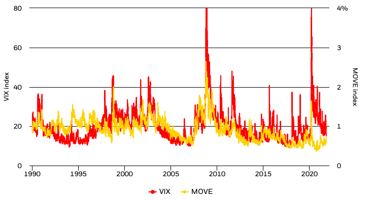
Blockchain technology has increasingly become a speculative tool for investing and achieving high returns in the short term, leading to market volatility. These fast and unpredictable price changes also have a direct impact on the velocity, where more and more people hold their cryptocurrencies instead of selling or using them.
Plus, the volatility of cryptos prices may let the market suffer from illiquidity. The notion of liquidity for a financial asset refers to the ease with which an asset can be bought or sold (without a strong price impact, e.g., limit implicit transaction costs).
Tax evasion
One of the first problem that arise from tax evasion is taxation. Many countries have their own regulatory framework, either taxing cryptos as an asset (Israel), a financial asset (Bulgaria), or even a foreign currency (Switzerland). Once the taxation rule found out, authorities will tackle another problem: The investors resistance to report their gains.
Taking the example of USA, authorities ask filers on their income tax forms – like any form of income – whether they received or made any transactions with cryptocurrency. However, third-party reporting in the sector is scarce; making it even more difficult to attribute gains to one natural person.
Thus, how can regulation allow the crypto market to take over these pitfalls?
Worldwide market regulation
“Bitcoin is not unregulated. It is regulated by algorithm instead of being regulated by government bureaucracies” – Andreas Antonopoulos
Despite being a global phenomenon, every country does not hang up with the same type of regulation.
First, some countries have expanded their laws on money laundering, counterterrorism, and organized crimes to include cryptocurrency markets, and require banks and other financial institutions that facilitate such markets to conduct all the due diligence requirements imposed under such laws. For instance, Australia and Canada recently enacted laws to bring cryptocurrency transactions and institutions that facilitate them under the ambit of money laundering and counter-terrorist financing laws.
Some jurisdictions have gone even further and imposed restrictions on investments in cryptocurrencies. Some countries – Algeria, Bolivia, Morocco, Vietnam – explicitly ban any and all activities involving cryptocurrencies. Qatar and Bahrain consider that their citizens are forbidden from engaging in any kind of activities involving cryptocurrencies locally but allow them to do so outside their borders.
There are also countries that, while not banning their citizens from investing in cryptocurrencies, impose indirect restrictions by hindering transactions involving cryptocurrencies, such as China, Iran, or Thailand.
A limited number of countries regulate initial coin offerings (ICOs), which use cryptocurrencies as a mechanism to raise funds. Of the jurisdictions that address ICOs, some (mainly China, Macau, and Pakistan) ban them altogether, while most tend to focus on regulating them.
When it comes to taxation, the challenge appears to be how to categorize cryptocurrencies and the specific activities involving them. This matters primarily because whether gains are categorized as income or capital gains invariably determines the applicable tax bracket. For instance, in Israel, cryptos gains are taxed as assets, while there are subject to income tax in Spain and Argentina.
Advocates of digital currencies say that accepting cryptocurrencies is much more relevant than rejecting it. For instance, El Salvador became the 7th of September 2021 the first country in the world to make Bitcoin a legal tender. One day after, the “Regulation of the Bitcoin Law” entered into force, that establishes standards of conducts supervised by the Superintendency of the Financial System (SSF), the equivalent of the Securities Exchange Commission (SEC) in the United States or the Autorité des Marchés Financiers (AMF) in France. This regulation will bring much more protection to Bitcoin users, while setting up numerous programs in cybersecurity, anti-money laundering, and tax evasion.
Conclusion
As Bitcoin – and other cryptocurrencies – become more and more popular, regulation will have to step up altogether, despite asking extensive questions on its bounding by International Authorities.
Economic threat, exacerbated risks and investigation complications are all issues that can be counteracted by regulation laws on the crypto market. Central banks will play a major role in this governance, going along with their traditional missions such as ensuring price stability and a proper operating financial system.
Nevertheless, regulation may lead to underestimated consequences. As it goes on, crypto investment will progressively become “mainstream” and dismiss the first and most powerful investors. This trend might also push innovators to take a step back from it, thus decreasing the number of cryptocurrencies created and newly innovative blockchains.
Related posts on the SimTrade blog
▶ Alexandre VERLET Cryptocurrencies
Useful resources
Academic research
Sean, F. Jonathan, R K. Talis, P. 2019. Sex, Drugs, and Bitcoin: How much illegal activity is financed through cryptocurrencies?” The Review of Financial Studies. Vol. 32, p. 1798-1853.
Business Analysis
L, S. 2016. Who is Satoshi Nakamoto, The Economist explains.
Thiemann, A. 2021. Cryptocurrencies: An empirical View from a Tax Perspective, JRC Working Papers on Taxation and Structural Reforms. No 12/2021, European Commission, Joint Research Centre, Seville, JRC126109.
Global Legal Research Directorate. 2018. Regulation of Cryptocurrency Around the World. LL File No. 2018-016036 LRA-D-PUB-002438.
Ryan, H. 2021. U.S. Officials send mixed messages on crypto regulation. Here’s what it all means for investors. NextAdvisor.
American Overseas, 2021. Washington Monthly: Catching Bitcoin tax evaders.
Alexis, G. 2021. Crypto doesn’t have to enable tax cheats Bloomberg Opinion.
Douma, S. 2016. Bitcoin: The pros and cons of regulation. s1453297.
About the author
The article was written in March 2022 by Hugo MEYER (ESSEC Business School, Master in Strategy & Management of International Business (SMIB), 2020-2021).


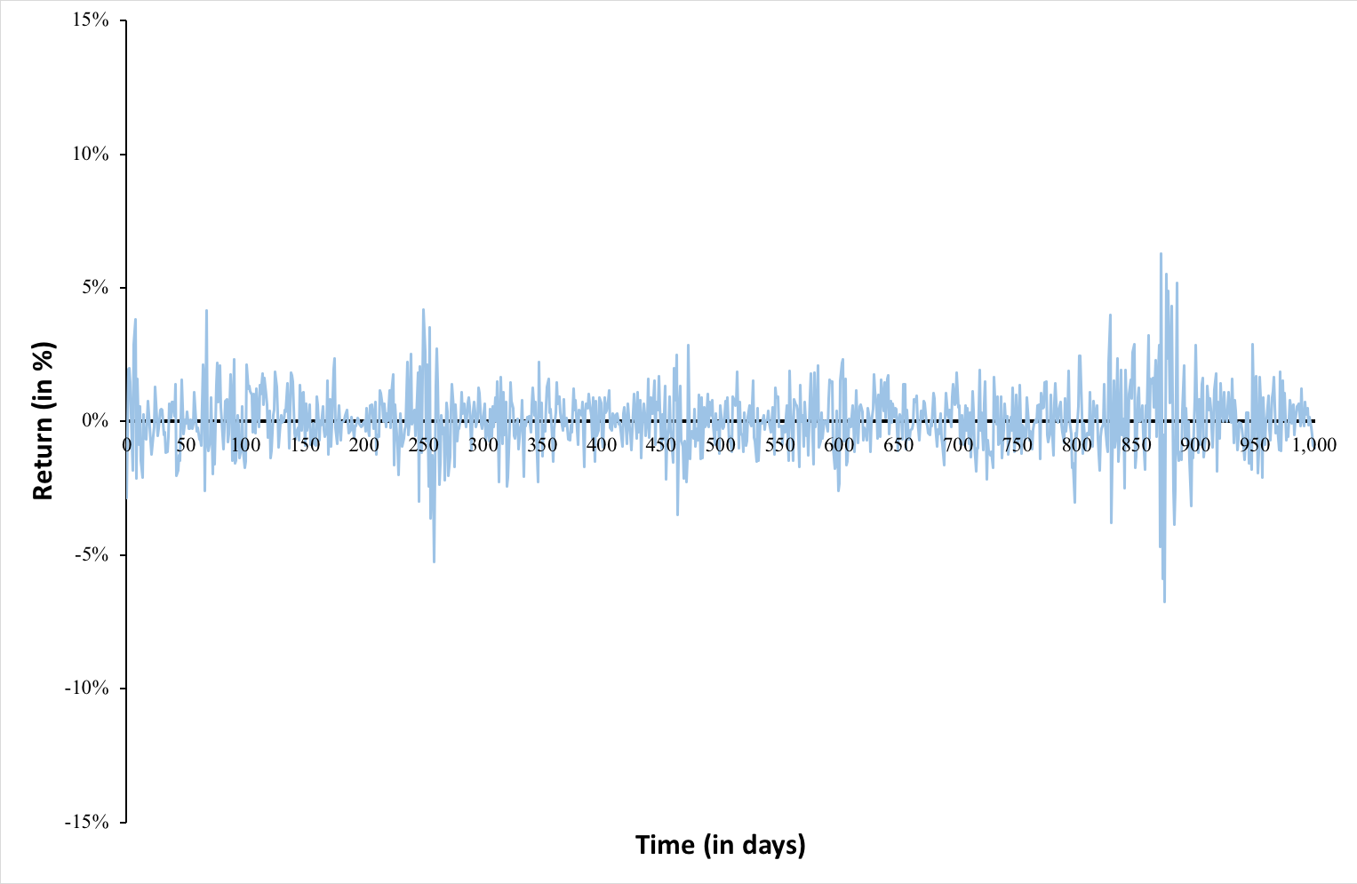
 Computation by the author (data: Bloomberg).
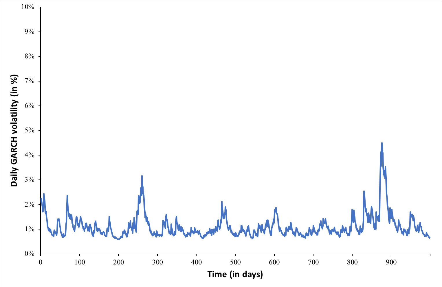