My experience at the startup BSD Investing

My experience at the startup BSD Investing

Rohit SALUNKE

In this article, Rohit SALUNKE (ESSEC Business School, Grande Ecole Program – Master in Management, 2018-2021) shares his experience working in a startup and the evolution of his role and responsibilities…

About BSD Investing

BSD Investing is an independent research firm operating in the asset management industry. It primarily provides research and analysis on active vs passive fund performances for equity and debt funds present across the global financial markets.

The funds are domiciled in Europe (i.e., these are European funds investing in domestic and international markets) and span across 62 universes (i.e., global markets and investment styles).

Logo BDS Investing

The goal of the research is to provide BSD Investing clients with insights into the active vs passive performances and help them optimize the portfolio to get better risk adjusted returns.

The evolution of my missions

I started working at this startup in July 2019 in a small office in Saint-Lazare area in Paris, France. At the beginning, it was just me and two others, the founder, and her colleague. We started from scratch, trying to figure out the best data source to use, figuring out the process flow, the product and much more. After selecting Morningstar as our primary data provider, I began writing codes in Python to fetch the data, create our own portfolios and develop performance key performance indicators (KPIs) for those portfolios. Since we did not have any employee skilled in IT, I was the one who took charge of creating the entire IT architecture from data handling to reporting.

After working for about eight months, we hired our head of IT, and he took over the handling of the IT system and made it much more efficient. That’s when I got the chance to devote my entire focus in developing quantitative models and simulations for the performances of our portfolios.

I started off with researching various technical indicators that gave insights into the market performances and how active funds fared in comparison to passive funds. A major portion of my time was devoted to simulating portfolio performances using various indicator signals. The signals were basically an indication to increase or decrease the active allocation to the portfolio.

Apart from this, I helped a lot with creating marketing materials, conducting market research, interviewing portfolio managers to understand the asset management industry and their needs.

In addition, I work very closely with the IT head to implement our models and key indicators onto the website.

Active and Passive funds

The asset management industry is broadly divided into two management styles: the active style and the passive style. Both styles follow a benchmark that could be an index (e.g., CAC 40), or a combination of indices, or a new portfolio that represent the entire universe of financial instruments in the category that the manager wants to invest in (e.g., Emerging countries large cap ESG funds).

Passive style

The goal of the passive fund manager is to create a portfolio that tracks closely the chosen benchmark. But, since a benchmark consists of a large number of stocks, investing in all of them is not very feasible or cost effective. Therefore, the passive manager creates a portfolio using a smaller number of instruments that aims to replicate the returns from the benchmark.

A good metric to measure the performance of a passive fund is tracking error. It is the divergence between the fund returns and those of the benchmark. A low tracking error means that the fund is tracking the benchmark closely and thus is performing well. Since, a passive fund (also known as ETF or index fund) manager does not aim to outperform the benchmark, but just to simply replicate its returns. Therefore, passive funds charge low fees.

Active style

An active manager on the other hand aims to beat the funds benchmark through stock picking, sector rotation and/or other methods. He or she thus takes a larger risk than a passive fund manager and needs a lot more research, expertise, and management. Therefore, an active fund generally charges more fees than a passive fund. For example, among the France large cap funds, an average passive fund charges around 0.25% of fees, whereas an active manager’s fee may range from 1-2%, in some cases more than 4%.

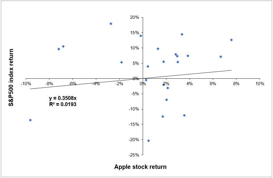
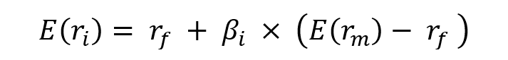
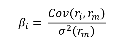
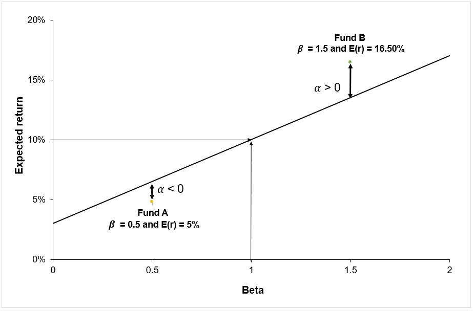
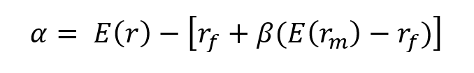
Active managers are alpha seeking. Alpha is the excess return that an active manager generates compared to its benchmark. There are multiple ways to calculate alpha. One such way is using the CAPM model. We predict the expected return of the portfolio using the CAPM model. Subtracting this return from the active managers portfolio gives the alpha. A passive funds alpha is supposed to be zero.

Fund of funds managers create a portfolio of active and/or passive funds to meet their return and risk objectives.

Best style?

In the asset management industry, there is an ongoing debate about which management style is better and are the extra fees charged by the active managers really worth it?

In the US, for example, the active funds have performed very poorly as compared to the ETFs. Whereas, in Europe the performance was mixed and in Japan, the active funds performed better. However, these are the results over the entire period of 10 years. There have been many periods when the active funds outperformed.

Taking the recent example, after the Covid-19 pandemic, the markets went haywire. Since then, in most of the universes active funds have outperformed the passive funds. Therefore, higher returns can be achieved by understanding the markets and allocating the portfolio to the right management style at the right time.

My key learnings

Working in a startup is always challenging and the job comes with heavy responsibilities.

And although working in a startup sounds very interesting, most of the work during the very beginning is quite tedious when it comes to data handling. I spent a few months just understanding the data, checking for errors from the source, figuring out ways to deal with data errors and so on.

Once, I started working on the quantitative models and the simulations, I felt that my work has just begun. During this time, I learnt a big lesson regarding building quantitative models. I build very sophisticated models including machine learning models such as neural networks, gradient boosted trees and so on. However, despite the good results, I had to use simpler logistic models because selling overly sophisticated models would become very difficult.

People in the asset management industry need to know what the real meaning of the data is. And giving recommendations using a black box model does not make it very easy to understand the functioning of the model.

Working on the various indicators, trying to understand their correlations with active and passive fund performances gave me good insights about them. For instance, one good variable that works the best for me is dispersion. This is the standard deviation of returns among funds or stocks. During periods of high dispersion, I observed that active funds generally outperformed the passive funds. I saw a similar result during periods of high volatility. An explanation to this is that a high dispersion could signify a period of high inefficiency in the market, which the active managers could take advantage of. When markets are highly efficient, it makes sense to invest in ETFs, and reduce your costs. Whereas, during periods of high inefficiency, a good active manager could be worth the higher fees that he/she charges. As described above, since March 2019, the active managers have generally outperformed the passive funds across many universes. And this period is also marked with high dispersion and volatility.

In addition, we found that bear periods were more conducive to active outperformance, while bull periods were not. This can be understood since the volatility and dispersion is generally high during bear periods. However, periods after March 2019 were an anomaly to this, since although the markets are in a bull run, there is high dispersion and volatility, and the active funds are outperforming the ETFs.

Knowledge and skills required

For this job I had to have strong data skills, coding skills as well as sound knowledge about finance.
In addition, since I had little to no guidance in my role, I had to come up with my own tasks, define the product and its objects and then learn the essential skills to build it.

Therefore, there was a lot of market research, visits to stackoverflow, reading research papers, cold mailing portfolio managers and so on. Thus, project management and communication skills are essential.

Hard Skills

  • Python
  • SQL
  • HTML
  • MorningstarDirect
  • Capital Markets
  • Portfolio Management, Optimization …
  • Risk Management
  • Market Research

Soft Skills

  • Communication
  • Project Management
  • Leadership
  • Entrepreneurial Thinking
  • Ability to handle pressure
  • Dedication to your project and display of ownership

Related posts on the SimTrade blog

   ▶ All posts about Professional experiences

   ▶ Youssef LOURAOUI Passive Investing

   ▶ Youssef LOURAOUI Active Investing

Useful resources

BSD Investing

Morningstar

About the author

The article was written in December 2021 by Rohit SALUNKE (ESSEC Business School, Grande Ecole Program – Master in Management, 2018-2021).

Beta

Youssef_Louraoui

In this article, Youssef LOURAOUI (Bayes Business School, MSc. Energy, Trade & Finance, 2021-2022) explains the concept of beta, one of the most fundamental concepts in the financial industry, which is heavily used in asset management to assess the risk of assets and portfolios.

This article is structured as follows: we introduce the concept of beta in asset management. Next, we present the mathematical foundations of the concept. We finish with an interpretation of beta values for risk analysis.

Introduction

The (market) beta represents the sensitivity of an individual asset or a portfolio to the fluctuations of the market. This risk measure helps investors to predict the movements of their assets according to the movements of the market overall. It measures the asset risk in comparison with the systematic risk inherent to the market.

In practice, the beta for a portfolio (fund) in respect to the market M represented by a predefined index (the S&P 500 index for example) indicates the fund’s sensitivity to the index. Essentially, the fund’s beta to the index attempts to capture the amount of money made (or lost) when the index increases (or decreases) by a specified amount.

Graphically, the beta represents the slope of the straight line through a regression of data points between the asset return in comparison to the market return for different time periods. It is a traditional risk measure used in the asset management industry. To give a more insightful explanation, a regression analysis has been performed using data for the Apple stock (APPL) and the S&P500 index to see how the stock behaves in relation to the market fluctuations (monthly data for the period July 2018 – June 2020). Figure 1 depicts the regression between Apple stock and the S&P500 index (excess) returns. The estimated beta is between zero and one (beta = 0.3508), which indicates that the stock price fluctuates less than the market index.

Figure 1. Linear regression of the Apple stock return on the S&P500 index return.
Beta analysis for Apple stock return
Source: Computation by the author (data source: Thomson Reuters).

Mathematical derivation of Beta

Use of beta

William Sharpe, John Lintner, and Jan Mossin separately developed key capital markets theory as a result of Markowitz’s previous works: the Capital Asset Pricing Model (CAPM). The CAPM was a huge evolutionary step forward in capital market equilibrium theory since it enabled investors to appropriately value assets in terms of systematic risk, defined as the market risk which cannot be neutralized by the effect of diversification.

The CAPM expresses the expected return of an asset a function of the risk-free rate, the beta of the asset, and the expected return of the market. The main result of the CAPM is a simple mathematical formula that links the expected return of an asset to these different components. For an asset i, it is given by:

CAPM risk beta relation

Where:

  • E(ri) represents the expected return of asset i
  • rf the risk-free rate
  • βi the measure of the risk of asset i
  • E(rm) the expected return of the market
  • E(rm)- rf the market risk premium.

The risk premium for asset i is equal to βi(E(rm)- rf), that is the beta of asset i, βi, multiplied by the risk premium for the market, E(rm)- rf.

In this model, the beta (β) parameter is a key parameter and is defined as:

CAPM beta formula

Where:

  • Cov(ri, rm) represents the covariance of the return of asset i with the return of the market
  • σ2(rm) the variance of the return of the market.

Excel file to compute the beta

You can download below an Excel file with data for Apple stock returns and the S&P500 index returns (used as a representation of the market). This Excel file computes the beta of apple with the S&P500 index.

Download the Excel file to estimate the beta of Apple stock

Interpretation of the beta

Beta helps investors to explain how the asset moves compared to the market. More specifically, we can consider the following cases for beta values:

  • β = 1 indicates a fluctuation between the asset and its benchmark, thus the asset tends to move at a similar rate than the market fluctuations. A passive ETF replicating an index will present a beta close to 1 with its associated index.
  • 0 < β < 1 indicates that the asset moves at a slower rate than market fluctuations. Defensive stocks, stocks that deliver consistent returns without regarding the market state like P&G or Coca Cola in the US, tend to have a beta with the market lower than 1.
  • β > 1 indicates a more aggressive effect of amplification between the asset price movements with the market movements. Call options tend to have higher betas than their underlying asset.
  • β = 0 indicates that the asset or portfolio is uncorrelated to the market. Govies, or sovereign debt bonds, tend to have a beta-neutral exposure to the market.
  • β < 0 indicates an inverse effect of market fluctuation impact in the asset volatility. In this sense, the asset would behave inversely in terms of volatility compared to the market movements. Put options and Gold typically tend to have negative betas.

Why should I be interested in this post?

If you are a business school or university student, this post will help you to understand the fundamentals of investment.

Related posts on the SimTrade blog

   ▶ Youssef LOURAOUI Systematic and specific risks

   ▶ Youssef LOURAOUI Portfolio

   ▶ Youssef LOURAOUI Alpha

   ▶ Jayati WALIA Capital Asset Pricing Model (CAPM)

Useful resources

Academic research

Fama, Eugene F. 1965. The Behavior of Stock Market Prices.Journal of Business 37: January 1965, 34-105.

Fama, Eugene F. 1967. Risk, Return, and General Equilibrium in a Stable Paretian Market. Chicago, IL: University of Chicago.Unpublished manuscript.

Fama, Eugene F. 1968. Risk, Return, and Equilibrium: Some Clarifying Comments. Journal of Finance, (23), 29-40.

Lintner, J. 1965a. The Valuation of Risk Assets and the Selection of Risky Investments in Stock Portfolios and Capital Budgets. The Review of Economics and Statistics 47(1): 13-37.

Lintner, J. 1965b. Security Prices, Risk and Maximal Gains from Diversification. The Journal of Finance 20(4): 587-615.

Mangram, M.E., 2013. A simplified perspective of the Markowitz Portfolio Theory. Global Journal of Business Research, 7(1): 59-70.

Markowitz, H., 1952. Portfolio Selection. The Journal of Finance, 7(1): 77-91.

Mossin, J. 1966. Equilibrium in a Capital Asset Market. Econometrica 34(4): 768-783.

Sharpe, W.F. 1963. A Simplified Model for Portfolio Analysis. Management Science 9(2): 277-293.

Sharpe, W.F. 1964. Capital Asset Prices: A Theory of Market Equilibrium under Conditions of Risk. The Journal of Finance 19(3): 425-442.

Business analysis

JP Morgan Asset Management, 2021. Glossary of investment terms: Beta

Man Institute, 2021. How to calculate the Beta of a portfolio to a factor

Nasdaq, 2021. Beta

About the author

The article was written in November 2021 by Youssef LOURAOUI (Bayes Business School, MSc. Energy, Trade & Finance, 2021-2022).

Alpha

Youssef_Louraoui

In this article, Youssef LOURAOUI (Bayes Business School, MSc. Energy, Trade & Finance, 2021-2022) elaborates on the concept of alpha, one of the fundamental parameters for portfolio performance measure.

This article is structured as follows: we introduce the concept of alpha in asset management. Next, we present some interesting academic findings on the alpha. We finish by presenting the mathematical foundations of the concept.

Introduction

The alpha (also called Jensen’s alpha) is defined as the additional return delivered by the fund manager on the overall performance of the portfolio compared to the market performance (Jensen, 1968). A key issue in finance (and particularly in portfolio management) has been evaluating the performance of portfolio managers. The term ‘performance’ encompasses at least two independent dimensions (Sharpe, 1967): 1) The portfolio manager’s ability to boost portfolio returns by successful forecasting of future security prices; and 2) The portfolio manager’s ability to minimize (via “efficient” diversification) the amount of “insurable risk” borne by portfolio holders.

The primary hurdle to evaluating a portfolio’s performance in these two categories has been a lack of a solid grasp of the nature and assessment of “risk”. Risk aversion appears to predominate in the capital markets, and as long as investors accurately perceive the “riskiness” of various assets, this indicates that “risky” assets must on average give higher returns than less “risky” assets. Thus, when evaluating portfolios’ performance, the implications of varying degrees of risk on their returns must be considered (Sharpe, 1967).

One way of representing the performance is by linking the performance of a portfolio to the security market line (SML). Figure 1 depicts the relation between the portfolio performance in relation to the security market line. As illustrated in Figure 1 below, Fund A has a negative alpha as it is located under the SML, implying a negative performance of the fund manager compared to the market. Fund B has a positive alpha as it is located above the SML, implying a positive performance of the fund manager compared to the market.

Figure 1. Alpha and the Security Market Line

Estimation of alpha

Source: Computation by the author.

You can download below an Excel file with data to compute Jensen’s alpha for fund performance analysis.

Download the Excel file to compute the Jensen's alpha

Academic Literature

Jensen develops a risk-adjusted measure of portfolio performance that quantifies the contribution of a manager’s forecasting ability to the fund’s returns. In the first empirical study to assess the outperformance of fund managers, Jensen aimed at quantifying the predictive ability of 115 mutual fund managers from 1945 to 1964. He looked at their ability to produce returns above the expected return given the risk level of each portfolio. Not only does the evidence on mutual fund performance indicate that these 115 funds on average were unable to forecast security prices accurately enough to outperform a buy-and-hold strategy, but there is also very little evidence that any individual fund performed significantly better than what we would expect from mutual random chance. Additionally, it is critical to highlight that these conclusions hold even when fund returns are measured net of management expenses (that is assume their bookkeeping, research, and other expenses except brokerage commissions were obtained free). Thus, on average, the funds did not appear to be profitable enough in their trading activity to cover even their brokerage expenses.

Mathematical derivation of Jensen’s alpha

The portfolio performance metric given below is derived directly from the theoretical results of Sharpe (1964), Lintner (1965a), and Treynor (1965) capital asset pricing models. All three models assume that (1) all investors are risk-averse and single-period expected utility maximizers, (2) all investors have identical decision horizons and homogeneous expectations about investment opportunities, (3) all investors can choose between portfolios solely based on expected returns and variance of returns, (4) all transaction costs and taxes are zero, and (5) all assets are infinitely fungible. With the extra assumption of an equilibrium capital market, each of the three models produces the following equation for the expected one-period return defined by (Jensen, 1968):

Equation for Jensen's alpha

  • E(r): the expected return of the fund
  • rf: the risk-free rate
  • E(rm): the expected return of the market
  • β(E(rm) – rf): the systematic risk of the portfolio
  • α: the alpha of the portfolio (Jensen’s alpha)

Why should I be interested in this post?

If you are a business school or university student, this post will help you to understand the fundamentals of investment.

Related posts on the SimTrade blog

   ▶ Youssef LOURAOUI Portfolio

   ▶ Youssef LOURAOUI Systematic risk and specific risk

   ▶ Youssef LOURAOUI Beta

   ▶ Youssef LOURAOUI Markowitz Modern Portfolio Theory

   ▶ Jayati WALIA. Capital Asset Pricing Model (CAPM)

Useful resources

Academic research

Fama, Eugene F. 1965. The Behavior of Stock Market Prices.Journal of Business 37, 34-105.

Fama, Eugene F. 1967. Risk, Return, and General Equilibrium in a Stable Paretian Market. Chicago, IL: University of Chicago.Unpublished manuscript.

Fama, Eugene F. 1968. Risk, Return, and Equilibrium: Some Clarifying Comments. Journal of Finance, 23, 29-40.

Lintner, John. 1965a. Security Prices, Risk, and Maximal Gains from Diversification. Journal of Finance, 20, 587-616.

Lintner, John. 1965b. The Valuation of Risk Assets and the Selection of Risky Investments in Stock Portfolios and Capital Budgets.Review of Economics and Statistics 47, 13-37.

Markowitz, H., 1952. Portfolio Selection. The Journal of Finance, 7, 77-91.

Sharpe, William F. 1963. A Simplified Model for Portfolio Analysis. Management Science, 19, 425-442.

Sharpe, William F. 1964. Capital Asset Prices: A Theory of Market Equilibrium under Conditions of Risk. Journal of Finance, 19, 425-442.

Sharpe, William F. 1966. Mutual Fund Performance. Journal of Business39, Part 2: 119-138.

Treynor, Jack L. 1965. How to Rate Management of Investment Funds.Harvard Business Review 18, 63-75.

Business analysis

JP Morgan Asset Management, 2021.Glossary of investment terms: Alpha

About the author

The article was written in November 2021 by Youssef LOURAOUI (Bayes Business School,, MSc. Energy, Trade & Finance, 2021-2022).

Active Investing

Youssef_Louraoui

In this article, Youssef LOURAOUI (Bayes Business School, MSc. Energy, Trade & Finance, 2021-2022) elaborates on the concept of active investing, which is a core investment strategy that relies heavily on market timing and stock picking as the two main drivers of financial performance.

This article is structured as follows: we introduce the concept of active investing in asset management. Next, we present an overview of the academic literature regarding active investing. We finish by presenting some basic principles on active investing.

Introduction

Active investing is an approach for going beyond matching a benchmark’s performance and instead aiming to outperform it. Alpha may be calculated using the CAPM framework, by comparing the fund manager’s expected return with the expected market return (Jensen, 1968). The search for alpha is done through two very different types of investment approaches: stock picking and market timing.

Stock picking

Stock picking is a method used by active managers to select assets based on a variety of variables such as their intrinsic value, the growth rate of dividends, and so on. Active managers use the fundamental analysis approach, which is based on the dissection of economic and financial data that may impact the asset price in the market.

Market timing

Market timing is a trading approach that involves entering and exiting the market at the right time. In other words, when rising outlooks are expected, investors will enter the market, and when downward outlooks are expected, investors will exit. For instance, technical analysis, which examines price and volume of transactions over time to forecast short-term future evolution, and fundamental analysis, which examines the macroeconomic and microeconomic data to forecast future asset prices, are the two techniques on which active managers base their decisions.

Review of academic literature on active investing

As fund managers tried strategies to beat the market, financial literature delved deeper into the mechanism to achieve this purpose. Jensen’s groundbreaking work in the early ’70s gave rise to the concept of alpha in the tracking of a fund’s performance to distinguish between the fund’s manager’s ability to generate abnormal returns and the part of the returns due to luck (Jensen, 1968).

Jensen develops a risk-adjusted measure of portfolio performance that quantifies the contribution of a manager’s forecasting ability to the fund’s returns. He used the measure to quantify the predictive ability of 115 mutual fund managers from 1945 to 1964—that is, their ability to produce returns above those expected given the risk level of each portfolio.

Not only does the evidence on mutual fund performance indicate that these 115 funds on average were unable to forecast security prices accurately enough to outperform a buy-and-hold strategy, but there is also very little evidence that any individual fund performed significantly better than what we would expect from mutual random chance. Additionally, it is critical to highlight that these conclusions hold even when fund returns are measured net of management expenses (that is assume their bookkeeping, research, and other expenses except brokerage commissions were obtained free). Thus, on average, the funds did not appear to be profitable enough in their trading activity to cover even their brokerage expenses.

Core principles of active investing

First principle: market efficiency varies between asset classes.

Investment information is not always readily available in all markets. For less efficient asset classes, an “active” management strategy offers a larger possibility to outperform the market, whereas a “passive” investment strategy may be more appropriate for highly efficient asset classes. In other words, there are compelling advantages for incorporating both active and passive techniques into an overall portfolio.

For example, Wall Street analysts cover a huge portion of US large size shares, making it harder to locate cheap companies. For this highly efficient asset class, a passive investment strategy may be more cost-effective in some cases. On the other side, emerging market equities are sometimes under-researched and difficult to appraise, providing an active manager with additional opportunities to identify mispriced companies. The critical point here is to notice the distinctions and then make the appropriate decisions.

Second principle: market efficiency varies across asset classes.

Within practically every asset class, active and passive management strategies can alternate as winners periodically. Even the most efficient asset classes can occasionally benefit from active management over passive. The reason is substantially distinct from the one stated in Principle One. Principle Two is related to the “Grossman-Stiglitz Paradox”: If markets are fully efficient, there is no reason to investigate them; yet markets can only be perfectly efficient for as long as they are regularly investigated. When investors run out of patience researching stocks in a highly efficient market, passive investment becomes appealing, reopening the door to opportunities for active research. This can result in an annual cycle of active/passive trends.

In some investing environments, active strategies have tended to benefit investors more, while passive strategies have tended to outperform in others. For instance, active managers may outperform more frequently than passive managers when the market is turbulent, or the economy is deteriorating. On the other way, when certain securities within the market move in lockstep or when stock valuations are more consistent, passive strategies may be preferable. Investors may gain from combining passive and active strategies in a way that exploits these insights, depending on the opportunity in various areas of the capital markets. Market conditions, on the other hand, vary constantly, and it frequently takes an intelligent eye to determine when and how much to skew toward passive rather than active investments (Morgan Stanley, 2021).

It’s worth noting that attaining consistently successful active management has historically been more challenging in some asset classes and segments of the market, such as large US company stocks. As a result, it may make sense to be more passive in certain areas and more active in asset classes and segments of the market where active investing has historically been more rewarding, such as overseas stocks in emerging markets and smaller U.S. corporations (Morgan Stanley, 2021).

Why should I be interested in this post?

If you are a business school or university undergraduate or graduate student, this content will help you in broadening your knowledge of finance.

Related posts on the SimTrade blog

   ▶ Youssef LOURAOUI Portfolio

   ▶ Youssef LOURAOUI Systematic and specific risk

   ▶ Youssef LOURAOUI Alpha

   ▶ Youssef LOURAOUI Factor Investing

   ▶ Youssef LOURAOUI Origin of factor investing

   ▶ Youssef LOURAOUI Markowitz Modern Portfolio Theory

   ▶ Jawati WALIA Capital Asset Pricing Model (CAPM)

Useful resources

Academic research

Grossman, S., Stiglitz, J., 1980. On the impossibility of Informationally efficient markets. The American Economic Review, 70(3), 393-408.

Lintner, J. 1965a. The Valuation of Risk Assets and the Selection of Risky Investments in Stock Portfolios and Capital Budgets. The Review of Economics and Statistics 47(1): 13-37.

Lintner, J. 1965b. Security Prices, Risk and Maximal Gains from Diversification. The Journal of Finance, 20(4): 587-615.

Mangram, M.E., 2013. A simplified perspective of the Markowitz Portfolio Theory. Global Journal of Business Research, 7(1): 59-70.

Markowitz, H., 1952. Portfolio Selection. The Journal of Finance, 7(1): 77-91.

Mossin, J. 1966. Equilibrium in a Capital Asset Market. Econometrica, 34(4): 768-783.

Sharpe, W.F. 1963. A Simplified Model for Portfolio Analysis. Management Science, 9(2): 277-293.

Sharpe, W.F. 1964. Capital Asset Prices: A Theory of Market Equilibrium under Conditions of Risk. The Journal of Finance, 19(3): 425-442.

Business analysis

Forbes, 2021. Active or Passive investing? Two principles provide the answer

JP Morgan Asset Management, 2021. Investing

Morgan Stanley, 2021. Active vs Passive management

About the author

The article was written in November 2021 by Youssef LOURAOUI (Bayes Business School, MSc. Energy, Trade & Finance, 2021-2022).