

In this article, Anant JAIN (ESSEC Business School, Grande Ecole Program – Master in Management, 2019-2022) talks about Dow Jones Sustainability Index (DJSI).
Introduction
The Dow Jones Sustainability Index (DJSI) was established in 1999 to honor publicly traded companies that excel in the field of sustainability. As of 2021, it includes 323 companies from a variety of industries that stand out for their outstanding environmental, social, and governance (ESG) performance.
The DJSI was created by S&P Dow Jones Indices (one of the world’s leading resources for benchmark and investable indices) and SAM (corporate sustainability assessment issued by S&P Global) to select the most sustainable companies from 61 industries, combining the experience of an established index provider with the expertise of a specialist in Sustainable Investing.
The indices act as a benchmark for investors who incorporate sustainability considerations into their portfolios, as well as a platform for investors who want to encourage companies to improve their corporate sustainability practices.
Sustainability
Generally speaking, sustainability can be defined as the ability to maintain or support a process over time. Applied to the planet, it refers to the prevention of natural resource depletion to maintain ecological balance for future generations. The term sustainable development was first coined and defined in the 1987 Brundtland Report, Our Common Future, published by the World Commission on Environment and Development of the United Nations (UN): “Development that meets the needs of the present without compromising the ability of future generations to meet their own needs.” In the business context, corporate sustainability is a comprehensive approach to managing operations while ensuring long-term environmental, social, and economic balance. It encompasses a company’s strategies and actions aimed at minimizing negative environmental and social impacts within its market. The sustainability practices of a firm or any organization are typically assessed against environmental, social, and governance (ESG) criteria.
Understanding DJSI
Companies that are included in the DJSI gain not only public recognition and a high level of acceptance from their stakeholders (for their best practices in this field), but they also become a benchmark for many other companies that aspire to be included in the index and want to improve their ranking to be among the best in the world. It is also a key tool for investors, who find these companies appealing and trustworthy, and value them for including policies like these in their strategy, which outperforms other organizations in terms of long-term profitability.
Being accepted into the Dow Jones Sustainability Index is a difficult task. Companies need to pass a rigorous assessment questionnaire with approximately 600 indicators that measure various criteria relating to their corporate governance, code of ethics and conduct, risk management, business, and providers in order to be included in this demanding ranking. Other environmental aspects are also investigated, such as the development of products and programs that are more environmentally friendly and promote efficiency, as well as initiatives aimed at defending human rights, encouraging talent retention and financial inclusion, and improving employee health and well-being.
S&P Global, the world’s largest index provider, is in charge of verifying each of the indicators using a questionnaire with 100 questions about the companies’ environmental, social, and governance performance. The businesses are then graded on a scale of one to one hundred points. Analysts at S&P Global also look at how companies break down public information in their communications with analysts and investors. Only those who achieve the highest ranking in their field of activity are invited to join the DJSI.
Example
MAPFRE is included in the Dow Jones Sustainability World Index for the third year in a row (from 2016 to 2019), with a total score of 77 out of 100. In the areas of customer relationship management, principles for sustainable insurance, social and environmental reporting, and financial inclusion, the company has improved its environmental and social rating and received the highest score (100 points).
MAPFRE has set more than 30 objectives for 2021 to address global issues such as climate change and inequality. It does so as part of its commitment to sustainability and in accordance with its Sustainability Plan 2019–2021, a roadmap that lays out a series of projects aimed at helping the company achieve carbon neutrality, become a leader in the circular economy, promote women’s leadership, and improve financial education, among other objectives.
Methodology
Based on the companies’ Total Sustainability Scores from the annual S&P Global Corporate Sustainability Assessment, the DJSI uses a transparent, rules-based component selection process (CSA). For inclusion in the Dow Jones Sustainability Index family, only the top-ranked companies in each industry are chosen. This process does not exclude any industries. The methodology used by S&P Global to build the DJSI index family is illustrated in Figure 1.
Figure 1. S&P Global methodology for the DJSI index family.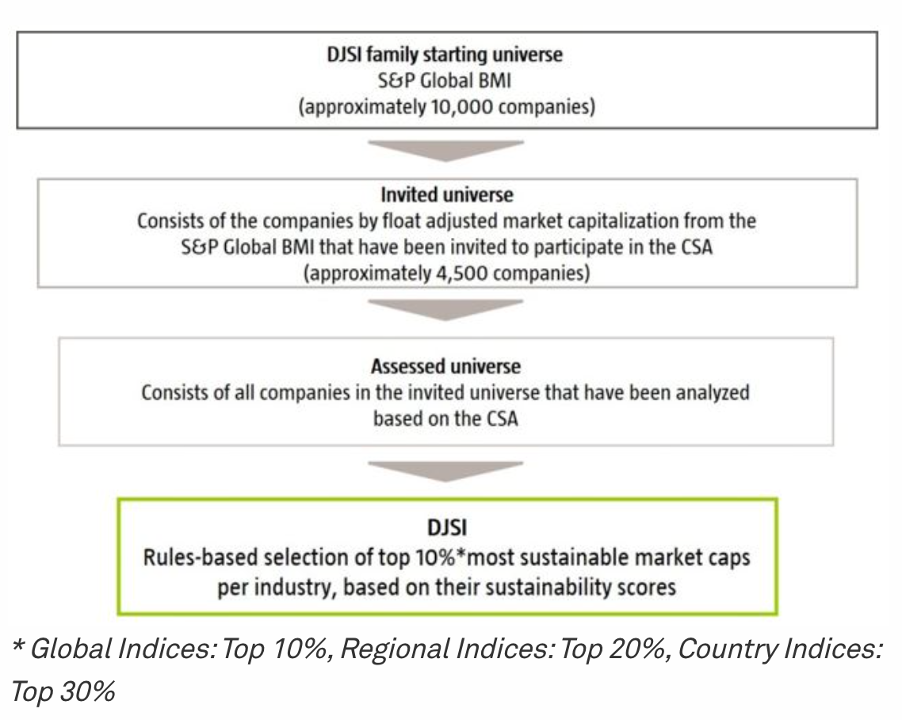
Source: S&P Global.
As mentioned by S&P Global on its website, the DJSI is rebalanced quarterly and is reviewed each year in September based on the S&P Global ESG Scores resulting from the annual SAM CSA.
Index family
As shown in the following list, the Dow Jones Sustainability Index family includes global, regional, and country benchmarks:
- DJSI World
- DJSI North America
- DJSI Europe
- DJSI Asia Pacific
- DJSI Emerging Markets
- DJSI Korea
- DJSI Australia
- DJSI Chile
- DJSI MILA Pacific Alliance
S&P Dow Jones Indices also offers DJSI Indices with exclusion criteria such as Armaments & Firearms, Alcohol, Tobacco, Gambling, and Adult Entertainment for investors who want to limit their exposure to controversial activities.
All DJSI indices are calculated and disseminated in real time, in both price and total return versions.
Related posts on the SimTrade blog
▶ Anant JAIN Environmental, Social & Governance (ESG) Criteria
▶ Anant JAIN MSCI ESG Ratings
Useful resources
Brundtland, G.H. (1987) Our Common Future: Report of the World Commission on Environment and Development.
About the author
The article was written in May 2022 by Anant JAIN (ESSEC Business School, Grande Ecole Program – Master in Management, 2019-2022).
▶ Read all articles by Anant JAIN.


 Computation by the author (data: Bloomberg).