Introduction to Hedge Funds

June 5, 2022 by Youssef LOURAOUI

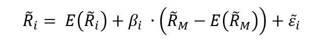
In this article, Youssef LOURAOUI (Bayes Business School, MSc. Energy, Trade & Finance, 2021-2022) elaborates on the concept of Hedge Funds. Hedge funds are a type of asset class that differs from standard fixed-income and equities investments in terms of risk/return profile.

The structure of this article is as follows: First, we will define a hedge fund. Second, we provide a historical perspective on the first known hedge fund. Third, we will discuss hedge fund fees. Fourth, we discuss the conventional long-short strategy and provide an overview of the major hedge fund strategies. And finally, we end by discussing the economic importance of hedge funds.

Introduction

There is no straightforward definition of a hedge fund. Simply said, a hedge fund is an investment vehicle that aims to create performance by employing a variety of complex trading strategies. When the first hedge fund was introduced, the term “hedge” referred to lowering risk by investing in both long and short positions at the same time.

Hedge funds are exempted from the financial regulations that apply to other investment vehicles such as mutual funds. On the one hand, hedge funds have a lot of freedom to implement their investment strategy and face minimal disclosure rules. Hedge funds have the freedom to utilize leverage using derivatives products. On the other hand, hedge funds are restricted in the way they raise money from investors. Hedge fund investors must be “accredited investors,” which means they must have a particular amount of financial wealth and/or financial education to invest. Hedge funds have also been subject to a non-solicitation restriction, which means they are not allowed to advertise or aggressively seek individuals for investment.

According to the Security Exchange Commission (SEC, ), the governmental branch for regulated financial markets in the US, a hedge fund can be defined as follows:

“Hedge fund’ is a general, non-legal term used to describe private, unregistered investment pools that traditionally have been limited to sophisticated, wealthy investors. Hedge funds are not mutual funds and, as such, are not subject to the numerous regulations that apply to mutual funds for the protection of investors – including regulations requiring a certain degree of liquidity, regulations requiring that mutual fund shares be redeemable at any time, regulations protecting against conflicts of interest, regulations to assure fairness in the pricing of fund shares, disclosure regulations, regulations limiting the use of leverage, and more.” (SEC)

The first hedge fund: Jones

In 1949, Alfred Winslow Jones is said to have founded the first professional hedge fund and is regarded as the “father of the hedge fund industry”. He set up the fund as a limited partnership, with the hedge fund manager providing significant initial capital and a few significant investors. The fund’s principal strategy was to use a long/short method, the fund being long on undervalued securities and short on overvalued securities. Jones based his investment approach on stock picking (he believed he lacked market timing skills). Hedge funds’ main idea is that they can use leverage to boost returns in both directions.

From 1955 to 1965, Jones is reported to have achieved a 670% return on his hedge fund by taking both long and short positions. Before Jones, short selling had been popular for a long time, but he realized that by balancing long and short positions, he could be relatively immune to overall market changes while benefiting from the relative outperformance of his long positions against his short positions. The performance of Jones’s fund is shown in Figure 1 about the Dow Jones Industrials index used as a benchmark and Fidelity’s highest performing mutual fund. Over the 1960-65 period, the fund managed to multiply its return by a factor of four, which is higher than the best performing mutual fund (Fidelity Trend Fund) and the Dow-Jones industrials.

Figure 1. Alfred Winslow Jones’s hedge fund performance between 1960-65.
img_SimTrade_jones_performance
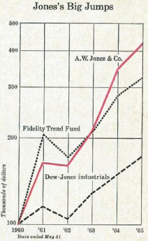
Source: “The Jones Nobody Keeps Up With” (Fortune, 1966).

Development of hedge funds

Interest in hedge funds grew after Fortune magazine published Jones’s results in 1966, and the Securities and Exchange Commission (SEC) listed 140 hedge funds in 1968. As institutional investors began to embrace hedge funds in the 1990s, the hedge fund industry saw a huge spike in interest. Hedge funds with billions of dollars under management were typical in the 2000s, with total hedge fund assets reaching a peak of nearly $2 trillion before the global financial crisis of 2008, dropping during the crisis, and recently reached a new peak.

Hedge funds’ aggregate positions are much larger than their assets under management due to their leverage, and their trading volume is a much larger part of the aggregate trading volume than their relative position sizes due to their high turnover, so hedge fund trading now accounts for a significant portion of all trading. Given a limited demand for liquidity, there is a limited amount of profit to be made and a limited requirement for active investment in an optimally inefficient market, the quantity of capital committed to hedge funds cannot keep expanding.

Hedge funds fees

Among the most frequent fees in the hedge fund industry, we can name the following:

Management fee

Management fee represents the fees that the hedge funds collect to run their operations (salaries, infrastructure, etc.). The management fee is usually about 3%

Performance fee

The performance fee is a compensation when the hedge fund achieves a certain level of performance. This threshold, called the hurdle rate, represents the minimum performance that a hedge fund has to achieve to charge an incentive fee. This motivates the hedge fund manager to perform and to align its interest with its clients’ interests. Beyond the hurdle rate, the outperformance is shared between the hedge fund manager (20%) and the clients (80%).

The high water mark (HWM) provision is a mechanism where the hedge fund will only charge performance fees if it manages to deliver returns above the returns of the previous period. If the hedge fund is down 50%, the performance achieved to recover the losses (100% won’t be subject to performance fees). Only after recovering entirely from the drawdown, the hedge fund can be entitled to earn the performance fee.

A classic hedge fund strategy: the long-short strategy

The long-short strategy is the strategy implemented by the first hedge fund (Alfred Winslow Jones fund). According to Credit Suisse, long-short equity funds engage in both the long and short sides of the equity markets, to diversify or hedge across sectors, regions, and market capitalizations. Managers can switch from value to growth, from small to medium to large capitalization equities, and from net long to net short positions. Managers can also trade stock futures and options, as well as equity-related instruments and debt, and form more concentrated portfolios than classic long-only equity funds.

To illustrate a long-short strategy, we create a hedge fund portfolio based on two stocks from the US equity market. We pick one overvalued stock and one undervalued stock based on their price-to-earnings (P/E) ratio. We chose for this purpose Twitter (overvalued) and Pfizer (undervalued). We download a time series of three-month worth of data for two stocks (Twitter and Pfizer) and the S&P500 index.

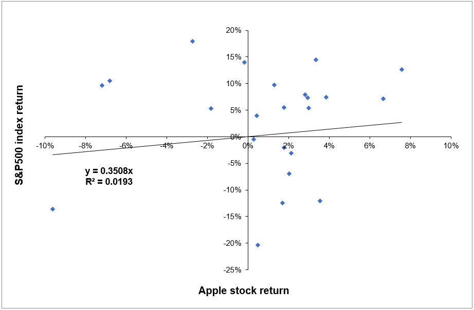
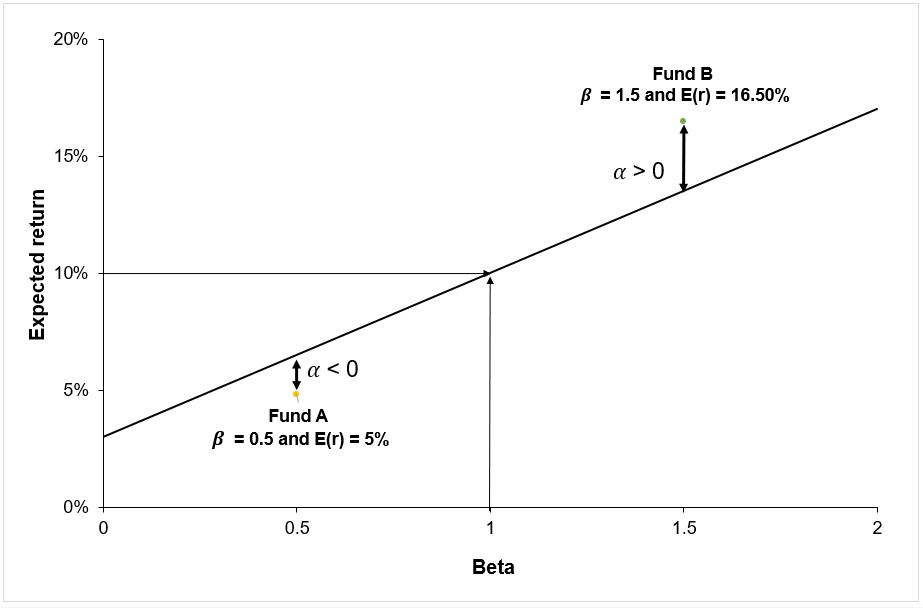
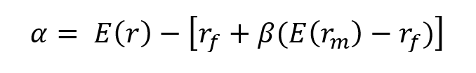
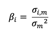
Figure 2 represents the regression of the returns of the simulated hedge fund portfolio on the S&P500 index. We can appreciate a null slope (0.0936) of the regression indicating the low correlation of the hedge fund with the market represented by the S&P500 index. This strategy is market-neutral, meaning that the portfolio is not correlated directly with the market fluctuations. The performance of a zero-beta portfolio would be derived from the alpha, a key metric in the portfolio management industry.

Figure 2. Regression of the hedge fund return on the S&P500 market index.
Hedge fund portfolio regression
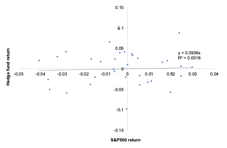
Source: computation by the author (data: Bloomberg).

We compute the return and volatility of each security and the market index as a starting point. We also determine the correlation of the stocks to the market index. For the short position (Twitter), the sign of the correlation inverts of the sign. We compute an equally-weighted portfolio composed of two stocks: a long position on Pfizer and a short position on Twitter. This portfolio delivered a return of 0.27%, which is better than the broader stock index return over the same period (-0.22%).

Figure 3 depicts the return of the hedge fund portfolio relative to the market index return. From the analysis, the long-short strategy managed to outperform the S&P500 market index by 49 basis points. Even if the market is in a bearish setting, the strategy managed to deliver positive returns as the short position helps to be uncorrelated the return of the hedge fund from the market return.

Figure 3. Return of the hedge fund relative to the S&P500 market index.
Long short strategy performance
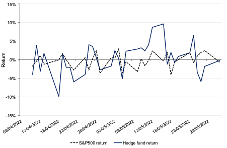
Source: computation by the author (data: Bloomberg).

You can download below the Excel file below which gives the details of the computation of the long-short strategy example.

Hedge fund role in economy

Hedge funds, for example, are frequently criticized in the media. Companies, for example, dislike seeing their shares shorted because it indicates a belief that the company’s share price will fall. Short sellers, including hedge funds, are sometimes blamed for a company’s problems, even though the stock price is usually falling due to the company’s poor financial condition, not because of any other source.

Hedge funds, in general, serve several important functions in the economy. First, they improve market efficiency by gathering information about businesses and incorporating it into prices through their trades. Because the capital market is the tool used to allocate resources in the economy, increased efficiency can improve real economic outcomes. Companies with good growth prospects see their share prices rise when markets are efficient, allowing them to raise capital and fund new projects. Companies that produce goods and services that are no longer required to see their share prices fall and the factories may be repurposed for more productive purposes, possibly leading to a merger. Furthermore, when share prices reflect more information and are more efficient, CEO decisions may improve, and they may be more prudent if active investors are monitoring them. Hedge funds also serve as a source of liquidity for other investors who need to buy or sell (e.g., to smooth out their consumption), hedge or buy insurance, or simply enjoy certain types of securities. Finally, hedge funds offer investors another source to diversify their returns.

Why should I be interested in this post?

As an investor, hedge funds may provide an opportunity to diversify its global portfolios. Including hedge funds in a portfolio can help investors obtain absolute returns that are uncorrelated with typical bond/equity returns.

For practitioners, learning how to incorporate hedge funds into a standard portfolio and understanding the risks associated with hedge fund investing can be beneficial.

Understanding if hedge funds are truly providing “excess returns” and deconstructing the sources of return can be beneficial to academics. Another challenge is determining whether there is any “performance persistence” in hedge fund returns.

Getting a job at a hedge fund might be a profitable career path for students. Understanding the market, the players, the strategies, and the industry’s current trends can help you gain a job as a hedge fund analyst or simply enhance your knowledge of another asset class.

Useful resources

Academic research

Pedersen, L. H., 2015. Efficiently Inefficient: How Smart Money Invests and Market Prices Are Determined. Princeton University Press.

Business Analysis

Wikipedia Alfred Winslow Jones

Fortune (2015) The Jones Nobody Keeps Up With (Fortune, 1966).

SEC Mutual Funds and Exchange-Traded Funds (ETFs) – A Guide for Investors.

SEC Selected Definitions of “Hedge Fund”

Credit Suisse Hedge fund strategy

Credit Suisse Hedge fund performance

Credit Suisse Long-short strategy

Credit Suisse Long-short performance benchmark

About the author

The article was written in June 2022 by Youssef LOURAOUI (Bayes Business School, MSc. Energy, Trade & Finance, 2021-2022).

Specific risk

April 1, 2022 by Youssef LOURAOUI

In this article, Youssef LOURAOUI (Bayes Business School, MSc. Energy, Trade & Finance, 2021-2022) explains the specific risk of financial assets, a key concept in asset pricing models and asset management in practice.

This article is structured as follows: we start with a reminder of portfolio theory and the central concept of risk in financial markets. We then introduce the concept of specific risk of an individual asset and especially its sources. We then detail the mathematical foundation of risk. We finish with an insight of the relationship between diversification and risk reduction with a practical example to test this concept.

Portfolio Theory and Risk

Markowitz (1952) and Sharpe (1964) created a framework for risk analysis based on their seminal contributions to portfolio theory and capital market theory. All rational profit-maximizing investors attempt to accumulate a diversified portfolio of risky assets and borrow or lend to achieve a risk level consistent with their risk preferences given a set of assumptions. They established that the key risk indicator for an individual asset in these circumstances is its correlation with the market portfolio (the beta).

The variance of returns of an individual asset can be decomposed as the sum of systematic risk and specific risk. Systematic risk refers to the proportion of the asset return variance that can be attributed to the variability of the whole market. Specific risk refers to the proportion of the asset return variance that is unconnected to the market and reflects the unique nature of the asset. Specific risk is often regarded as insignificant or irrelevant because it can be eliminated in a well-diversified portfolio.

Sources of specific risk

Specific risk can find its origin in business risk (in the assets side of the balance sheet) and financial risk (in the liabilities side of the balance sheet):

Business risk

Internal or external issues might jeopardize a business. Internal risk is directly proportional to a business’s operational efficiency. An internal risk would include management neglecting to patent a new product, so eroding the company’s competitive advantage.

Financial risk

This pertains to the capital structure of a business. To continue growing and meeting financial obligations, a business must maintain an ideal debt-to-equity ratio.

Mathematical foundations

Following the Capital Asset Pricing Model (CAPM), the return on asset i, denoted by R_i can be decomposed as

img_SimTrade_return_decomposition

Where:

R_i the return of asset i
E(R_i) the risk premium of asset i
β_i the measure of the risk of asset i
R_M the return of the market
E(R_M) the risk premium of the market
R_M – E(R_M) the market factor
ε_i represent the specific part of the return of asset i

The three components of the decomposition are the expected return, the market factor and an idiosyncratic component related to asset only. As the expected return is known over the period, there are only two sources of risk: systematic risk (related to the market factor) and specific risk (related to the idiosyncratic component).

The beta of the asset with the market is computed as:

Beta

Where:

σ_i,m : the covariance of the asset return with the market return
σ_m² : the variance of market return

The total risk of the asset measured by the variance of asset returns can be computed as:

Decomposition of total risk

Where:

β_i² * σ_m² = systematic risk
σ_εi² = specific risk

In this decomposition of the total variance, the first component corresponds to the systematic risk and the second component to the specific risk.

Decomposition of returns

We analyze the decomposition of returns on Apple stocks. Figure 1 gives for every month of 2021 the decomposition of Apple stock returns into three parts: expected return, market factor (systematic return) and an idiosyncratic component (specific return). We used historical price downloaded from the Bloomberg terminal for the period 1999-2022.

Figure 1. Decomposition of Apple stock returns:
expected return, systematic return and specific return.
Decomposition of asset returns Computation by the author (data: Bloomberg).

You can download below the Excel file which illustrates the decomposition of returns on Apple stocks.

Why should I be interested in this post?

Investors will be less influenced by single incidents if they possess a range of firm stocks across several industries, as well as other types of assets in a number of asset classes, such as bonds and stocks.

An investor who only bought telecommunication equities, for example, would be exposed to a high amount of unsystematic risk (also known as idiosyncratic risk). A concentrated portfolio can have an impact on its performance. This investor would spread out telecommunication-specific risks by adding uncorrelated positions to their portfolio, such as firms outside of the telecommunication market.

Useful resources

Academic research

Evans, J.L., Archer, S.H. 1968. Diversification and the Reduction of Dispersion: An Empirical Analysis. The Journal of Finance, 23(5): 761–767.

Markowitz, H. 1952. Portfolio Selection. The Journal of Finance, 7(1): 77-91.

Mossin, J. 1966. Equilibrium in a Capital Asset Market. Econometrica, 34(4): 768-783.

Sharpe, W.F. 1963. A Simplified Model for Portfolio Analysis. Management Science, 9(2): 277-293.

Sharpe, W.F. 1964. Capital Asset Prices: A Theory of Market Equilibrium under Conditions of Risk. The Journal of Finance, 19(3): 425-442.

Tole T.M. 1982. You can’t diversify without diversifying. The Journal of Portfolio Management. Jan 1982, 8 (2) 5-11.

About the author

The article was written in April 2022 by Youssef LOURAOUI (Bayes Business School, MSc. Energy, Trade & Finance, 2021-2022).

Systematic risk

April 1, 2022 by Youssef LOURAOUI

In this article, Youssef LOURAOUI (Bayes Business School, MSc. Energy, Trade & Finance, 2021-2022) presents the systematic risk of financial assets, a key concept in asset pricing models and investment management theories more generally.

This article is structured as follows: we introduce the concept of systematic risk. We then explain the mathematical foundation of this concept. We present an economic understanding of market risk on recent events.

Portfolio Theory and Risk

Markowitz (1952) and Sharpe (1964) developed a framework on risk based on their significant work in portfolio theory and capital market theory. All rational profit-maximizing investors seek to possess a diversified portfolio of risky assets, and they borrow or lend to get to a risk level that is compatible with their risk preferences under a set of assumptions. They demonstrated that the key risk measure for an individual asset is its covariance with the market portfolio under these circumstances (the beta).

The fraction of an individual asset’s total variance attributable to the variability of the total market portfolio is referred to as systematic risk, which is assessed by the asset’s covariance with the market portfolio. Systematic risk can be decomposed into the following categories:

Interest rate risk

We are aware that central banks, such as the Federal Reserve, periodically adjust their policy rates in order to boost or decrease the rate of money in circulation in the economy. This has an effect on the interest rates in the economy. When the central bank reduces interest rates, the money supply expands, allowing companies to borrow more and expand, and when the policy rate is raised, the reverse occurs. Because this is cyclical in nature, it cannot be diversified.

Inflation risk

When inflation surpasses a predetermined level, the purchasing power of a particular quantity of money reduces. As a result of the fall in spending and consumption, overall market returns are reduced, resulting in a decline in investment.

Exchange Rate Risk

As the value of a currency reduces in comparison to other currencies, the value of the currency’s returns reduces as well. In such circumstances, all companies that conduct transactions in that currency lose money, and as a result, investors lose money as well.

Geopolitical Risks

When a country has significant geopolitical issues, the country’s companies are impacted. This can be mitigated by investing in multiple countries; but, if a country prohibits foreign investment and the domestic economy is threatened, the entire market of investable securities suffers losses.

Natural disasters

All companies in countries such as Japan that are prone to earthquakes and volcanic eruptions are at risk of such catastrophic calamities.

Following the Capital Asset Pricing Model (CAPM), the return on asset i, denoted by R_i can be decomposed as

img_SimTrade_return_decomposition

Where:

R_i the return of asset i
E(R_i) the risk premium of asset i
β_i the measure of the risk of asset i
R_M the return of the market
E(R_M) the risk premium of the market
R_M – E(R_M) the market factor
ε_i represent the specific part of the return of asset i

The beta of the asset with the market is computed as:

Beta

Where:

σ_i,m : the covariance of the asset return with the market return
σ_m² : the variance of market return

The total risk of the asset measured by the variance of asset returns can be computed as:

Decomposition of total risk

Where:

β_i² * σ_m² = systematic risk
σ_εi² = specific risk

In this decomposition of the total variance, the first component corresponds to the systematic risk and the second component to the specific risk.

Systematic risk analysis in recent times

The volatility chart depicts the evolution of implied volatility for the S&P 500 and US Treasury bonds – the VIX and MOVE indexes, respectively. Implied volatility is the price of future volatility in the option market. Historically, the two markets have been correlated during times of systemic risk, like as in 2008 (Figure 1).

Figure 1. Volatility trough time (VIX and MOVE index).

Sources: BlackRock Risk and Quantitative Analysis and BlackRock Investment Institute, with data from Bloomberg and Bank of America Merrill Lynch, October 2021 (BlackRock, 2021).

The VIX index has declined following a spike in September amid the equity market sell-off. It has begun to gradually revert to pre-Covid levels. The periodic, albeit brief, surges throughout the year underscore the underlying fear about what lies beyond the economic recovery and the possibility of a wide variety of outcomes. The MOVE index — a gauge of bond market volatility – has remained relatively stable in recent weeks, despite the rise in US Treasury yields to combat the important monetary policy to combat the effect of the pandemic. This could be a reflection of how central banks’ purchases of government bonds are assisting in containing interest rate volatility and so supporting risk assets (BlackRock, 2021).

The regime map depicts the market risk environment in two dimensions by plotting market risk sentiment and the strength of asset correlations (Figure 2).

Figure 2. Regime map for market risk environment.

Source: BlackRock Risk and Quantitative Analysis and BlackRock Investment Institute, October 2021 (BlackRock, 2021).

Positive risk sentiment means that riskier assets, such as equities, are outperforming less risky ones. Negative risk sentiment means that higher-risk assets underperform lower-risk assets.

Due to the risk of fast changes in short-term asset correlations, investors may find it challenging to guarantee their portfolios are correctly positioned for the near future. When asset correlation is higher (as indicated by the right side of the regime map), diversification becomes more difficult and risk increases. When asset prices are less correlated (on the left side of the map), investors have greater diversification choices.

When both series – risk sentiment and asset correlation – are steady on the map, projecting risk and return becomes easier. However, when market conditions are unpredictable, forecasting risk and return becomes substantially more difficult. The map indicates that we are still in a low-correlation environment with a high-risk sentiment, which means that investors are rewarded for taking a risk (BlackRock, 2021). In essence, investors should use diversification to reduce the specific risk of their holding coupled with macroeconomic fundamental analysis to capture the global dynamics of the market and better understand the sources of risk.

Why should I be interested in this post?

Market risks fluctuate throughout time, sometimes gradually, but also in some circumstances dramatically. These adjustments typically have a significant impact on the right positioning of a variety of different types of investment portfolios. Investors must walk a fine line between taking enough risks to achieve their objectives and having the proper instruments in place to manage sharp reversals in risk sentiment.

Useful resources

Academic research

Markowitz, H. 1952. Portfolio Selection. The Journal of Finance, 7(1): 77-91.

Mossin, J. 1966. Equilibrium in a Capital Asset Market. Econometrica, 34(4): 768-783.

Sharpe, W.F. 1963. A Simplified Model for Portfolio Analysis. Management Science, 9(2): 277-293.

Sharpe, W.F. 1964. Capital Asset Prices: A Theory of Market Equilibrium under Conditions of Risk. The Journal of Finance, 19(3): 425-442.

Business analysis

BlackRock, 2021. Market risk monitor

About the author

The article was written in April 2022 by Youssef LOURAOUI (Bayes Business School, MSc. Energy, Trade & Finance, 2021-2022).

Implementing Black-Litterman asset allocation model

March 21, 2022 by Youssef LOURAOUI

In this article, Youssef Louraoui (Bayes Business School, MSc. Energy, Trade & Finance, 2021-2022) presents an implementation of the Black-Litterman model, used to determine the expected return of a portfolio by integrating investor’s views regarding the performance of the underlying assets selected in the investment portfolio.

This article follows the following structure: first, we introduce the Black-Litterman model. We then present the mathematical foundations of this model. We conclude with an explanation of the methodology to build the spreadsheet with the results obtained. You will find in this post an Excel spreadsheet which implement the model.

Introduction

The Black-Litterman asset allocation model, established for the first time in the early 1990’s by Fischer Black and Robert Litterman, is a sophisticated strategy for dealing with unintuitive, highly concentrated, and input-sensitive portfolios. The most likely reason that more portfolio managers do not use the Markowitz model, which maximises return for a given degree of risk, is input sensitivity, a well-documented issue with mean-variance optimization.

The Black-Litterman Model employs a Bayesian technique to integrate an investor’s subjective views of expected returns on one or more assets with the market equilibrium vector (prior distribution) of expected returns to obtain a new, mixed estimate of expected returns. The new vector of returns (the posterior distribution) is a weighted complex average of the investor’s views and market equilibrium.

Mathematical foundation

The idea of the Black Litterman estimates is not to find the optimum portfolio weights as in the Markowitz optimization framework, but instead to find the expected return that would be used as an input to compute the optimum portfolio weights. This approach is referred as reversion portfolio optimization technique. The idea behind is that optimum weights are already observed in the market and captured in the market portfolio. We can approach the reasoning by maximizing the following utility function adjusted to the risk:

img_SimTrade_mathematical_foundation_Black_Litterman_6

w^T = transposed of portfolio weights
Π = Implied equilibrium excess return vector
A = price of risk or risk aversion factor
Σ = variance-covariance matrix

We take the partial derivative of U in terms of weights (w) and we derive the following expression:

img_SimTrade_mathematical_foundation_Black_Litterman_5

By setting the partial derivative equal to zero, we can maximize the utility function in term of weights. The proposed approach in the Black Litterman approach is that instead of seeking the optimal weights, which are incorporated in the market portfolio and thus computable via the market capitalization of the equities in the portfolio, we’ll isolate the Π (implied equilibrium excess return) to obtain the optimal expected returns for the portfolio:

We can deconstruct the Black-Litterman model as

img_SimTrade_mathematical_foundation_Black_Litterman_3

τ= scalar
P = Linking matrix
∑ = Variance-covariance matrix
Π= implied equilibrium excess return
A = Price of risk
w = weight vector
Ω = uncertainty of views

The first term of the formula is introduced in order to respect the constraint that the portfolio weights should be equal to one:

The second term of the formula is to compute a weighted average of the implied equilibrium excess return adjusted to the uncertainty of the returns by the view vector weighted with the uncertainty of views:

The final output E(R) is a vector of return n x 1 that represent the equilibrium returns of the market adjusted to investors views.

Implementation of the Black-Litterman asset allocation model in practice

To model a Black-Litterman portfolio allocation, we obtained a large time series to obtain useful results by downloading the equivalent of 23 years of market data from a data provider (in this example, Bloomberg). We generate the variance-covariance matrix after obtaining all necessary statistical data, which includes the expected return and volatility indicated by the standard deviation of the returns for each stock during the provided period.

The data is derived from the Bloomberg terminal. The first step is to calculate the logarithmic returns and excess returns on the selected assets (returns minus the risk-free rate). After calculating the logarithmic returns on each asset, we can estimate the capital asset pricing model’s returns (CAPM) expected returns. This information will be used to calculate the Black-Litterman expected returns on a comparative basis.

1. The first input for the model is the price of risk A, which represents the risk aversion of investor and is obtained by subtracting the expected return of the market the risk-free rate and divided by the variance of the market:

img_SimTrade_Black_Litterman_formulas_for_spreadsheet_1

E(r_m)= expected market returns
r_f = risk-free rate
σ²_m = variance of market

2. We extract the respective market capitalization of each security to obtain their market weights in the portfolio. Given that our investable universe is made of five stocks, we can retrieve their respective market capitalization and compute the weights of each stock in relation to the sum of total market-capitalization in the portfolio.

img_SimTrade_Black_Litterman_formulas_for_spreadsheet_2

Table 1 depicts the optimal weights obtained from their respective market capitalisation, coupled with the respective expected return and volatility.

Table 1. Asset characteristics of Apple, Amazon, Microsoft, Goldman Sachs, and Pfizer.

img_SimTrade_Black_Litterman_spreadsheet_2

Source: computation by the author.

3. We compute the variance-covariance matrix of logarithmic returns using the data analysis tool pack available in Excel (Table 2).

Table 2. Variance-covariance matrix of asset returns

img_SimTrade_Black_Litterman_spreadsheet_5

Source: computation by the author.

4. We compute the implied equilibrium excess return (Π) as the matrix calculation of the price of risk (A) times the matrix multiplication of the weights computed in step 4 times the variance-covariance matrix computed in step 3.

img_SimTrade_Black_Litterman_formulas_for_spreadsheet_3

Π= implied equilibrium excess return
A = Price of risk
w = weight vector

5. The views are incorporated into the model. To achieve this, we provide three views to include into the model. If there are no views, the values will correspond to the market portfolio. The investment manager’s views for the expected return on certain of the portfolio’s assets regularly diverge from the Implied Equilibrium Return Vector (), which serves as the market-neutral starting point for the Black-Litterman model that quantifies the uncertainty associated with each view. The Black-Litterman Model can be used to depict such views in absolute or relative terms. As an illustration, let us suppose that the real and simulated portfolio will have the same views:

View 1: Apple will outperform Microsoft by .05 percent
View 2: Amazon will outperform Microsoft by .1 percent
View 3: Apple will outperform Amazon by .05 percent

To incorporate the vector Q of views, we create a link matrix P where the rows sum to zero. Figure 3 depicts the workings done in the spreadsheet.

Table 3. Views vector and Link Matrix (P)

img_SimTrade_Black_Litterman_spreadsheet_1

Source: computation by the author.

6. We compute omega to determine the degree of uncertainty associated with the views. While Black-Litterman paper used a value of tau equal to 0.25, an important number of academics went for calculating the tau equal to one. For the sake of simplifying the model, consider tau to be equal to one. This input is obtained by multiplying the Linking matrix by the variance-covariance matrix and transposing the Linking matrix (P).

img_SimTrade_Black_Litterman_formulas_for_spreadsheet_4

τ= scalar
P = Linking matrix
∑ = Variance-covariance matrix

7. We integrate all the values computed previously in the Black-Litterman model. Table 4 depicts the results obtained via the Black-Litterman allocation model.

Table 4. Results of the Black-Litterman allocation

img_SimTrade_Black_Litterman_spreadsheet_4

Source: computation by the author.

We can see that the results converge slightly to those from CAPM. Additionally, we can see that the views are reflected in the Black-Litterman expected returns. As a result, we can determine whether or not each view is satisfied. Indeed, Apple outperforms Amazon and Microsoft, while Amazon outperforms Microsoft.

You can download an Excel file to help you construct a portfolio via the Black-Litterman allocation model.

Why should I be interested in this post?

Modern Portfolio Theory is at the heart of modern finance, shaping the modern investing landscape. MPT has become the cornerstone of current financial theory and practice. MPT’s thesis is that winning the market is difficult and requires diversification and taking higher-than-average risks.

MPT has been around for nearly sixty years and shows no signs of slowing down. His theoretical contributions paved the way for more portfolio theory study. But Markowitz’s portfolio theory is sensitive to and depends on further ‘probabilistic’ expansion. This paper expanded on Markowitz’s previous work by incorporating investor views into the asset allocation process.

Useful resources

Academic research

Black, F. and Litterman, R. 1990. Asset Allocation: Combining Investors Views with Market Equilibrium. Goldman Sachs Fixed Income Research working paper

Black, F. and Litterman, R. 1991. Global Asset Allocation with Equities, Bonds, and Currencies. Goldman Sachs Fixed Income Research working paper

Black, F. and Litterman, R. 1992. Global Portfolio Optimization.Financial Analysts Journal, 28-43.

Idzorek, T.M. 2002. A step-by-step guide to Black-Litterman model. Incorporating user-specified confidence levels. Working Paper, 2-11.

Markowitz, H., 1952. Portfolio Selection. The Journal of Finance, 7(1): 77-91.

About the author

The article was written in Mars 2022 by Youssef LOURAOUI (Bayes Business School, MSc. Energy, Trade & Finance, 2021-2022).

Implementing Markowitz asset allocation model

March 20, 2022 by Youssef LOURAOUI

In this article, Youssef LOURAOUI (Bayes Business School, MSc. Energy, Trade & Finance, 2021-2022) explains how to implement the Markowitz asset allocation model. This model is used to determine optimal asset portfolios based on the risk-return trade-off.

This article follows the following structure: first, we introduce the Markowitz model. We then present the mathematical foundations of this model. We conclude with an explanation of the methodology to build the spreadsheet with the results obtained. You will find in this post an Excel spreadsheet which implements the Markowitz asset allocation model.

Introduction

Markowitz’s work is widely regarded as a pioneer work in financial economics and corporate finance due to its theoretical foundations and applicability in the financial sector. Harry Markowitz received the Nobel Prize in 1990 for his contributions to these disciplines, which he outlined in his 1952 article “Portfolio Selection” published in The Journal of Finance. His major work established the foundation for what is now commonly referred to as “Modern Portfolio Theory” (MPT).

To find the portfolio’s minimal variance, the Markowitz model uses a constrained optimization strategy. The goal of the Markowitz model is to take into account the expected return and volatility of the assets in the investable universe to provide an optimal weight vector that indicates the best allocation for a given level of expected return or the best allocation for a given level of volatility. The expected return, volatility (standard deviation of expected return), and the variance-covariance matrix to reflect the co-movement of each asset in the overall portfolio design are the major inputs for this portfolio allocation model for an n-asset portfolio. We’ll go over how to use this complex method to find the best portfolio weights in the next sections.

Mathematical foundations

The investment universe is composed of N assets characterized by their expected returns μ and variance-covariance matrix V. For a given level of expected return μ_P, the Markowitz model gives the composition of the optimal portfolio. The vector of weights of the optimal portfolio is given by the following formula:

With the following notations:

w_P = vector of asset weights of the portfolio
μ_P = desired level of expected return
e = identity vector
μ = vector of expected returns
V = variance-covariance matrix of returns
V^-1 = inverse of the variance-covariance matrix
t = transpose operation for vectors and matrices

A, B and C are intermediate parameters computed below:

img_SimTrade_implementing_Markowitz_2

The variance of the optimal portfolio is computed as follows

img_SimTrade_implementing_Markowitz_3

To calculate the standard deviation of the optimal portfolio, we take the square root of the variance.

Implementation of the Markowitz asset allocation model in practice

We generated a large time series to obtain useful results by downloading the equivalent of 23 years of market data from a data provider (in this example, Bloomberg). We generate the variance-covariance matrix after obtaining all necessary statistical data, which includes the expected return and volatility indicated by the standard deviation of the returns for each stock during the provided period. Table 1 depicts the expected return and volatility for each stock retained in this analysis.

Table 1. Asset characteristics of Apple, Amazon, Microsoft, Goldman Sachs, and Pfizer.
img_SimTrade_implementing_Markowitz_spreadsheet_1
Source: computation by the author.

We use the data analysis tool pack supplied in Excel to run a variance-covariance matrix for ease of computation (Table 2).

Table 2. Variance-covariance matrix of asset returns.
img_SimTrade_implementing_Markowitz_spreadsheet_4
Source: computation by the author.

We can start the optimization task by setting a desirable expected return after computing the expected return, volatility, and the variance-covariance matrix of expected return. With the data that is fed into the appropriate cells, the model will complete the optimization task. For a 10% desired expected return, we get the following results (Table 3).

Table 3. Asset weights for an optimal portfolio.
img_SimTrade_implementing_Markowitz_spreadsheet_2
Source: computation by the author.

To demonstrate the effect of diversification in the reduction of volatility, we can form a Markowitz efficient frontier by tilting the desired anticipated return with their relative volatility in a graph. The Markowitz efficient frontier is depicted in Figure 1 for various levels of expected return (Figure 1).

Figure 1. Markowitz efficient portfolio frontier.
img_SimTrade_implementing_Markowitz_spreadsheet_3
Source: computation by the author.

You can download the Excel file below to use the Markowitz portfolio allocation model.

Why should I be interested in this post?

Modern Portfolio Theory (MPT) is at the heart of modern finance, shaping the modern investing landscape. MPT has become the cornerstone of current financial theory and practice. MPT has been around for nearly sixty years and shows no signs of slowing down. His theoretical contributions paved the way for more portfolio theories. This post helps you to grasp the theoretical model and its implementation.

Useful resources

Academic research

Petters, A. O., and Dong, X. 2016. An Introduction to Mathematical Finance and Applications. Springer Undergraduate Texts in Mathematics and Technology.

Markowitz, H., 1952. Portfolio Selection. The Journal of Finance, 7(1): 77-91.

About the author

The article was written in Mars 2022 by Youssef LOURAOUI (Bayes Business School, MSc. Energy, Trade & Finance, 2021-2022).

Systematic risk and specific risk

November 30, 2021 by Youssef LOURAOUI

In this article, Youssef LOURAOUI (Bayes Business School, MSc. Energy, Trade & Finance, 2021-2022) presents the systematic risk and specific risk of financial assets, two fundamental concepts in asset pricing models and investment management theories more generally.

This article is structured as follows: we introduce the concept of systematic and specific risk. We then explain the mathematical foundation of this concept. We finish with an insight that sheds light on the relationship between diversification and risk reduction.

Portfolio Theory and Risk

The fraction of an individual asset’s total variance attributable to the variability of the total market portfolio is referred to as systematic risk, which is assessed by the asset’s covariance with the market portfolio. In the article systematic risk, we develop the economic sources of systematic risk: interest rate risk, inflation risk, exchange rate risk, geopolitical risk, and natural risk.

Additionally, due to the asset’s unique characteristics, an individual asset exhibits variance that is unrelated to the market portfolio (the asset’s non-market variance). Specific risk is the term for non-market variance, and it is often seen as minor because it can be eliminated in a large diversified portfolio. In the article specific risk, we develop the economic sources of specific risk: business risk and financial risk.

Mathematical foundations

Following the Capital Asset Pricing Model (CAPM), the return on asset i, denoted by R_i can be decomposed as

img_SimTrade_return_decomposition

Where:

R_i the return of asset i
E(R_i) the expected return of asset i
β_i the measure of the risk of asset i
R_M the return of the market
E(R_M) the expected return of the market
R_M – E(R_M) the market factor
ε_i the specific part of the return of asset i

The beta of the asset with the market is computed as:

Beta

Where:

σ_i,m : the covariance of the asset return with the market return
σ_m² : the variance of market return

Total risk can be deconstructed into two main blocks:

Total risk formula

The total risk of the asset measured by the variance of asset returns can be computed as:

Decomposition of total risk

Where:

β_i² * σ_m² = systematic risk
σ_εi² = specific risk

In this decomposition of the total variance, the first component corresponds to the systematic risk and the second component to the specific risk.

Effect of diversification on portfolio risk

Diversification’s objective is to reduce the portfolio’s standard deviation. This assumes an imperfect correlation between securities. Ideally, as investors add securities, the portfolio’s average covariance decreases. How many securities must be included to create a portfolio that is completely diversified? To determine the answer, investors must observe what happens as the portfolio’s sample size increases by adding securities with some positive correlation. Figure 1 illustrates the effect of diversification on portfolio risk, more precisely on total risk and its two components (systematic risk and specific risk).

Figure 1. Effect of diversification on portfolio risk

Source: Computations from the author.

The critical point is that by adding stocks that are not perfectly correlated with those already held, investors can reduce the portfolio’s overall standard deviation, which will eventually equal that of the market portfolio. At that point, investors eliminated all specific risk but retained market or systematic risk. There is no way to completely eliminate the volatility and uncertainty associated with macroeconomic factors that affect all risky assets. Additionally, investors can reduce systematic risk by diversifying globally rather than just within the United States, as some systematic risk factors in the United States market (for example, US monetary policy) are not perfectly correlated with systematic risk variables in other countries such as Germany and Japan. As a result, global diversification eventually reduces risk to a global systematic risk level.

You can download below two Excel files which illustrate the effect of diversification on portfolio risk.

The first Excel file deals with the case of independent assets with the same profile (risk and expected return).

Figure 2 depicts the risk reduction of total risk in as we increase the number of assets in the portfolio. We manage to reduce half of the overall portfolio volatility by adding five assets to the portfolio. However, the decrease becomes more and more marginal as we add more assets.

Figure 2. Risk reduction of the portfolio. img_SimTrade_systematic_specific_risk_1 Source: Computations from the author.

Figure 3 depicts the overall risk reduction of a portfolio. The benefit of diversification are more evident when we add the first 5 assets in the portfolio. As depicted in Figure 2, the diversification starts to fade at a certain point as we keep adding more assets in the portfolio. It can be seen in this figure how the specific risk is considerably reduced as we add more assets because of the effect of diversification. Systematic risk (market risk) is more constant and doesn’t change drastically as we diversify the portfolio. Overall, we can clearly see that diversification helps decrease the total risk of a portfolio considerably.

Figure 3. Risk decomposition of the portfolio. img_SimTrade_systematic_specific_risk_2 Source: Computations from the author.

The second Excel file deals with the case of dependent assets with the different characteristics (expected return, volatility, and market beta).

Academic research

A series of studies examined the average standard deviation for a variety of portfolios of randomly chosen stocks with varying sample sizes. Evans and Archer (1968) and Tole (1982) calculated the standard deviation for portfolios up to a maximum of twenty stocks. The results indicated that the majority of the benefits of diversification were obtained relatively quickly, with approximately 90% of the maximum benefit of diversification being obtained from portfolios of 12 to 18 stocks. Figure 1 illustrates this effect graphically.

This finding has been modified in two subsequent studies. Statman (1987) examined the trade-off between diversification benefits and the additional transaction costs associated with portfolio expansion. He concluded that a portfolio that is sufficiently diversified should contain at least 30–40 stocks. Campbell, Lettau, Malkiel, and Xu (2001) demonstrated that as the idiosyncratic component of an individual stock’s total risk (specific risk) has increased in recent years, it now requires a portfolio to contain more stocks to achieve the same level of diversification. For example, they demonstrated that the level of diversification possible in the 1960s with only 20 stocks would require approximately 50 stocks by the late 1990s (Reilly and Brown, 2012).

Figure 4. Effect of diversification on portfolio risk Source: Computation from the author.

You can download below the Excel file which illustrates the effect of diversification on portfolio risk with real assets (Apple, Microsoft, Amazon, etc.). The effect of diversification on the total risk of the portfolio is already significant with the addition of few stocks.

We can appreciate the decomposition of total risk in the below figure with real asset. We can appreciate how asset with low beta had the lowest systematic out of the sample analyzed (i.e. Pfizer). For the whole sample, specific risk is a major concern which makes the major component of risk of each stock. This can be mitigated by holding a well-diversified portfolio that can mitigate this component of risk. Figure 5 depicts the decomposition of total risk for assets (Apple, Microsoft, Amazon, Goldman Sachs and Pfizer).

Figure 5. Decomposition of total risk Source: Computation from the author.

You can download below the Excel file which deconstructs the risk of assets (Apple, Microsoft, Amazon, Goldman Sachs, and Pfizer).

Why should I be interested in this post?

If you’re an investor, understanding the source of risk is essential in order to build balanced portfolios that can withstand market corrections and downturns.

If you are a business school or university undergraduate or graduate student, this content will help you in broadening your knowledge of finance.

Useful resources

Academic research

Campbell, J.Y., Lettau, M., Malkiel, B.G. and Xu, Y. 2001. Have Individual Stocks Become More Volatile? An Empirical Exploration of Idiosyncratic Risk. The Journal of Finance, 56: 1-43.

Evans, J.L., Archer, S.H. 1968. Diversification and the Reduction of Dispersion: An Empirical Analysis. The Journal of Finance, 23(5): 761–767.

Markowitz, H. 1952. Portfolio Selection. The Journal of Finance, 7(1): 77-91.

Mossin, J. 1966. Equilibrium in a Capital Asset Market. Econometrica, 34(4): 768-783.

Reilly, R.K., Brown C.K. 2012. Investment Analysis & Portfolio Management, Tenth Edition. 239-245.

Sharpe, W.F. 1963. A Simplified Model for Portfolio Analysis. Management Science, 9(2): 277-293.

Sharpe, W.F. 1964. Capital Asset Prices: A Theory of Market Equilibrium under Conditions of Risk. The Journal of Finance, 19(3): 425-442.

Statman, M. 1987. How Many Stocks Make a Diversified Portfolio?. The Journal of Financial and Quantitative Analysis, 22(3), 353–363.

Tole T.M. 1982. You can’t diversify without diversifying. The Journal of Portfolio Management. Jan 1982, 8 (2) 5-11.

About the author

The article was written in November 2021 by Youssef LOURAOUI (Bayes Business School, MSc. Energy, Trade & Finance, 2021-2022).

Portfolio

November 26, 2021 by Youssef LOURAOUI

In this article, Youssef LOURAOUI (Bayes Business School, MSc. Energy, Trade & Finance, 2021-2022) elaborates on the concept of portfolio, which is a basic element in asset management.

This article is structured as follows: we introduce the concept of portfolio. We give the basic modelling to define and characterize a portfolio. We then expose the different types of portfolios that investors can rely on to meet their financial goals.

Introduction

An investment portfolio is a collection of assets that an investor owns. These assets can be individual assets such as bonds and stocks or baskets of assets such as mutual funds or exchange-traded funds (ETFs). In a nutshell, this refers to any asset that has the potential to increase in value or generate income. When building a portfolio, investors usually consider the expected return and risk. A well-balanced portfolio includes a variety of investments.

Modelling of portfolios

Portfolio weights

At a point of time, a portfolio is fully defined by the weights (w) of the assets of the universe considered (N assets).

Portfolio weights

The sum of the portfolio weights adds up to one (or 100%):

Sum of the portfolio weights

The weight of a given asset i can be positive (for a long position in the asset), equal to zero (for a neutral position in the asset) or negative (for a short position in the asset):

Asset weight for a long position

Asset weight for a neutral position

Asset weight for a short position

Short selling is the process of selling a security without owning it. By definition, a short sell occurs when an investor borrows a stock, sells it, and then buys it later back to repay the lender.

The equally-weighted portfolio is defined as the portfolio with weights that are evenly distributed across the number of assets held:

Equally-weigthed portfolio

Portfolio return: the case of two assets

Over a given period of time, the returns on assets 1 and 2 are equal to r₁ and r₂. In the two-asset portfolio case, the portfolio return r_P is computed as

Return of a 2-asset portfolio

The expected return of the portfolio E(r_P) is computed as

Expected return of a 2-asset portfolio

The standard deviation of the portfolio return, σ(r_P) is computed as

Standard deviation of a 2-asset portfolio return

where:

σ₁ = standard deviation of asset 1
σ₂ = standard deviation of asset 2
σ_1,2 = covariance of assets 1 and 2
ρ_1,2 = correlation of assets 1 and 2

Investing in asset classes with low or no correlation to one another can help you increase portfolio diversification and reduce portfolio volatility. While diversification cannot guarantee a profit or eliminate the risk of investment loss, the ideal scenario is to have a mix of uncorrelated asset classes in order to reduce overall portfolio volatility and generate more consistent long-term returns. Correlation is depicted mathematically as the division of the covariance between the two assets by the individual standard deviation of the asset. Correlation is a more interpretable metric than covariance because it’s measurable within a defined rank. Correlation is measured between -1 and 1, with a high positive correlation showing that the assets move in tandem, while negative correlation depicts securities that have contrary price movements. The holy grail of investing is to invest in securities that offer a low correlation of the portfolio as a whole.

where:

σ_1,2 = covariance of assets 1 and 2
σ₁ = standard deviation of asset 1
σ₂ = standard deviation of asset 2

Correlation is a more interpretable metric than covariance because it’s measurable within a defined rank. Correlation is measured between -1 and 1, with high positive correlation showing that the assets move in tandem, while negative correlation depicts securities that have contrary price movements. The holy grail of investing is to invest in securities that offer a low correlation of the portfolio as a whole.

You can download an Excel file to help you construct a portfolio and compute the expected return and variance of a two-asset portfolio. Just introduce the inputs in the model and the calculations will be performed automatically. You can even draw the efficient frontier to plot the different combinations of portfolios that optimize the risk-return trade-off (to minimize the risk for a given level of expected return or to maximize the expected return for a given level of risk).

Portfolio return: the case of N assets

Over a given period of time, the return on asset i is equal to r_i. The portfolio return can be computed as

Portfolio return

The expression of the portfolio return is then used to compute two important portfolio characteristics for investors: the expected performance measured by the average return and the risk measured by the standard deviation of returns.

The expected return of the portfolio is given by

Expected portfolio return

Because relying on multiple assets can get extremely computationally heavy, we can refer to the matrix form for more straightforward use. We basically compute the vector of weight with the vector of returns (NB: we have to pay attention to the dimension and to the properties of matrix algebra).

w = weight vector
r = returns vector

The standard deviation of returns of the portfolio is given by the following equivalent formulas:

Standard deviation of portfolio return

w_i = weight of asset i
w_j = weight of asset j
σ_i = standard deviation of asset i
σ_j = standard deviation of asset j
ρ_i,j = correlation of asset i,j

Standard deviation of portfolio return

where:

w_i² = squared weight of asset I
σ_i² = variance of asset i
w_i = weight of asset i
w_j = weight of asset j
σ_i = standard deviation of asset i
σ_j = standard deviation of asset j
ρ_i,j = correlation of asset i,j

We can use the matrix form for a more straightforward application due to the computational burden associated with relying on multiple assets. Essentially, we multiply the vector of weights with the variance-covariance matrix and the transposed weight vector (NB: we must pay attention to the dimension and to the properties of matrix algebra).

w = weight vector
∑ = variance-covariance matrix
w’ = transpose of weight vector

You can get an Excel file that will help you build a portfolio and calculate the expected return and variance of a three-asset portfolio. Simply enter the data into the model, and the calculations will be carried out automatically. You can even use the efficient frontier to plot the various portfolio combinations that best balance risk and reward (to minimize the risk for a given level of expected return or to maximize the expected return for a given level of risk).

Basic principles on portfolio construction

Diversify

Diversification, a core principle of Markowitz’s portfolio selection theory, is a risk-reduction strategy that entails allocating assets among a variety of financial instruments, sectors, and other asset classes (Markowitz, 1952). In more straightforward terms, it refers to the concept “don’t put all your eggs in one basket.” If the basket is dropped, all eggs are shattered; if many baskets are used, the likelihood of all eggs being destroyed is significantly decreased. Diversification may be accomplished by investments in a variety of companies, asset types (e.g., bonds, real estate, etc.), and/or commodities such as gold or oil.

Diversification seeks to enhance returns while minimizing risk by investing in a variety of assets that will react differently to the same event(s). Portfolio diversification methods should include not just diverse stocks inside and outside of the same industry, but also diverse asset classes, such as bonds and commodities. When there is an imperfect connection between assets (lower than one), the diversification effect occurs. It is a critical and successful risk mitigation method since risk mitigation may be accomplished without jeopardizing profits. As a result, any prudent investor who is cautious (or ‘risk averse’) will diversify to a certain extent.

Portfolio Asset Allocation

The term “asset allocation” refers to the proportion of stocks, bonds, and cash in a portfolio. Depending on your investing strategy, you’ll determine the percentage of each asset type in your portfolio to achieve your objectives. As markets fluctuate over time, your asset allocation is likely to go out of balance. For instance, if Tesla’s stock price increases, the percentage of your portfolio allocated to stocks will almost certainly increase as well.

Portfolio Rebalancing

Rebalancing is a term that refers to the act of purchasing and selling assets in order to restore your portfolio’s asset allocation to its original state and avoid disrupting your plan.

Reduce investment costs as much as possible

Commission fees and management costs are significant expenses for investors. This is especially important if you frequently purchase and sell stocks. Consider using a discount brokerage business to make your investment. Clients are charged much lesser fees by these firms. Also, when investing for the long run, it is advisable to avoid making judgments based on short-term market fluctuations. To put it another way, don’t sell your stocks just because they’ve taken a minor downturn in the near term.

Invest on a regular basis

It is critical to invest on a regular basis in order to strengthen your portfolio. This will not only build wealth over time, but it will also develop the habit of investing discipline.

Buying in the future

It’s possible that you have no idea how a new stock will perform when you buy it. To be on the safe side, avoid putting your entire position to a single investment. Start with a little investment in the stock. If the stock’s performance fulfils your expectations, you can gradually increase your investments until you’ve covered your entire position.

Types of portfolio

We detail below the different types of portfolios usually proposed by financial institutions that investors can rely on to meet their financial goals.

Aggressive Portfolio

As the name implies, an aggressive portfolio is one of the most frequent types of portfolio that takes a higher risk in the pursuit of higher returns. Stocks in an aggressive portfolio have a high beta, which means they present more price fluctuations compared to the market. It is critical to manage risk carefully in this type of portfolio. Keeping losses to a minimal and taking profits are crucial to success. It is suitable for a high-risk appetite investor.

Defensive Portfolio

A defensive portfolio is one that consists of stocks with a low beta. The stocks in this portfolio are largely immune to market swings. The goal of this type of portfolio is to reduce the risk of losing the principal. Fixed-income securities typically make up a major component of a defensive portfolio. It is suitable for a low-risk appetite investor.

Income Portfolio

Another typical portfolio type is one that focuses on investments that generate income from dividends (for stocks), interests (for bonds) or rents (for real estate). An income portfolio invests in companies that return a portion of their profits to shareholders, generating positive cash flow. It is critical to remember that the performance of stocks in an income portfolio is influenced by the current economic condition.

Speculative Portfolio

Among all portfolio types, a speculative portfolio has the biggest risk. Speculative investments could be made of different assets that possess inherently higher risks. Stocks from technology and health-care companies that are developing a breakthrough product, junk bonds, distressed investments among others might potentially be included in a speculative portfolio. When establishing a speculative portfolio, investors must exercise caution due to the high risk involved.

Hybrid Portfolio

A hybrid portfolio is one that includes passive investments and offers a lot of flexibility. The cornerstone of a hybrid portfolio is typically made up of blue-chip stocks and high-grade corporate or government bonds. A hybrid portfolio provides diversity across many asset classes while also providing stability by combining stocks and bonds in a predetermined proportion.

Socially Responsible Portfolio

A socially responsible portfolio is based on environmental, social, and governance (ESG) criteria. It allows investors to make money while also doing good for society. Socially responsible or ESG portfolios can be structured for any level of risk or investment aim and can be built for growth or asset preservation. The important thing is that they prefer stocks and bonds that aim to reduce or eliminate environmental impact or promote diversity and equality.

Why should I be interested in this post?

Portfolio management’s objective is to optimize the returns on the entire portfolio, not just on one or two stocks. By monitoring and maintaining your investment portfolio, you can accumulate a sizable capital to fulfil a variety of financial objectives, including retirement planning. This article helps to understand the grounding fundamentals behind portfolio construction and investing.

Useful resources

Academic research

Mangram, M.E., 2013. A simplified perspective of the Markowitz Portfolio Theory. Global Journal of Business Research, 7(1): 59-70.

Markowitz, H., 1952. Portfolio Selection. The Journal of Finance, 7(1): 77-91.

Business analysis

Edelweiss, 2021.What is a portfolio?

Forbes, 2021.Investing basics: What is a portfolio?

JP Morgan Asset Management, 2021.Glossary of investment terms: Portfolio

About the author

The article was written in November 2021 by Youssef LOURAOUI (Bayes Business School, MSc. Energy, Trade & Finance, 2021-2022).

Black-Litterman Model

November 21, 2021 by Youssef LOURAOUI

In this article, Youssef LOURAOUI (Bayes Business School, MSc. Energy, Trade & Finance, 2021-2022) presents the Black-Litterman model, used to determine optimal asset allocation in a portfolio. The Black-Litterman model takes the Markowitz model one step further: it incorporates an investor’s own views in determining asset allocations.

This article is structured as follows: we introduce the Black-Litterman model. We then present the mathematical foundations of the model to understand how the method is derived. We finish with an example to illustrate how we can implement a Black-Litterman asset allocation in practice.

Introduction

The Black-Litterman asset allocation model, developed by Fischer Black and Robert Litterman in the early 1990’s, is a complex method for dealing with unintuitive, highly concentrated, input-sensitive portfolios produced by the Markowitz model. The most likely reason why more portfolio managers do not employ the Markowitz paradigm, in which return is maximized for a given level of risk, is input sensitivity, which is a well-documented problem with mean-variance optimization.

The Black-Litterman model employs a Bayesian technique to integrate an investor’s subjective views on expected returns for one or more assets with the market equilibrium expected returns (prior distribution) of expected returns to get a new, mixed estimate of expected returns. The new vector of expected returns (the posterior distribution) is a complex, weighted average of the investor’s views and the market equilibrium.

The purpose of the Black-Litterman model is to develop stable, mean-variance efficient portfolios based on an investor’s unique insights that overcome the problem of input sensitivity. According to Lee (2000), the Black-Litterman Model “essentially mitigates” the problem of estimating error maximization (Michaud, 1989) by dispersing errors throughout the vector of expected returns.

The vector of expected returns is the most crucial input in mean-variance optimization; yet, Best and Grauer (1991) demonstrate that this input can be very sensitive in the final result. Black and Litterman (1992) and He and Litterman (1999) investigate various potential projections of expected returns in their search for a fair starting point: historical returns, equal “mean” returns for all assets, and risk-adjusted equal mean returns. They demonstrate that these alternate forecasts result in extreme portfolios, which have significant long and short positions concentrated in a small number of assets.

Mathematical foundation of Black-Litterman model

It is important to introduce the Black-Litterman formula and provide a brief description of each of its elements. In the formula below, the integer k is used to represent the number of views and the integer n to express the number of assets in the investment set (NB: the superscript ’ indicates the transpose and -1 indicates the inverse).

Where:

E[R] = New (posterior) vector of combined expected return (n x 1 column vector)
τ = Scalar
Σ = Covariance matrix of returns (n x n matrix)
P = Identifies the assets involved in the views (k x n matrix or 1 x n row vector in the special case of 1 view)
Ω = Diagonal covariance matrix of error terms in expressed views representing the level of confidence in each view (k x k matrix)
П = Vector of implied equilibrium expected returns (n x 1 column vector)
Q = Vector of views (k x 1 column vector)

Traditionally, personal views are used for prior distribution. Then observed data is used to generate a posterior distribution. The Black-Litterman Model assumes implied returns as the prior distribution and personal views alter it. The basic procedure to find the Black-Litterman model is: 1) Find implied returns 2) Formulate investor views 3) Determine what the expected returns are 4) Find the asset allocation for the optimal portfolio.

Black-Litterman asset allocation in practice

An investment manager’s views for the expected return of some of the assets in a portfolio are frequently different from the the Implied Equilibrium Return Vector (Π), which represents the market-neutral starting point for the Black-Litterman model. representing the uncertainty in each view. Such views can be represented in absolute or relative terms using the Black-Litterman Model. Below are three examples of views stated in the Black and Litterman model (1990).

View 1: Merck (MRK) will generate an absolute return of 10% (Confidence of View = 50%).
View 2: Johnson & Johnson (JNJ) will outperform Procter & Gamble (PG) by 3% (Confidence of View = 65%).
View 3: GE (GE) will beat GM (gm), Wal-Mart (WMT), and Exxon (XOM) by 1.5 percent (Confidence of View = 30%).

An absolute view is exemplified by View 1. It instructs the Black-Litterman model to set Merck’s return at 10%.

Views 2 and 3 are relative views. Relative views are more accurate representations of how investment managers feel about certain assets. According to View 2, Johnson & Johnson’s return will be on average 3 percentage points higher than Procter & Gamble’s. To determine if this will have a good or negative impact on Johnson & Johnson in comparison to Procter & Gamble, their respective Implied Equilibrium returns must be evaluated. In general (and in the absence of constraints and other views), the model will tilt the portfolio towards the outperforming asset if the view exceeds the difference between the two Implied Equilibrium returns, as shown in View 2.

View 3 shows that the number of outperforming assets does not have to equal the number of failing assets, and that the labels “outperforming” and “underperforming” are relative terms. Views that include several assets with a variety of Implied Equilibrium returns are less intuitive, generalizing more challenges. In the absence of constraints and other views, the view’s assets are divided into two mini-portfolios: a long and a short portfolio. The relative weighting of each nominally outperforming asset is proportional to that asset’s market capitalization divided by the sum of the market capitalization of the other nominally outperforming assets of that particular view. Similarly, the relative weighting of each nominally underperforming asset is proportional to that asset’s market capitalization divided by the sum of the market capitalizations of the other nominally underperforming assets. The difference between the net long and net short positions is zero. The real outperforming asset(s) from the expressed view may not be the mini-portfolio that receives the good view. In general, the model will overweight the “outperforming” assets if the view is greater than the weighted average Implied Equilibrium return differential.

Why should I be interested in this post?

Modern Portfolio Theory (MPT) is at the heart of modern finance and its core foundations are structuring the modern investing panorama. MPT has established itself as the foundation for modern financial theory and practice. MPT’s premise is that beating the market is difficult, and those that do it by diversifying their portfolios appropriately and accepting higher-than-average investment risks.

MPT has been around for almost sixty years, and its popularity is unlikely to wane anytime soon. Its theoretical contributions have laid the groundwork for more theoretical research in the field of portfolio theory. Markowitz’s portfolio theory, however, is vulnerable to and dependent on continuing ‘probabilistic’ development and expansion. This article shed light on an enhancement of the initial Markowitz work by going a step further: to incorporate the views of the investors in the asset allocation process.

Useful resources

Academic research

Best, M.J., and Grauer, R.R. 1991. On the Sensitivity of Mean-Variance-Efficient Portfolios to Changes in Asset Means: Some Analytical and Computational Results.The Review of Financial Studies, 315-342.

Black, F. and Litterman, R. 1990. Asset Allocation: Combining Investors Views with Market Equilibrium. Goldman Sachs Fixed Income Research working paper

Black, F. and Litterman, R. 1991. Global Asset Allocation with Equities, Bonds, and Currencies. Goldman Sachs Fixed Income Research working paper

Black, F. and Litterman, R. 1992. Global Portfolio Optimization.Financial Analysts Journal, 28-43.

He, G. and Litterman, R. 1999. The Intuition Behind Black-Litterman Model Portfolios. Goldman Sachs Investment Management Research, working paper.

Idzorek, T.M. 2002. A step-by-step guide to Black-Litterman model. Incorporating user-specified confidence levels. Working Paper, 2-11.

Lee, W., 2000, Advanced theory and methodology of tactical asset allocation. Fabozzi and Associates Publications.

Markowitz, H., 1952. Portfolio Selection. The Journal of Finance, 7(1): 77-91.

Michaud, R.O. 1989. The Markowitz Optimization Enigma: Is Optimized Optimal?. Financial Analysts Journal, 31-42.

Mossin, J. 1966. Equilibrium in a Capital Asset Market. Econometrica, 34(4): 768-783.

Sharpe, W.F. 1963. A Simplified Model for Portfolio Analysis. Management Science, 9(2): 277-293.

Sharpe, W.F. 1964. Capital Asset Prices: A Theory of Market Equilibrium under Conditions of Risk. The Journal of Finance, 19(3): 425-442.

About the author

The article was written in November 2021 by Youssef LOURAOUI > (Bayes Business School, MSc. Energy, Trade & Finance, 2021-2022).

Passive Investing

November 21, 2021 by Youssef LOURAOUI

In this article, Youssef LOURAOUI (Bayes Business School, MSc. Energy, Trade & Finance, 2021-2022) elaborates on the concept of passive investing.

This article will offer a concise summary of the academic literature on passive investment. After that, we’ll discuss the fundamental principles of passive investment. The article will finish by establishing a link between passive strategies and the Efficient Market Hypothesis.

Review of academic literature on passive investing

We can retrace the foundations of passive investing to the theory of portfolio construction developed by Harry Markowitz. For his theoretical implications, Markowitz’s work is widely regarded as a pioneer in financial economics and corporate finance. For his contributions to these disciplines, which he developed in his thesis “Portfolio Selection” published in The Journal of Finance in 1952, Markowitz received the Nobel Prize in economics in 1990. His ground-breaking work set the foundation for what is now known as ‘Modern Portfolio Theory’ (MPT).

William Sharpe (1964), John Lintner (1965), and Jan Mossin (1966) separately developed the Capital Asset Pricing Model (CAPM). The CAPM was a huge evolutionary step forward in capital market equilibrium theory because it enabled investors to appropriately value assets in terms of their risk. The asset management industry intended to capture the market portfolio return in the late 1970s, defined as a hypothetical collection of investments that contains every kind of asset available in the investment universe, with each asset weighted in proportion to its overall market participation. A market portfolio’s expected return is the same as the market’s overall expected return. But as financial research evolved and some substantial contributions were made, new factor characteristics emerged to capture some additional performance.

Core principles of passive investing

Positive outlook: The core element of passive investing is that investors can expect the stock market to rise over the long run. A portfolio that mimics the market will appreciate in lockstep with it.

Low cost: A passive strategy has low transaction costs (commissions and market impact) due to its steady approach and absence of frequent trading. While management fees required by funds are unavoidable, most exchange traded funds (ETFs) – the vehicle of choice for passive investors – charge much below 1%.

Diversification: Passive strategies automatically provide investors with a cost-effective method of diversification. This is because index funds diversify their risk by investing in a diverse range of securities from their target benchmarks.

Reduced risk: Diversification almost usually results in lower risk. Investors can also diversify their holdings more within sectors and asset classes by investing in more specialized index funds.

Passive investing and Efficient Market Hypothesis

The Efficient Market Hypothesis (EMH) asserts that markets are efficient, meaning that all information is incorporated into market prices (Fama, 1970). The passive investing strategy is built on the concept of “buy-and-hold,” or keeping an investment position for a lengthy period without worrying about market timing. This latter technique is frequently implemented through the purchase of exchange-traded funds (ETF) that aim to closely match a given benchmark to produce a performance that is comparable to the underlying index or benchmark. The index might be broad-based, such as the S&P500 index in the US equity market for instance, or more specialized, such as an index that monitors a specific sector or geographical zone.

A study from Bloomberg on index funds suggests that passive investments lead 11.6 trillion $ in the US domestic equity-fund market. Passive investing accounts for approximately 54% of the market, owing largely to the growth of funds tracking the S&P 500, the total US stock market, and other broad US indexes. Large-cap stocks in the United States are widely recognized as the world’s most efficient equity market, contributing to passive investing’s dominance. The $6.2 trillion in passive assets represents less than a sixth of the US stock market, which currently has a market capitalization of approximately $40.4 trillion (Bloomberg, 2021).

Figure 1 depicts the historical monthly returns of the S&P500 highlighting the contraction periods in orange. It is considered as a key benchmark that is heavily tracked by passive instruments like Exchange Traded Funds and Mutual Funds. In a two-decade timeframe analysis, the S&P managed to offer an annualised 5.56% return on average coupled with a 15.16% volatility.

Figure 1. S&P500 historical returns (Jan 2000 – November 2021).

Source: Computation by the author (data source: Thomson Reuters).

Estimation of the S&P500 return

You can download an Excel file with data for the S&P500 index returns (used as a representation of the market).

Why should I be interested in this post?

If you are a business school or university undergraduate or graduate student, this content will help you in grasping the concept of passive investing, which is in practice key to investors, and which has attracted a lot of attention in academia.

Useful resources

Academic research

Lintner, J. 1965a. The Valuation of Risk Assets and the Selection of Risky Investments in Stock Portfolios and Capital Budgets. The Review of Economics and Statistics, 47(1): 13-37.

Lintner, J. 1965b. Security Prices, Risk and Maximal Gains from Diversification. The Journal of Finance, 20(4): 587-615.

Mangram, M.E., 2013. A simplified perspective of the Markowitz Portfolio Theory. Global Journal of Business Research, 7(1): 59-70.

Markowitz, H., 1952. Portfolio Selection. The Journal of Finance, 7(1): 77-91.

Mossin, J. 1966. Equilibrium in a Capital Asset Market.Econometrica, 34(4): 768-783.

Sharpe, W.F. 1963. A Simplified Model for Portfolio Analysis.Management Science, 9(2): 277-293.

Sharpe, W.F. 1964. Capital Asset Prices: A theory of Market Equilibrium under Conditions of Risk. The Journal of Finance, 19(3): 425-442.

Business analysis

JP Morgan Asset Management, 2021.Glossary of investment terms: Passive Investing

Bloomberg, 2021. Passive likely overtakes active by 2026, earlier if bear market

About the author

The article was written in November 2021 by Youssef LOURAOUI (Bayes Business School, MSc. Energy, Trade & Finance, 2021-2022).

Beta

November 20, 2021 by Youssef LOURAOUI

In this article, Youssef LOURAOUI (Bayes Business School, MSc. Energy, Trade & Finance, 2021-2022) explains the concept of beta, one of the most fundamental concepts in the financial industry, which is heavily used in asset management to assess the risk of assets and portfolios.

This article is structured as follows: we introduce the concept of beta in asset management. Next, we present the mathematical foundations of the concept. We finish with an interpretation of beta values for risk analysis.

Introduction

The (market) beta represents the sensitivity of an individual asset or a portfolio to the fluctuations of the market. This risk measure helps investors to predict the movements of their assets according to the movements of the market overall. It measures the asset risk in comparison with the systematic risk inherent to the market.

In practice, the beta for a portfolio (fund) in respect to the market M represented by a predefined index (the S&P 500 index for example) indicates the fund’s sensitivity to the index. Essentially, the fund’s beta to the index attempts to capture the amount of money made (or lost) when the index increases (or decreases) by a specified amount.

Graphically, the beta represents the slope of the straight line through a regression of data points between the asset return in comparison to the market return for different time periods. It is a traditional risk measure used in the asset management industry. To give a more insightful explanation, a regression analysis has been performed using data for the Apple stock (APPL) and the S&P500 index to see how the stock behaves in relation to the market fluctuations (monthly data for the period July 2018 – June 2020). Figure 1 depicts the regression between Apple stock and the S&P500 index (excess) returns. The estimated beta is between zero and one (beta = 0.3508), which indicates that the stock price fluctuates less than the market index.

Figure 1. Linear regression of the Apple stock return on the S&P500 index return.

Source: Computation by the author (data source: Thomson Reuters).

Mathematical derivation of Beta

Use of beta

William Sharpe, John Lintner, and Jan Mossin separately developed key capital markets theory as a result of Markowitz’s previous works: the Capital Asset Pricing Model (CAPM). The CAPM was a huge evolutionary step forward in capital market equilibrium theory since it enabled investors to appropriately value assets in terms of systematic risk, defined as the market risk which cannot be neutralized by the effect of diversification.

The CAPM expresses the expected return of an asset a function of the risk-free rate, the beta of the asset, and the expected return of the market. The main result of the CAPM is a simple mathematical formula that links the expected return of an asset to these different components. For an asset i, it is given by:

CAPM risk beta relation

Where:

E(r_i) represents the expected return of asset i
r_f the risk-free rate
β_i the measure of the risk of asset i
E(r_m) the expected return of the market
E(r_m)- r_f the market risk premium.

The risk premium for asset i is equal to β_i(E(r_m)- r_f), that is the beta of asset i, β_i, multiplied by the risk premium for the market, E(r_m)- r_f.

In this model, the beta (β) parameter is a key parameter and is defined as:

CAPM beta formula

Where:

Cov(r_i, r_m) represents the covariance of the return of asset i with the return of the market
σ²(r_m) the variance of the return of the market.

Excel file to compute the beta

You can download below an Excel file with data for Apple stock returns and the S&P500 index returns (used as a representation of the market). This Excel file computes the beta of apple with the S&P500 index.

Interpretation of the beta

Beta helps investors to explain how the asset moves compared to the market. More specifically, we can consider the following cases for beta values:

β = 1 indicates a fluctuation between the asset and its benchmark, thus the asset tends to move at a similar rate than the market fluctuations. A passive ETF replicating an index will present a beta close to 1 with its associated index.
0 < β < 1 indicates that the asset moves at a slower rate than market fluctuations. Defensive stocks, stocks that deliver consistent returns without regarding the market state like P&G or Coca Cola in the US, tend to have a beta with the market lower than 1.
β > 1 indicates a more aggressive effect of amplification between the asset price movements with the market movements. Call options tend to have higher betas than their underlying asset.
β = 0 indicates that the asset or portfolio is uncorrelated to the market. Govies, or sovereign debt bonds, tend to have a beta-neutral exposure to the market.
β < 0 indicates an inverse effect of market fluctuation impact in the asset volatility. In this sense, the asset would behave inversely in terms of volatility compared to the market movements. Put options and Gold typically tend to have negative betas.

Why should I be interested in this post?

If you are a business school or university student, this post will help you to understand the fundamentals of investment.

Useful resources

Academic research

Fama, Eugene F. 1965. The Behavior of Stock Market Prices.Journal of Business 37: January 1965, 34-105.

Fama, Eugene F. 1967. Risk, Return, and General Equilibrium in a Stable Paretian Market. Chicago, IL: University of Chicago.Unpublished manuscript.

Fama, Eugene F. 1968. Risk, Return, and Equilibrium: Some Clarifying Comments. Journal of Finance, (23), 29-40.

Lintner, J. 1965a. The Valuation of Risk Assets and the Selection of Risky Investments in Stock Portfolios and Capital Budgets. The Review of Economics and Statistics 47(1): 13-37.

Lintner, J. 1965b. Security Prices, Risk and Maximal Gains from Diversification. The Journal of Finance 20(4): 587-615.

Mangram, M.E., 2013. A simplified perspective of the Markowitz Portfolio Theory. Global Journal of Business Research, 7(1): 59-70.

Markowitz, H., 1952. Portfolio Selection. The Journal of Finance, 7(1): 77-91.

Mossin, J. 1966. Equilibrium in a Capital Asset Market. Econometrica 34(4): 768-783.

Sharpe, W.F. 1963. A Simplified Model for Portfolio Analysis. Management Science 9(2): 277-293.

Sharpe, W.F. 1964. Capital Asset Prices: A Theory of Market Equilibrium under Conditions of Risk. The Journal of Finance 19(3): 425-442.

Business analysis

JP Morgan Asset Management, 2021. Glossary of investment terms: Beta

Man Institute, 2021. How to calculate the Beta of a portfolio to a factor

Nasdaq, 2021. Beta

About the author

The article was written in November 2021 by Youssef LOURAOUI (Bayes Business School, MSc. Energy, Trade & Finance, 2021-2022).

Alpha

November 20, 2021 by Youssef LOURAOUI

In this article, Youssef LOURAOUI (Bayes Business School, MSc. Energy, Trade & Finance, 2021-2022) elaborates on the concept of alpha, one of the fundamental parameters for portfolio performance measure.

This article is structured as follows: we introduce the concept of alpha in asset management. Next, we present some interesting academic findings on the alpha. We finish by presenting the mathematical foundations of the concept.

Introduction

The alpha (also called Jensen’s alpha) is defined as the additional return delivered by the fund manager on the overall performance of the portfolio compared to the market performance (Jensen, 1968). A key issue in finance (and particularly in portfolio management) has been evaluating the performance of portfolio managers. The term ‘performance’ encompasses at least two independent dimensions (Sharpe, 1967): 1) The portfolio manager’s ability to boost portfolio returns by successful forecasting of future security prices; and 2) The portfolio manager’s ability to minimize (via “efficient” diversification) the amount of “insurable risk” borne by portfolio holders.

The primary hurdle to evaluating a portfolio’s performance in these two categories has been a lack of a solid grasp of the nature and assessment of “risk”. Risk aversion appears to predominate in the capital markets, and as long as investors accurately perceive the “riskiness” of various assets, this indicates that “risky” assets must on average give higher returns than less “risky” assets. Thus, when evaluating portfolios’ performance, the implications of varying degrees of risk on their returns must be considered (Sharpe, 1967).

One way of representing the performance is by linking the performance of a portfolio to the security market line (SML). Figure 1 depicts the relation between the portfolio performance in relation to the security market line. As illustrated in Figure 1 below, Fund A has a negative alpha as it is located under the SML, implying a negative performance of the fund manager compared to the market. Fund B has a positive alpha as it is located above the SML, implying a positive performance of the fund manager compared to the market.

Figure 1. Alpha and the Security Market Line

Source: Computation by the author.

You can download below an Excel file with data to compute Jensen’s alpha for fund performance analysis.

Academic Literature

Jensen develops a risk-adjusted measure of portfolio performance that quantifies the contribution of a manager’s forecasting ability to the fund’s returns. In the first empirical study to assess the outperformance of fund managers, Jensen aimed at quantifying the predictive ability of 115 mutual fund managers from 1945 to 1964. He looked at their ability to produce returns above the expected return given the risk level of each portfolio. Not only does the evidence on mutual fund performance indicate that these 115 funds on average were unable to forecast security prices accurately enough to outperform a buy-and-hold strategy, but there is also very little evidence that any individual fund performed significantly better than what we would expect from mutual random chance. Additionally, it is critical to highlight that these conclusions hold even when fund returns are measured net of management expenses (that is assume their bookkeeping, research, and other expenses except brokerage commissions were obtained free). Thus, on average, the funds did not appear to be profitable enough in their trading activity to cover even their brokerage expenses.

Mathematical derivation of Jensen’s alpha

The portfolio performance metric given below is derived directly from the theoretical results of Sharpe (1964), Lintner (1965a), and Treynor (1965) capital asset pricing models. All three models assume that (1) all investors are risk-averse and single-period expected utility maximizers, (2) all investors have identical decision horizons and homogeneous expectations about investment opportunities, (3) all investors can choose between portfolios solely based on expected returns and variance of returns, (4) all transaction costs and taxes are zero, and (5) all assets are infinitely fungible. With the extra assumption of an equilibrium capital market, each of the three models produces the following equation for the expected one-period return defined by (Jensen, 1968):

E(r): the expected return of the fund
r_f: the risk-free rate
E(r_m): the expected return of the market
β(E(r_m) – r_f): the systematic risk of the portfolio
α: the alpha of the portfolio (Jensen’s alpha)

Why should I be interested in this post?

If you are a business school or university student, this post will help you to understand the fundamentals of investment.

Useful resources

Academic research

Fama, Eugene F. 1965. The Behavior of Stock Market Prices.Journal of Business 37, 34-105.

Fama, Eugene F. 1967. Risk, Return, and General Equilibrium in a Stable Paretian Market. Chicago, IL: University of Chicago.Unpublished manuscript.

Fama, Eugene F. 1968. Risk, Return, and Equilibrium: Some Clarifying Comments. Journal of Finance, 23, 29-40.

Lintner, John. 1965a. Security Prices, Risk, and Maximal Gains from Diversification. Journal of Finance, 20, 587-616.

Lintner, John. 1965b. The Valuation of Risk Assets and the Selection of Risky Investments in Stock Portfolios and Capital Budgets.Review of Economics and Statistics 47, 13-37.

Markowitz, H., 1952. Portfolio Selection. The Journal of Finance, 7, 77-91.

Sharpe, William F. 1963. A Simplified Model for Portfolio Analysis. Management Science, 19, 425-442.

Sharpe, William F. 1964. Capital Asset Prices: A Theory of Market Equilibrium under Conditions of Risk. Journal of Finance, 19, 425-442.

Sharpe, William F. 1966. Mutual Fund Performance. Journal of Business39, Part 2: 119-138.

Treynor, Jack L. 1965. How to Rate Management of Investment Funds.Harvard Business Review 18, 63-75.

Business analysis

JP Morgan Asset Management, 2021.Glossary of investment terms: Alpha

About the author

The article was written in November 2021 by Youssef LOURAOUI (Bayes Business School,, MSc. Energy, Trade & Finance, 2021-2022).

Security Market Line (SML)

November 20, 2021 by Youssef LOURAOUI

In this article, Youssef LOURAOUI (Bayes Business School, MSc. Energy, Trade & Finance, 2021-2022) presents the Security Market Line (SML), a key concept in asset pricing derived from the Capital Asset Pricing Model (CAPM).

This article is structured as follows: we first introduce the concept of Security Market Line (SML). We then present the mathematical foundations of the SML. We finish by presenting an investment strategy that can be implemented relying on the SML.

Security Market Line

The SML reflects the risk-return combinations accessible in the capital market at any given time for all risky assets. Investors would choose investments based on their risk appetites; some would only consider low-risk investments, while others would welcome high-risk investments. The SML is derived from the Capital Asset Pricing Model (CAPM), which describes the trade-off between risk and expected return for efficient portfolios.

The expected relationship between risk and return is depicted in Figure 1. It demonstrates that as perceived risk increases, investors’ required rates of return increase.

Figure 1. Security Market Line.

Source: Computation by the author.

Under the CAPM framework, all investors will choose a position on the capital market line by borrowing or lending at the risk-free rate, since this maximizes the return for a given level of risk. Whereas the CML indicates the rates of return of a specific portfolio, the SML represents the risk and return of the market at a given point in time and indicates the expected returns of individual assets. Also, while the measure of risk in the CML is the standard deviation of returns (total risk), the measure of risk in the SML is the systematic risk, or beta. Figure 2 depicts the SML line combined with four different assets. Asset A and B are above the SML line, which implies that they are overvalued. Asset C and D are below the SML which implies that they are undervalued. From Figure 2, we can implement an investment strategy by going long if the asset or portfolio lies under the SML and going short if the asset or portfolio is greater than the SML.

Figure 2. Security Market Line with a plot of different assets.

Source: Computation by the author.

Mathematical foundation

The SML plots an individual security’s expected rate of return against systematic, undiversifiable risk. The risk associated with an individual risky security is determined by the volatility of the security’s return, not by the market portfolio’s return. Individual risky securities bear a proportional share of the systematic risk. The only risk that an investor should be compensated for is systematic risk, which cannot be neutralized through diversification. This risk is quantified using the beta, which refers to a security’s sensitivity to market fluctuations. The slope of the SML is equal to the market risk premium and reflects the risk-reward trade-off at a particular point in time. We can define the line of the SML as:

Mathematically, we can deconstruct the SML as:

SML_formula

Where

E(R_i) represents the expected return of asset i
R_f is the risk-free interest rate
β_i measures the systematic risk of asset i
E(R_M) represents the expected return of the market
E[R_M – R_f] represents the market risk premium.

Beta and the market factor

William Sharpe (1964), John Lintner (1965), and Jan Mossin (1966) independently developed the Capital Asset Pricing Model (CAPM). The CAPM was a significant evolutionary step forward in capital market equilibrium theory because it allowed investors to value assets correctly in terms of risk. The CAPM makes a distinction between two forms of risk: systematic and specific risk. Systematic risk refers to the risk posed by the market’s basic structure, its participants, and all non-diversifiable elements such as monetary policy, political events, and natural disasters. By contrast, specific risk refers to the risk inherent in a particular asset and so is diversifiable. As a result, the CAPM solely captures systematic risk via the beta measure, with the market’s beta equal to one, lower-risk assets having a beta less than one, and higher-risk assets having a beta larger than one.

In the late 1970s, the portfolio management industry sought to replicate the market portfolio return, but as financial research advanced and significant contributions were made, it enabled the development of additional factor characteristics to capture additional performance. This resulted in the development of what is now known as factor investing.

Estimation of the Security Market Line

You can download an Excel file with data to estimate the Security Market Line.

Why should I be interested in this post?

The security market line is frequently used by portfolio managers and investors to determine the suitability of an investment product for inclusion in a portfolio. The SML is useful for determining whether a security’s expected return is favourable in comparison to its level of risk. The SML is frequently used to compare two similar securities that offer approximately the same rate of return to determine which one has the lowest inherent market risk in relation to the expected rate of return. Additionally, the SML can be used to compare securities of comparable risk to determine which one offers the highest expected return for that level of risk.

If you are a business school or university undergraduate or graduate student, this content will help you in broadening your knowledge of finance.

Useful resources

Academic research

Drake, P. and Fabozzi, F., 2010. The Basics of Finance: An Introduction to Financial Markets, Business Finance, and Portfolio Management. John Wiley and Sons Edition.

Lintner, J. 1965a. The Valuation of Risk Assets and the Selection of Risky Investments in Stock Portfolios and Capital Budgets. The Review of Economics and Statistics 47(1): 13-37.

Lintner, J. 1965b. Security Prices, Risk and Maximal Gains from Diversification. The Journal of Finance, 20(4): 587-615.

Mossin, J. 1966. Equilibrium in a Capital Asset Market. Econometrica, 34(4): 768-783.

Reilly, R. K., Brown C. K., 2012. Investment Analysis & Portfolio Management, Tenth Edition.

Sharpe, W.F. 1963. A Simplified Model for Portfolio Analysis. Management Science, 9(2): 277-293.

Sharpe, W.F. 1964. Capital Asset Prices: A Theory of Market Equilibrium under Conditions of Risk. The Journal of Finance, 19(3): 425-442.

About the author

The article was written in November 2021 by Youssef LOURAOUI (Bayes Business School, MSc. Energy, Trade & Finance, 2021-2022).

Capital Market Line (CML)

January 30, 2024November 20, 2021 by Youssef LOURAOUI

In this article, Youssef LOURAOUI (Bayes Business School, MSc. Energy, Trade & Finance, 2021-2022) presents the Capital Market Line (CML), a key concept in asset pricing derived from the Capital Asset Pricing Model (CAPM).

This article is structured as follows: we first introduce the concept. We then illustrate how to estimate the capital market line (CML). We finish by presenting the mathematical foundations of the CML.

Capital Market Line

An optimal portfolio is a set of assets that maximizes the trade-off between expected return and risk: for a given level of risk, the portfolio with the highest expected return, or for a given level of expected return, the portfolio with the lowest risk.

Let us consider two cases: 1) when investors have access to risky assets only; 2) when investors have access to risky assets and a risk-free asset (earning a constant interest rate, 2% for example below).

Risky assets

In the case of risky assets only, the efficient frontier (the set of optimal portfolios) is represented below in Figure 1.

Figure 1. Efficient frontier with risky assets only.
img_Simtrade_CML_graph_1
Source: Computation by the author.

Risky assets and a risk-free asset

In the case of risky assets and a risk-free asset, the efficient frontier (the set of optimal portfolios) is represented below in Figure 2. In this case, the efficient frontier is a straight line called the Capital Market Line (CML).

Figure 2. Efficient frontier with risky assets and a risk-free asset.

Source: Computation by the author.

The CML joins the risk-free asset and the tangency portfolio, which is the intersection with the efficient frontier with risky assets only. We can reasonably conclude from Figure 2 that, to increase expected return, an investor has to increase the amount of risk he or she takes to attain returns higher than the risk-free interest rate. As a result, the Sharpe ratio of the market portfolio equals the slope of the CML. If the Sharpe ratio is more than the CML, an investment strategy can be implemented, such as buying assets if the Sharpe ratio is greater than the CML and selling assets if the Sharpe ratio is less than the CML (Drake and Fabozzi, 2011).

Investors who allocate their money between a riskless asset and the risky market portfolio M can expect a return equal to the risk-free rate plus compensation for the number of risk units σ_P) they accept. This result is in line with the underlying notion of all investment theory: investors perform two services in the capital markets for which they might expect to be compensated. First, they enable someone else to utilize their money in exchange for a risk-free interest rate. Second, they face the risk of not receiving the promised returns in exchange for their invested capital. The term E(r_M)- R_f) / σ_M refers to the investor’s expected risk premium per unit of risk, which is also known as the expected compensation per unit of risk taken.

Figure 3 represents the Capital Market Line which connect the risk-free asset to the efficient frontier line. The straight line in Figure 3 represents a combination of a risky portfolio and a riskless asset. Any combination of the risk-free asset and Portfolio A is similarly outperformed by some combination of the risk-free asset and Portfolio B. Continue drawing a line from R_f to the efficient frontier with increasing slopes until you reach Portfolio M’s point of tangency. All other possible portfolio combinations that investors could build are outperformed by the collection of portfolio possibilities along Line R_f-M, which is the CML. The CML, in this sense, represents a new efficient frontier that combines the Markowitz efficient frontier of risky assets with the ability to invest in risk-free securities. The CML’s slope is (E(r_M)- R_f) / σ(_M), which is the highest risk premium compensation that investors can expect for each unit of risk they take on (Reilly and Brown, 2012) (Figure 3).

If we fully invest our cash on the risk-free rate, we would be exactly on the y axis with an expected return of 2%. Each time we move along the curve that connects the risk-free rate to the optimum market portfolio, we allocate less weight to the risk-free rate, and we overweight more on riskier assets (Point A). Points M represents the optimal risky portfolio in the efficient frontier line, which minimizes the overall portfolio variance. It would have a weighting of 45% in stock A and a 55% in stock B, which would offer a 26.23% annualized return for a 17.27% annualized volatility. Point B represents a portfolio composition that is based on a leveraged position of 140% on the optimal risky portfolio and a short position on the risk-free asset of -40% (Figure 3).

Figure 3. Efficient frontier with different points.

Source: Computation by the author.

Mathematical representation

We can define the CML as the line that is tangent to the efficient frontier which connects the risk-free asset with the market portfolio:

img_SimTrade_CML_equations_0

Where:

σ_P: the volatility of portfolio P
R_f: the risk-free interest rate
E(R_M): the expected return of the market M
σ_M: the volatility of the market M
E[R_M– R_f]: the market risk premium.

The expected return of the portfolio can be computed as:

img_SimTrade_CML_equations_1

The Sharpe Ratio is shown in parenthesis, and it compares the performance of an investment, such as a security or portfolio, to the performance of a risk-free asset after adjusting for risk. It is calculated by dividing the difference between the investment returns and the risk-free return by the standard deviation of the investment returns. It denotes the additional amount of return that an investor receives for each unit of risk increase (Sharpe, 1963). We can define it mathematically as:

img_SimTrade_CML_equations_2

We can identify the following relationship between the slope of the CML and the Sharpe ratio of the market portfolio, defined mathematically as follows:

img_SimTrade_CML_equations_3

A simple strategy for stock selection is to buy assets with Sharpe ratios that are higher than the CML and sell those with Sharpe ratios that are lower. Indeed, the efficient market hypothesis implies that beating the market is impossible. As a result, all portfolios should have a Sharpe ratio that is lower than or equal to the market. As a result, if a portfolio (or asset) has a higher Sharpe ratio than the market, this portfolio (or asset) has a higher return per unit of risk (i.e. volatility), which contradicts the efficient market hypothesis. The alpha is the abnormal excess return over the market return at a given level of risk.

Why should I be interested in this post?

Sharpe ratio is a popular tool for assessing portfolio risk/return in finance. The Sharpe ratio informs the investor precisely which portfolio has the best performance among the available options. This simplifies the investor’s decision-making process. The higher the ratio, the greater the return for each unit of risk.

If you are a business school or university undergraduate or graduate student, this content will help you in broadening your knowledge of finance.

Useful resources

Academic research

Pamela, D. and Fabozzi, F., 2010. The Basics of Finance: An Introduction to Financial Markets, Business Finance, and Portfolio Management. John Wiley and Sons Edition.

Lintner, J. 1965a. The Valuation of Risk Assets and the Selection of Risky Investments in Stock Portfolios and Capital Budgets. The Review of Economics and Statistics 47(1): 13-37.

Lintner, J. 1965b. Security Prices, Risk and Maximal Gains from Diversification. The Journal of Finance, 20(4): 587-615.

Mossin, J. 1966. Equilibrium in a Capital Asset Market. Econometrica, 34(4): 768-783.

Reilly, R. K., Brown C. K., 2012. Investment Analysis & Portfolio Management, Tenth Edition.

Sharpe, W.F. 1963. A Simplified Model for Portfolio Analysis. Management Science, 9(2): 277-293.

Sharpe, W.F. 1964. Capital Asset Prices: A Theory of Market Equilibrium under Conditions of Risk. The Journal of Finance, 19(3): 425-442.

About the author

The article was written in November 2021 by Youssef LOURAOUI (Bayes Business School, MSc. Energy, Trade & Finance, 2021-2022).

Active Investing

November 20, 2021 by Youssef LOURAOUI

In this article, Youssef LOURAOUI (Bayes Business School, MSc. Energy, Trade & Finance, 2021-2022) elaborates on the concept of active investing, which is a core investment strategy that relies heavily on market timing and stock picking as the two main drivers of financial performance.

This article is structured as follows: we introduce the concept of active investing in asset management. Next, we present an overview of the academic literature regarding active investing. We finish by presenting some basic principles on active investing.

Introduction

Active investing is an approach for going beyond matching a benchmark’s performance and instead aiming to outperform it. Alpha may be calculated using the CAPM framework, by comparing the fund manager’s expected return with the expected market return (Jensen, 1968). The search for alpha is done through two very different types of investment approaches: stock picking and market timing.

Stock picking

Stock picking is a method used by active managers to select assets based on a variety of variables such as their intrinsic value, the growth rate of dividends, and so on. Active managers use the fundamental analysis approach, which is based on the dissection of economic and financial data that may impact the asset price in the market.

Market timing

Market timing is a trading approach that involves entering and exiting the market at the right time. In other words, when rising outlooks are expected, investors will enter the market, and when downward outlooks are expected, investors will exit. For instance, technical analysis, which examines price and volume of transactions over time to forecast short-term future evolution, and fundamental analysis, which examines the macroeconomic and microeconomic data to forecast future asset prices, are the two techniques on which active managers base their decisions.

Review of academic literature on active investing

As fund managers tried strategies to beat the market, financial literature delved deeper into the mechanism to achieve this purpose. Jensen’s groundbreaking work in the early ’70s gave rise to the concept of alpha in the tracking of a fund’s performance to distinguish between the fund’s manager’s ability to generate abnormal returns and the part of the returns due to luck (Jensen, 1968).

Jensen develops a risk-adjusted measure of portfolio performance that quantifies the contribution of a manager’s forecasting ability to the fund’s returns. He used the measure to quantify the predictive ability of 115 mutual fund managers from 1945 to 1964—that is, their ability to produce returns above those expected given the risk level of each portfolio.

Not only does the evidence on mutual fund performance indicate that these 115 funds on average were unable to forecast security prices accurately enough to outperform a buy-and-hold strategy, but there is also very little evidence that any individual fund performed significantly better than what we would expect from mutual random chance. Additionally, it is critical to highlight that these conclusions hold even when fund returns are measured net of management expenses (that is assume their bookkeeping, research, and other expenses except brokerage commissions were obtained free). Thus, on average, the funds did not appear to be profitable enough in their trading activity to cover even their brokerage expenses.

Core principles of active investing

First principle: market efficiency varies between asset classes.

Investment information is not always readily available in all markets. For less efficient asset classes, an “active” management strategy offers a larger possibility to outperform the market, whereas a “passive” investment strategy may be more appropriate for highly efficient asset classes. In other words, there are compelling advantages for incorporating both active and passive techniques into an overall portfolio.

For example, Wall Street analysts cover a huge portion of US large size shares, making it harder to locate cheap companies. For this highly efficient asset class, a passive investment strategy may be more cost-effective in some cases. On the other side, emerging market equities are sometimes under-researched and difficult to appraise, providing an active manager with additional opportunities to identify mispriced companies. The critical point here is to notice the distinctions and then make the appropriate decisions.

Second principle: market efficiency varies across asset classes.

Within practically every asset class, active and passive management strategies can alternate as winners periodically. Even the most efficient asset classes can occasionally benefit from active management over passive. The reason is substantially distinct from the one stated in Principle One. Principle Two is related to the “Grossman-Stiglitz Paradox”: If markets are fully efficient, there is no reason to investigate them; yet markets can only be perfectly efficient for as long as they are regularly investigated. When investors run out of patience researching stocks in a highly efficient market, passive investment becomes appealing, reopening the door to opportunities for active research. This can result in an annual cycle of active/passive trends.

In some investing environments, active strategies have tended to benefit investors more, while passive strategies have tended to outperform in others. For instance, active managers may outperform more frequently than passive managers when the market is turbulent, or the economy is deteriorating. On the other way, when certain securities within the market move in lockstep or when stock valuations are more consistent, passive strategies may be preferable. Investors may gain from combining passive and active strategies in a way that exploits these insights, depending on the opportunity in various areas of the capital markets. Market conditions, on the other hand, vary constantly, and it frequently takes an intelligent eye to determine when and how much to skew toward passive rather than active investments (Morgan Stanley, 2021).

It’s worth noting that attaining consistently successful active management has historically been more challenging in some asset classes and segments of the market, such as large US company stocks. As a result, it may make sense to be more passive in certain areas and more active in asset classes and segments of the market where active investing has historically been more rewarding, such as overseas stocks in emerging markets and smaller U.S. corporations (Morgan Stanley, 2021).

Why should I be interested in this post?

If you are a business school or university undergraduate or graduate student, this content will help you in broadening your knowledge of finance.

Useful resources

Academic research

Grossman, S., Stiglitz, J., 1980. On the impossibility of Informationally efficient markets. The American Economic Review, 70(3), 393-408.

Lintner, J. 1965a. The Valuation of Risk Assets and the Selection of Risky Investments in Stock Portfolios and Capital Budgets. The Review of Economics and Statistics 47(1): 13-37.

Lintner, J. 1965b. Security Prices, Risk and Maximal Gains from Diversification. The Journal of Finance, 20(4): 587-615.

Mangram, M.E., 2013. A simplified perspective of the Markowitz Portfolio Theory. Global Journal of Business Research, 7(1): 59-70.

Markowitz, H., 1952. Portfolio Selection. The Journal of Finance, 7(1): 77-91.

Mossin, J. 1966. Equilibrium in a Capital Asset Market. Econometrica, 34(4): 768-783.

Sharpe, W.F. 1963. A Simplified Model for Portfolio Analysis. Management Science, 9(2): 277-293.

Sharpe, W.F. 1964. Capital Asset Prices: A Theory of Market Equilibrium under Conditions of Risk. The Journal of Finance, 19(3): 425-442.

Business analysis

Forbes, 2021. Active or Passive investing? Two principles provide the answer

JP Morgan Asset Management, 2021. Investing

Morgan Stanley, 2021. Active vs Passive management

About the author

The article was written in November 2021 by Youssef LOURAOUI (Bayes Business School, MSc. Energy, Trade & Finance, 2021-2022).

Smart Beta industry main actors

October 7, 2021 by Youssef LOURAOUI

In this article, Youssef LOURAOUI (ESSEC Business School, Global Bachelor of Business Administration, 2017-2021) presents the main actors of the smart beta industry, which is estimated to represent a cumulative market value of $1.9 trillion as of 2017 and is projected to grow to $3.4 trillion by 2022 (BlackRock, 2021).

The structure of this post is as follows: we begin by presenting an overview of the smart beta industry actors. We will then discuss the case of BlackRock, the 10 trillion dollar powerhouse of the asset management industry, which is the main actor in the smart beta industry segment.

Overview of the market

The asset management sector, which is worth 100 trillion dollars worldwide, is primarily divided into active and passive management (BCG, 2021). While active management continues to dominate the market, passive management’s proportion of total assets under managed (AUM) increased by 4 percentage points between 2008 and 2019, reaching 15%. This market transition is even more dramatic in the United States, where passive management accounted for more than 40% of the total market share in 2019. A new category has arisen and begun to acquire market share over the last decade. Smart beta exchange-traded funds (ETFs) are receiving fresh inflows and are the industry’s fastest-growing ETF product. Various players are entering the market by developing and releasing new products (Deloitte, 2021).

Active funds have demonstrated divergent returns when compared to passive funds, making the cost difference increasingly difficult to justify (Figure 1). The growing market share of passive funds in both the United States and the European Union is putting further pressure on active managers’ fees. When it comes to meeting the demands of investors, both active and passive management has shown shortcomings. Active management funds often fail to outperform their benchmarks because they lack clear indicators, charge expensive fees, and don’t always have clear indicators. As seen in Figure 1, active funds struggle to deliver consistent returns over a prolonged timeframe, as depicted in the European market. In this sense, the active funds success rate is divided by more than half between year one and year three (Deloitte, 2021). Concentration is a problem for passive funds that are weighted by market capitalization.. These limits have prepared the ground for smart beta funds to emerge (Figure 1).

Figure 1. Active funds success rates (% of funds beating their index over X years)

Source: Deloitte (2021).

The smart beta market is dominated by several players who have a strategic position with a large volume of assets under management. Figure 2 compares smart beta actors based on percentage of asset under management (%AUM), one the most important metric in the asset management industry. Some key elements can be drawn for the first figure. BlackRock is the provider with the largest market share, with over 40% of the smart beta industry in the analysis, followed by Vanguard and State Street Global Advisors with 30.66% and 18.44% respectively in this benchmark study underpinning nearly $1 trillion (Figure 2).

Figure 2. % AUM of the biggest Smart Beta ETF providers
Smart_Beta_benchmark_analysis
Source: etf.com (2021).

BlackRock dominance

The main powerhouses of the passive investing industry, BlackRock and Vanguard, are poised to capture the lion’s share of assets in the rapidly rising world of actively managed exchange-traded funds. The conclusion is likely to dissatisfy active fund managers, who have been squeezed by the fast development of passive ETFs in recent years and may have seen the introduction of active ETFs as a chance to fight back and get a piece of the lucrative pie (Financial Times, 2021).

According to a study of 320 institutional investors with a combined $12.9 trillion in assets, institutional investors prefer BlackRock and Vanguard to handle their active ETF investments. The juggernauts were expected to provide the best performance as well as the best value for money. With over a third of the global ETF market capitalization, BlackRock remains the dominant player (The Financial Times, 2021). BlackRock is unquestionably a major force in the ETF business, with an unparalleled market share in both the US and European ETF markets. BlackRock has expanded to become the world’s largest asset manager, managing funds for everyone from pensioners to oligarchs and sovereign wealth funds. It is now one of the largest stockholders in practically every major American corporation — as well as a number of overseas corporations. It is also one among the world’s largest lenders to businesses and governments.

Aladdin, the company’s technological platform, provides critical wiring for large portions of the worldwide investing industry. By the end of June this year, BlackRock was managing a stunning $9.5 trillion in assets, a sum that would be hardly understandable to most of the 35 million Americans whose retirement accounts were managed by the business in 2020. If the current rate of growth continues, BlackRock’s third-quarter reports on October 13 might disclose that the company’s market capitalization has surpassed $10 trillion. It’s expected to have surpassed that mark by the end of the year (FT, 2021). To put this in perspective, it is about equivalent to the worldwide hedge fund, private equity, and venture capital industries combined.

Industry-wide fee cuts had helped BlackRock maintain its dominance in the ETF sector. Its iShares brand is the industry’s largest ETF provider for both passive and actively managed products (CNBC, 2021).

Why should I be interested in this post?

If you are a business school or university undergraduate or graduate student, this content will help you in understanding the various evolutions of asset management throughout the last decades and in broadening your knowledge of finance.

Smart beta funds have become a trending topic among investors in recent years. Smart beta is a game-changing invention that addresses an unmet need among investors: a higher return for lower risk, net of transaction and administrative costs. In a way, these investment strategies create a new market. As a result, smart beta is gaining traction and influencing the asset management industry.

Useful resources

Business analysis

BlackRock, 2021.What is factor investing?

BCG, 2021.The 100$ Trillion Machine: Global Asset Management 2021

CNBC, 2021. What Blackrock’s continued dominance means for other ETF issuers.

Deloitte, 2021. Will smart beta ETFs revolutionize the asset management industry? Understanding smart beta ETFs and their impact on active and passive fund managers

Etf.com, 2021.Smart Beta providers

Financial Times (13/09/2020) BlackRock and Vanguard look set to extend dominance to active ETFs

Financial Times (07/10/2021) The ten trillion dollar man: how Larry Fink became king of Wall St

About the author

The article was written in October 2021 by Youssef LOURAOUI (ESSEC Business School, Global Bachelor of Business Administration, 2017-2021).

MSCI Factor Indexes

October 7, 2021 by Youssef LOURAOUI

In this article, Youssef LOURAOUI (ESSEC Business School, Global Bachelor of Business Administration, 2017-2021) presents the MSCI Factor Indexes. MSCI is one of the most prominent actors in the indexing business, with approximately 236 billion dollars in assets benchmarked to the MSCI factor indexes.

The structure of this post is as follows: we begin by introducing MSCI Factor Indexes and the evolution of portfolio performance. We then delve deeper by describing the MSCI Factor Classification Standards (FaCS). We finish by analyzing factor returns over the last two decades.

Definition

Factor

A factor is any component that helps to explain the long-term risk and return performance of a financial asset. Factors have been extensively used in portfolio risk models and in quantitative investment strategies, and documented in academic research. Active fund managers use these characteristics while selecting securities and constructing portfolios. Factor indexes are a quick and easy way to get exposure to several return drivers. Factor investing aims to obtain greater risk-adjusted returns by exposing investors to stock features in a systematic way. Factor investing isn’t a new concept; it’s been utilized in risk models and quantitative investment techniques for a long time. Factors can also explain a portion of fundamental active investors’ long-term portfolio success. MSCI Factor Indexes use transparent and rules-based techniques to reflect the performance characteristics of a variety of investment types and strategies (MSCI Factor Research, 2021).

Performance analysis

Understanding portfolio returns is crucial to determining how to evaluate portfolio performance. It may be traced back to Harry Markowitz’s pioneering work and breakthrough research on portfolio design and the role of diversification in improving portfolio performance. Investors did not discriminate between the sources of portfolio gains throughout the 1960s and 1970s. Long-term portfolio management was dominated by active investment. The popularity of passive investment as an alternative basis for implementation was bolstered by finance research in the 1980s. Through passive allocation, investors began to effectively capture market beta. Investors began to perceive factors as major determinants of long-term success in the 2000s (MSCI Factor Research, 2021). Figure 1 presents the evolution of portfolio performance analysis over time: until the 1960s, based on the CAPM model, returns were explain by one factor only: the market return. Then, the market model was used to assess active portfolio with the alpha measuring the extra performance of the fund manager. Later on in the 2000s, the first evaluation model based on the market factor was augmented with other factors (size, value, etc.).

Figure 1. Evolution of portfolio performance analysis.

Source: MSCI Research (2021).

MSCI Factor Index

MSCI Factor Classification Standards (FaCS) establishes a standard vocabulary and definitions for factors so that they may be understood by a wider audience. MSCI FaCS is comprised of 6 Factor Groups and 14 factors and is based on MSCI’s Barra Global Equity Factor Model (MSCI Factor Research, 2021) as shown in Table 1.

Table 1 Factor decomposition of the different factor strategies.

Source: MSCI Research (2021).

The MSCI Factor Indexes are based on well-researched academic studies. The MSCI Factor Indexes were identified and developed based on academic results, creating a unified language to describe risk and return via the perspective of factors (MSCI Factor Research, 2021).

Performance of factors over time

Figure 2 compares the MSCI factor indexes’ performance from 1999 to May 2020. All indexes are rebalanced on a 100-point scale to ensure consistency in performance and to facilitate factor comparisons. Over a two-decade period, smart beta factors have all outperformed the MSCI World index, with the MSCI World Minimum Volatility Index as the most profitable factor which has consistently provided excess profits over the long run while (MSCI Factor research, 2021).

Figure 2. Performance of MSCI Factor Indexes during the period 1999-2017.

Source: MSCI Research (2021).

Individual factors have consistently outperformed the market over time. Figure 2 represents the performance of the MSCI Factor Indexes for the last two decades compared to the MSCI ACWI, which is MSCI’s flagship global equity index and is designed to represent the performance of large- and mid-cap stocks across 23 developed and 27 emerging markets.

It is possible to make some conclusions regarding the performance of the investment factor over the previous two decades by dissecting the performance of the various factorial strategies. The value factor was the one that drove performance in the first decade of the 2000s. This outperformance is characterized by a movement towards more conservative investment in a growing market environment. The dotcom bubble crash resulted in a bear market, with the minimal volatility approach helping to absorb market shocks in 2002. When it comes to the minimal volatility approach, it is evident that it is highly beneficial during moments of high volatility, acting as a viable alternative to hedging one’s stock market exposure and moving into more safe-haven products. Several times of extreme volatility may be recognized, including the dotcom boom, the US subprime crisis, and the European debt crisis as shown in Figure 3.

Figure 3. Table of performance of MSCI Factor Indexes from 1999-2017.

Source: MSCI Research (2021).

Why should I be interested in this post?

If you are a business school or university undergraduate or graduate student, this content will help you in understanding the evolution of asset management throughout the last decades and in broadening your knowledge of finance.

Useful resources

Business analysis

MSCI Factor Research, 2021.MSCI Factor Indexes

MSCI Factor Research, 2021. MSCI Factor Classification Standards (FaCS)

About the author

The article was written in October 2021 by Youssef LOURAOUI (ESSEC Business School, Global Bachelor of Business Administration, 2017-2021).

Smart beta 2.0

October 1, 2021 by Youssef LOURAOUI

In this article, Youssef LOURAOUI (ESSEC Business School, Global Bachelor of Business Administration, 2017-2021) presents the concept of Smart beta 2.0, an enhancement of the first generation of smart beta strategies.

The structure of this post is as follows: we begin by defining smart beta 2.0 as a topic. We then discuss then the characteristics of smart beta 2.0.

Definition

“Smart beta 2.0” is an expression introduced by Amenc, Goltz and Martellini (2013) from the EDHEC-Risk Institute. This new vision of smart beta investment intends to empower investors to maximize the performance of their smart beta investments while managing their risk. Rather than offering solely pre-packaged alternatives to equity market-capitalization-weighted indexes, the Smart beta 2.0 methodology enables investors to experiment with multiple smart beta indexes to create a benchmark that matches their own risk preferences, and by extension increase their portfolio diversification overall.

Characteristics of smart beta 2.0 strategies

The main characteristic of smart beta 2.0 strategies compared to smart beta 1.0 strategies is portfolio diversification.

If factor-tilted strategies (i.e., portfolios with a part specifically invested in factor strategies) do not consider a diversification-based goal, they may result in very concentrated portfolios in order to achieve their factor tilts. Investors have lately started to integrate factor tilts with diversification-based weighting methods to create well-diversified portfolios using a flexible strategy known as Smart beta 2.0 (EDHEC-Risk Institute, 2016).

This method, in particular, enables the creation of factor-tilted indexes that are also adequately diversified by using a diversification-based weighting scheme. Because it combines the smart weighting scheme with the explicit factor tilt (Amenc et al., 2014), this strategy is also known as “smart factor investment”. In order to achieve extra value-added, investors are increasingly focusing on allocation choices across factor investing techniques.

The basic foundation for the smart beta has been substantially outstripped by its success with institutional investors. It is clear that market-capitalization-weighted indices have no counterpart when it comes to capturing market fluctuations (Amenc et al., 2013). Even the harshest detractors of market-capitalization-weighted, in the end, use market-capitalization-weighted indices to assess the success of their own new indexes (Amenc et al., 2013). In fact, because smart beta strategies outperform market-capitalization-weighted indexes, the great majority of investors are likely to pick them. While everyone believes cap-weighted indexes provide the most accurate representation of the market, they do not always provide an efficient benchmark that can be used as a reference for a strategic allocation. It’s worth noting that smart beta 2.0 seeks to close the gap in terms of exposure to factors from the first generation, but it doesn’t guarantee outperformance over market-capitalization-weighted strategies (Amenc et al., 2013).

Why should I be interested in this post?

If you are a business school or university undergraduate or graduate student, this content will help you in understanding the evolution of asset management during the last decades and in broadening your knowledge of finance.

Smart beta funds have become a hot issue among investors in recent years. Smart beta is a game-changing invention that addresses an unmet need among investors: a higher return for lower risk, net of transaction and administrative costs. In a way, these strategies (smart beta 1.0 and then smart beta 2.0) have created a new market. As a result, smart beta is gaining traction and influencing the asset management industry.

Useful resources

Amenc, N., F., Goltz, F., Le Sourd, V., 2016. Investor perception about Smart beta ETF. EDHEC-Risk Institute working paper.

Amenc, N., F., Goltz, F., Martellini, L., 2013. Smart beta 2.0. EDHEC-Risk Institute working paper.

Amenc, N., F., Goltz, F., Martinelli, L., Deguest, R., Lodh, A., Shirbini, E., 2014. Risk Allocation, Factor Investing and Smart Beta: Reconciling Innovations in Equity Portfolio Construction. EDHEC-Risk Institute working paper.

About the author

The article was written in September 2021 by Youssef LOURAOUI (ESSEC Business School, Global Bachelor of Business Administration, 2017-2021).

Smart Beta 1.0

September 23, 2021 by Youssef LOURAOUI

In this article, Youssef LOURAOUI (ESSEC Business School, Global Bachelor of Business Administration, 2017-2021) presents the concept of the smart beta 1.0, the first generation of alternative indexing investment strategies that created a new approach in the asset management industry.

This post is structured as follows: we start by defining smart beta 1.0 as a topic. Finally, we discuss an empirical study by Motson, Clare and Thomas (2017) emphasizing the origin of smart beta.

Definition

The “Smart Beta” expression is commonly used in the asset management industry to describe innovative indexing investment strategies that are alternatives to the market-capitalization-weighted investment strategy (buy-and-hold). In terms of performance, the smart beta “1.0” approach outperforms market-capitalization-based strategies. According to Amenc et al. (2016), the latter have a tendency for concentration and unrewarded risk, which makes them less appealing to investors. In finance, “unrewarded risk” refers to taking on more risk without receiving a return that is commensurate to the increased risk.

When smart beta techniques were first introduced, they attempted to increase portfolio diversification over highly concentrated and capitalization-weighted, as well as to capture the factor premium available in equity markets, such as value indices or fundamentally weighted indices which aim to capture the value premium. While improving capitalization-weighted indices is important, concentrating just on increasing diversity or capturing factor exposure may result in a less than optimal outcome. The reason for this is that diversification-based weighting systems will always result in implicit exposure to certain factors, which may have unintended consequences for investors who are unaware of their implicit factor exposures. Unlike the second generation of Smart Beta, the first generation of Smart Beta are integrated systems that do not distinguish between stock selection and weighting procedures. The investor is therefore required to be exposed to certain systemic risks, which are the source of the investor’s poor performance.

Thus, the first-generation Smart Beta indices are frequently prone to value, small- or midcap, and occasionally contrarian biases, since they deconcentrate cap weighted indices, which are often susceptible to momentum and large growth risk. Furthermore, distinctive biases on risk indicators that are unrelated to deconcentration but important to the factor’s objectives may amplify these biases even further. Indexes that are fundamentally weighted, for example, have a value bias because they apply accounting measures that are linked to the ratios that are used to construct value indexes.

Empirical study: monkeys vs passive mangers

Andrew Clare, Nick Motson, and Steve Thomas assert that even monkey-created portfolios outperform cap-weighted benchmarks in their study (Motson et al., 2017). A lack of variety in cap-weighting is at the foundation of the problem. The endless monkey theory states that a monkey pressing random keys on a typewriter keyboard for an unlimited amount of time will almost definitely type a specific text, such as Shakespeare’s whole works. For 500 businesses, there is an infinite number of portfolio weighting options totaling 100%; some will outperform the market-capitalization-weighted index, while others will underperform. The authors of the study take the company’s ticker symbol and use the following guidelines to create a Scrabble score for each stock:

A, E, I, O, U, L, N, S, T, R – 1 point. D and G both get two points.
B, C, M, P – 3 points ; F, H, V, W, Y – 4 points ; K – 5 points.
J, X – 8 points ; Q, Z – 10 points

The scores of each company’s tickers are then added together and divided by this amount to determine each stock’s weight in the index. As illustrated in Figure 1, the results obtained are astonishing, resulting in a clear outperformance of the randomly generated portfolios compared to the traditional market capitalization index by 1.5% premium overall.

Figure 1. Result of the randomly generated portfolio with the Cass Scrabble as underlying rule compared to market-capitalization portfolio performance.
Scrabble_performance
Source: Motson et al. (2017).

In the same line, the authors produced 500 weights that add up to one using this technique, with a minimum increase of 0.2 percent. The weights are then applied to a universe of 500 equities obtained from Bloomberg in December 2015 (Motson et al., 2017). The performance of the resultant index is then calculated over the next twelve months. This technique was performed ten million times. As illustrated in Figure 2, the results are striking, with smart beta funds outperforming nearly universally in the 10 million simulations run overall, and with significant risk-adjusted return differences (Motson et al., 2017).

Figure 2. 10 million randomly generated portfolios based on a portfolio construction of 500 stocks
Scrabble_performance
Source: Motson et al. (2017).

For performance analysis, the same method was employed, but this time for a billion simulation. This means they constructed one billion 500-stock indexes with weights set at random or as if by a monkey. Figure 9 suggests that the outcome was not accidental. The black line shows the distribution of 1 billion monkeys’ returns in 2016, while the grey line shows the cumulative frequency. 88 percent of the monkeys outperformed the market capitalization benchmark, according to the graph. The luckiest monkey returned 27.2 percent, while the unluckiest monkey returned just 3.83 percent (Motson et al., 2017) (Figure 3).

FFigure 3. Result of one billion randomly simulated portfolios based on a portfolio construction of 500 stocks.
Scrabble_performance
Source: Motson et al. (2017).

Why should I be interested in this post?

If you’re an investor, you’re probably aware that smart beta funds have become a popular topic. Smart beta is a game-changing development that fills a gap in the market for investors: a better return for a reduced risk, net of transaction and administrative costs. These strategies, in a sense, establish a new market. As a result, smart beta is gaining traction and having an impact on asset management.

Useful resources

Academic research

Amenc, N., F., Goltz, F. and Le Sourd, V., 2016. Investor perception about Smart beta ETF. EDHEC Risk Institute working paper.

Amenc, N., F., Goltz, F. and Martinelli, L., 2013. Smart beta 2.0. EDHEC Risk Institute working paper.

Motson, N., Clare, A. & Thomas, S., 2017. Was 2016 the year of the monkey?. Cass Business School research paper.

About the author

The article was written in September 2021 by Youssef LOURAOUI (ESSEC Business School, Global Bachelor of Business Administration, 2017-2021).

Alternative to market-capitalization weighting strategies

September 23, 2021 by Youssef LOURAOUI

In this article, Youssef LOURAOUI (ESSEC Business School, Global Bachelor of Business Administration, 2017-2021) presents the different alternatives developed to the market-capitalization weighting strategy (buy-and-hold strategy).

The structure of this post is as follows: we begin by introducing alternatives to market capitalization strategies as a topic. We then will delve deeper by presenting heuristic-based weighting and optimization-based weighting strategies.

Introduction

The basic rule of applying a market-capitalization weighting methodology for the development of indexes has recently come under fire. As the demand for indices as investment vehicles has grown, different weighting systems have emerged. There have also been a number of recent projects for non-market-capitalization-weighted ETFs. Since the first basic factor weighted ETF was released in May 2000, a slew of ETFs has been released to monitor non-market-cap-weighted indexes, including equal-weighted ETFs, minimal variance ETFs, characteristics-weighted ETFs, and so on. These are dubbed “Smart Beta ETFs” since they aim to outperform traditional market-capitalization-based indexes in terms of risk-adjusted returns (Amenc et al. 2016).

The categorization approach will be the same as Chow, Hsu, Kalesnik, and Little (2011), with the following distinctions: 1) basic weighting techniques (heuristic-based weighting) and 2) more advanced quantitative weighting techniques (optimization-based weighting).

It’s an arbitrary categorization system designed to make reading easier by differentiating between simpler and more complicated approaches.

Heuristic-based weighting strategies

Equal-weighting

The equal weighting method assigns the same weight to each share making up the portfolio (or index)

Where w_i represents the weight of asset i in the portfolio and N the total number of assets in the portfolio.

Because each component of the portfolio has the same weight, equal weighting helps investors to obtain more exposure to smaller firms. Bigger firms will be more represented in the market-capitalization-weighted portfolio since their weight will be larger. The benefit of this technique is that tiny capitalization risk-adjusted-performance tends to be better than big capitalization (Banz, 1981).

In their study, Arnott, Kalesnik, Moghtader, and Scholl (2010) created three distinct indices in terms of index composition. The first group consists of enterprises with substantial market capitalization (as are capitalisation-weighted indices). Each business in the index is then given equal weight. This is how the majority of equally-weighted indexes are built (MSCI World Equal Index, S&P500 Equal Weight Index). The second is to create an index based on basic criteria and then assign equal weight to each firm. The third strategy is a hybrid of the first two. It entails averaging the ranks from the two preceding approaches and then assigning equal weight to the remaining 1000 shares.

Fundamental-weighting

The weighting approach based on fundamentals divides companies into categories based on their basic size. Sales, cash flow, book value, and dividends are all taken into account. These four parameters are used to determine the top 1,000 firms, and each firm in the index is given a weight based on the magnitude of their individual components (Arnott et al., 2005). The portfolio weight of the _ith stock is defined as:

For a fundamental index that includes book value as a consideration, for example, the top 1,000 companies in the market with the most extensive book values are chosen. Firm x_i is given a weight w_i, which is equal to the firm’s book value divided by the total of the index components’ book values.

Fundamental indexation tries to address the following bias: in a cap-weighted index, if the market efficiency hypothesis is not validated and a share’s price is, for example, overpriced (greater than its fair value), the share’s weight in the index will be too high. Weighting by fundamentals will reduce the bias of over/underweighting over/undervalued companies based on criteria like sales, cash flows, book value, and dividends, which are not affected by market opinion, unlike capitalization.

Low beta weighting

Low-beta strategies are based on the fact that equities with a low beta have greater returns than those expected by the CAPM (Haugen and Heins, 1975). A beta of less than one indicates that the share price has tended to grow less than its benchmark index during bullish trends and to decrease less severely during negative trends throughout the observed timeframe. A low-beta index is created by selecting low-beta stocks and then giving each stock equal weight in the index. As a result, it’s a hybrid of a low-beta and an equal-weighting method. On the other side, high beta strategies enable investors to profit from the amplification of favourable market moves.

Reverse-capitalization weighting

The weight of an asset capitalization-weighted index can be defined as:

where MC stands for “Market Capitalization”, and w_i is the weight of asset i in the portfolio.

In a reverse market-capitalization-weighted index, the weight of an asset is defined as:

“Reverse market-capitalization” is abbreviated as RMC. This technique necessitates using a cap-weighted index to execute the approach. RCW methods, like equal-weight or low-beta strategies, are motivated by the fact that small caps have a greater risk-adjusted return than big caps. This sort of indexation requires constant rebalancing (Banz, 1981).

Maximum diversification

This technique aims to build a portfolio with as much diversification as feasible. A diversity index (DI) is employed to achieve the desired outcome, which is defined as the distance between the sum of the constituents’ volatilities and the portfolio’s volatility (Amenc, Goltz, and Martellini, 2013). Diversity weighting is one of the better-known portfolio heuristics that blend cap weighting and equal weighting. Fernholz (1995) defined stock market diversity, D_p, as

where p between (0,1) and x _Market,i is the weight of the _ith stock in the cap-weighted market portfolio, and then proposed a strategy of portfolio weighting whereby portfolio weights are defined as

where i = 1, . . . , N; p between (0,1); and the parameter p targets the desired level of portfolio tracking error against the cap-weighted index.

Optimization-based weighting strategies

The logic of Modern Portfolio Theory (Markowitz, 1952) is followed in Mean-Variance optimization. Theoretically, if we know the expected returns of all stocks and their variance-covariance matrix, we can construct risk-adjusted-performance optimal portfolios. However, these two inputs for the model are difficult to estimate precisely in practice. Chopra and Ziemba (1993) showed that even little inaccuracies in these parameters’ estimates may have a large influence on risk-adjusted-performance.

Minimum Variance

Chopra and Ziemba (1993) adopt the simple premise that all stocks have the same return expectation, based on the fact that stock return expectations are difficult to quantify. As a result of this premise, the best portfolio is the one that minimizes risk. The goal of minimal variance strategies, which have been around since 1990, is to provide a better risk-return profile by lowering portfolio risk without modifying return expectations. The low volatility anomaly justifies this technique. Low-volatility stocks have historically outperformed high-volatility equities. These portfolios are built without using a benchmark as a guide. The portfolio variance minimization equation for a two-asset portfolio is as follows:

In their research on the construction of this type of index, Arnott, Kalesnik, Moghtader and Scholl (2010) found that risk measures that take into account interest rates, oil prices, geographical region, sector, size, expected return, and growth, as calculated by the Northfield global risk model, a model for making one-year risk forecasts, reduce the portfolio’s absolute risk. This method is used in the MSCI World Minimum Volatility Index, which was released in 2008.

Global Minimum Variance, Maximum Decorrelation, and Diversified Minimum Variance are the three types of minimum variance techniques (Amenc, Goltz and Martellini, 2013). However, there are no indexes or exchange-traded funds (ETFs) based on the Maximum Decorrelation and Diversified Minimum Variance methods in actuality; they are still only theoretical notions.

Maximum Sharpe ratio

Because all stocks are unlikely to have the same expected returns, the minimum-variance portfolio—or any practical representation of its concept—is unlikely to have the highest ex-ante Sharpe ratio. Investors must incorporate useful information about future stock returns into a minimum-variance approach to improve it. Choueifaty and Coignard (2008) proposed a simple linear relationship between the expected premium, E(R_i) – R_f, for a stock and its return volatility, sigma_i:

A related portfolio method proposed by Amenc, Goltz, Martellini, and Retkowsky (2010) implies that a stock’s expected returns are linearly related to its downside semi-volatility. They claimed that portfolio losses are more important to investors than gains. As a result, rather than volatility, risk premium should be connected to downside risk (semi-deviation below zero). The EDHEC-Risk Efficient Equity Indices are built around this assumption. Downside semi-volatility can be defined mathematically as

where R_{i, t} is the return for stock _i in period _t.

Maximum Sharpe ratio can be considered as an alternative beta technique that aims to solve the challenges of forecasting risks and returns for a large number of equities.

Why should I be interested in this post?

Smart beta funds have become a hot issue among investors in recent years. Smart beta is a game-changing invention that addresses an unmet need among investors: a higher return for lower risk, net of transaction and administrative costs. In a way, these investment strategies create a new market. As a result, smart beta is gaining traction and influencing the asset management industry.

Useful resources

Academic research

Amenc, Noël, Felix Goltz, Lionel Martellini, and Patrice Ret- kowsky. 2010. “Efficient Indexation: An Alternative to Cap- Weighted Indices.” EDHEC-Risk Institute (February).

Amenc, N., Goltz, F., Le Sourd, V., 2016. Investor perception about Smart beta ETF. EDHEC Risk Institute working paper.

Amenc, N., Goltz, F., Martinelli, L., 2013. Smart beta 2.0. EDHEC Risk Institute working paper.

Arnot, R.D., Hsu, J., Moore, P., 2005. Fundamental Indexation. Financial Analysts Journal, 61(2):83-98.

Arnot, R.D., Kalesnik, V., Moghtader, P., Scholl, S., 2010. Beyond Cap Weight, The empirical evidence for a diversified beta. Journal of Indexes, January, 16-29.

Banz, R., 1981. The relationship between return and market value of common stocks. Journal of Financial Economics. 9(1):3-18.

Chopra, V., Ziemba, W., 1993. The Effect of Errors in Means, Variances, and Covariances on Optimal Portfolio Choice. Journal of Portfolio Management, 19:6-11.

Chow, T., Hsu, J., Kalesnik, V., Little, B., 2011. A Survey of Alternative Equity Index Strategies. Financial Analyst Journal, 67(5):35-57.

Choueifaty, Yves, and Yves Coignard. 2008. Toward Maximum Diversification. Journal of Portfolio Management, vol. 35, no. 1 (Fall):40–51.

Fernholz, Robert. 1995. Portfolio Generating Functions. Working paper, INTECH (December).

Haugen, R., Heins, J., 1975. Risk and Rate of Return of Financial Assets: Some Old Wine in New Bottles. Journal of Financial and Quantitative Analysis, 10(5):775-784.

Markowitz, H., 1952. Portfolio Selection. The Journal of Finance, 7(1):77-91.

About the author

The article was written in September 2021 by Youssef LOURAOUI (ESSEC Business School, Global Bachelor of Business Administration, 2017-2021).

Markowitz Modern Portfolio Theory

January 30, 2024September 20, 2021 by Youssef LOURAOUI

Markowitz Modern Portfolio Theory

In this article, Youssef LOURAOUI (ESSEC Business School, Global Bachelor of Business Administration, 2017-2021) presents Markowitz’s Modern Portfolio Theory, a pioneering framework for understanding the impact of the number of stocks in a portfolio and their covariance relationships on portfolio diversification.

We begin by presenting Markowitz’s Modern Portfolio Theory (MPT) as the origin of factor investing (market factor). The assumptions of the model are then discussed. We’ll go through some of the model’s fundamental concepts next. We wrap up with a discussion of the concept’s limitations and a general conclusion.

Modern Portfolio Theory

The work conducted by Markowitz is widely acknowledged as a pioneer in financial economics and corporate finance for his theoretical implications and its application in financial markets. In 1990, Markowitz shared the Nobel Prize for his contributions to these domains, which he articulated in his 1952 article “Portfolio Selection” published in The Journal of Finance. His seminal work laid the groundwork for what is now often referred to as ‘Modern Portfolio Theory’ (MPT).

Modern portfolio theory was first introduced by the work of Harry Markowitz in 1952. Overall, the risk component of MPT can be quantified using various mathematical formulations and mitigated through the concept of diversification, which entails carefully selecting a weighted collection of investment assets that collectively exhibit lower risk characteristics than any single asset or asset class. Diversification is, in fact, the central notion of MPT and is predicated on the adage “never put all your eggs in one basket”.

Assumptions of the Markowitz Portfolio Theory

MPT is founded on several market and investor assumptions. Several of these assumptions are stated explicitly, while others are implied. Markowitz’s contributions to MPT in portfolio selection are based on the following basic assumptions:

Investors are rational (they seek to maximize returns while minimizing risk).
Investors will accept increased risk only if compensated with higher expected returns.
Investors receive all pertinent information regarding their investment decision in a timely manner.
Investors can borrow or lend an unlimited amount of capital at a risk-free rate of interest.

Concepts used in the MPT

Risk

Risk is equivalent to volatility in Markowitz’ portfolio selection theory—the larger the portfolio volatility, the greater the risk. Volatility is a term that refers to the degree of risk or uncertainty associated with the magnitude of variations in a security’s value. Risk is the possibility that an investment’s actual return will be less than predicted, which is technically quantified by standard deviation. A larger standard deviation implies a bigger risk and, hence, a larger potential return. If investors are prepared to take on risk, they anticipate earning a risk premium. Risk premium is defined as “the expected return on an investment that exceeds the risk-free rate of return”. The bigger the risk, the more risk premium investors need.”. Riskier investments do not necessarily provide a higher rate of return than risk-free ones. This is precisely why they are hazardous. However, historical evidence suggests that the only way for investors to obtain a better rate of return is to take on greater risk.

Systematic risk

Systematic risk is a type of risk at the macroeconomic level—risk that impacts a large number of assets to varying degrees. Inflation, interest rates, unemployment rates, currency exchange rates, and Gross National Product levels are all instances of systematic risk variables. These economic conditions have a significant influence on practically all securities. As a result, systemic risk cannot be completely eradicated.

Unsystematic risk

Unsystematic risk (or specific risk), on the other hand, is a type of risk that occurs at the micro-level risk factors that influence only a single asset or a small group of assets. It entails a distinct risk that is unrelated to other hazards and affects only particular securities or assets. For instance, Netflix’s poorly accepted adjustment to its planned consumer pricing structure elicited an extraordinarily unfavorable consumer response and defections, resulting in decreased earnings and stock prices. However, it had little effect on the Dow Jones or S&P 500 indexes, or on firms in the entertainment and media industries in general—with the probable exception of Netflix’s largest rival Blockbuster Video, whose value grew dramatically as a result of Netflix’s declining market share. Additional instances of unsystematic risk include a firm’s credit rating, poor newspaper coverage of a corporation, or a strike impacting a specific company. Diversification of assets within a portfolio can greatly minimize unsystematic risk.

Because the returns on various assets are, in fact, connected to some extent, unsystematic risk can never be totally avoided regardless of the number of asset classes pooled in a portfolio. The Markowitz Efficient Frontier is depicted in Figure 1, with all efficient portfolios on the upper line. The efficient frontier is a set of optimal portfolios that offer the best-projected return for a specified level of risk, or the lowest risk for a specified level of return. Portfolios that fall below the efficient frontier are inefficient because they do not generate a sufficient rate of return in relation to the level of risk (Figure 1).

Figure 1. Markowitz Efficient Frontier.

Source: computations by the author.

Risk-return trade-off

The term risk-return trade-off refers to Markowitz’s fundamental theory that the riskier an investment, the larger the necessary potential return (or expected return). Investors will generally retain a hazardous investment only if the predicted return is sufficiently high to compensate them for taking the risk. Markowitz derives a relation between expected return (μ) and variance (σ²_p) captured in the following expression. Refer to the post Implementation of the Markowitz allocation model for a better understanding of the mathematical foundations of this approach:

img_SimTrade_variance_Markowitz_portfolio

where

A, B and C = Optimization parameters
μ = expected return vector

Diversification

The words ‘diversification’ and ‘Diversification Effect’ relate to the correlations between portfolio risk and diversification. Diversification, a tenet of Markowitz’s portfolio selection theory and MPT, is a risk-reduction strategy that entails allocating assets among a variety of financial instruments, sectors, and other asset classes. In more straightforward terms, it refers to the aphorism “don’t put all your eggs in one basket.” If the basket is dropped, all eggs are shattered; if many baskets are used, the likelihood of all eggs being destroyed is significantly decreased. Diversification may be accomplished by investments in a variety of companies, asset types (e.g., bonds, real estate, etc.), and/or commodities such as gold or oil.

Diversification seeks to enhance returns while minimizing risk by investing in a variety of assets that will react differently to the same event (s). For example, whenever there is unfavorable news about the European debt crisis, the stock market typically declines dramatically. Simultaneously, the same news has generally benefited the price of specific commodities, such as gold. As a result, portfolio diversification methods should include not just diverse stocks inside and outside of the same industry, but also diverse asset classes, such as bonds and commodities. The Diversification Effect is a term that relates to the link between portfolio correlations and diversification. When there is an imperfect connection between assets (positive or negative), the diversification effect occurs. It is a critical and successful risk mitigation method since risk mitigation may be accomplished without jeopardizing profits. As a result, any prudent investor who is ‘risk cautious’ will diversify to a certain extent.

Limitation of the model

Despite its monumental theoretical significance, MPT has a slew of opponents who contend that its underlying assumptions and modeling of financial markets are frequently out of step with reality. One could argue that none of them are totally accurate and that each of them undermines MPT to varied degrees. Generally, some of the most common complaints include the following: irrationality of investors, relation between risk and return, treatment of information by investors, limitless borrowing capacity, perfectly efficient markets, and no taxes or transaction costs.

Irrationality of investors

It is assumed that investors are rational and aim to maximize returns while reducing risk. This is contrary to what market participants who become swept up in ‘herd behavior’ investment activity observe. For example, investors frequently gravitate into ‘hot’ industries, and markets frequently boom or burst because of speculative excesses.

Relation between risk and expected return

Increased risk = Increased expected returns. The idea that investors will only take more risk in exchange for higher predicted profits is regularly refuted by investor behavior. Frequently, investing techniques need investors to make a perceived hazardous investment (e.g., derivatives or futures) in order to lower total risk without increasing projected profits significantly. Additionally, investors may have certain utility functions that override worries about return distribution.

Treatment of information by investors

MPT anticipates that investors will get all information pertinent to their investment in a timely and thorough manner. In fact, global markets are characterized by information asymmetry (one party possesses superior knowledge), insider trading, and investors who are just more knowledgeable than others. This may explain why stocks, commercial assets, and enterprises are frequently acquired at a discount to their book or market value.

Limitless Borrowing Capacity

Another critical assumption mentioned previously is that investors have nearly unlimited borrowing capacity at a risk-free rate. Each investor has credit constraints in real-world markets. Additionally, only the federal government may borrow at the zero-interest treasury bill rate on a continuous basis.

Perfectly efficient markets

Markowitz’s theoretical contributions to MPT are predicated on the premise that markets are perfectly efficient (Markowitz, 1952). On the other hand, because MPT is based on asset values, it is susceptible to market whims such as environmental, personal, strategic, or social investment choice factors. Additionally, it ignores possible market failures like as externalities (costs or benefits that are not reflected in pricing), information asymmetry, and public goods (a non-rivalrous and non-excludable item). From another vantage point, centuries of ‘rushes’, ‘booms’, ‘busts’, ‘bubbles’, and ‘market crises’ illustrate that markets are far from efficient.

No Taxes or Transaction Costs

Neither taxes nor transaction costs are included in Markowitz’ theoretical contributions to MPT. To the contrary, genuine investment products are subject to both taxes and transaction costs (e.g., broker fees, administrative charges, and so on), and considering these costs into portfolio selection may certainly affect the optimal portfolio composition.

Conclusion

MPT has become the de facto dogma of contemporary financial theory and practice. The idea of MPT is that beating the market is tough, and those that do do it by diversifying their portfolios properly and taking above-average investing risks. The critical point to remember is that the model is only a tool—albeit the most powerful hammer in one’s financial toolbox. It has been over sixty years since Markowitz introduced MPT, and its popularity is unlikely to decrease anytime soon. His theoretical insights have served as the foundation for more theoretical investigation in the field of portfolio theory. Nonetheless, Markowitz’s portfolio theory is susceptible to and dependent on ongoing ‘probabilistic’ development and expansion.

Why should I be interested in this post?

Modern Portfolio Theory is at the heart of modern finance and its core foundations are structuring the modern investing panorama. MPT has established itself as the foundation for modern financial theory and practice. MPT’s premise is that beating the market is difficult, and those that do it by diversifying their portfolios appropriately and accepting higher-than-average investment risks.

MPT has been around for almost sixty years, and its popularity is unlikely to wane anytime soon. His theoretical contributions have laid the groundwork for more theoretical research in the field of portfolio theory. Markowitz’s portfolio theory, however, is vulnerable to and dependent on continuing ‘probabilistic’ development and expansion.

Useful resources

Academic research

Ang, A., 2013. Factor Investing. Working paper.

Mangram, M.E., 2013. A simplified perspective of the Markowitz Portfolio Theory. Global Journal of Business Research, 7(1): 59-70.

Markowitz, H., 1952. Portfolio Selection. The Journal of Finance, 7(1): 77-91.

Mossin, J. 1966. Equilibrium in a Capital Asset Market. Econometrica, 34(4): 768-783.

Sharpe, W.F. 1963. A Simplified Model for Portfolio Analysis. Management Science, 9(2): 277-293.

Sharpe, W.F. 1964. Capital Asset Prices: A Theory of Market Equilibrium under Conditions of Risk. The Journal of Finance, 19(3): 425-442.

About the author

The article was written in September 2021 by Youssef LOURAOUI (ESSEC Business School, Global Bachelor of Business Administration, 2017-2021).

Introduction

The first hedge fund: Jones

Development of hedge funds

Hedge funds fees

Management fee

Performance fee

A classic hedge fund strategy: the long-short strategy

Hedge fund role in economy

Why should I be interested in this post?

Useful resources

Academic research

Business Analysis

Related posts on the SimTrade blog

About the author

Portfolio Theory and Risk

Sources of specific risk

Business risk

Financial risk

Mathematical foundations

Decomposition of returns

Why should I be interested in this post?

Related posts on the SimTrade blog

Useful resources

Academic research

About the author

Portfolio Theory and Risk

Interest rate risk

Inflation risk

Exchange Rate Risk

Geopolitical Risks

Natural disasters

Systematic risk analysis in recent times

Why should I be interested in this post?

Related posts on the SimTrade blog

Useful resources

Academic research

Business analysis

About the author

Introduction

Mathematical foundation

Implementation of the Black-Litterman asset allocation model in practice

Why should I be interested in this post?

Related posts on the SimTrade blog

Useful resources

Academic research

About the author

Introduction

Mathematical foundations

Implementation of the Markowitz asset allocation model in practice

Why should I be interested in this post?

Related posts on the SimTrade blog

Useful resources

Academic research

About the author

Portfolio Theory and Risk

Mathematical foundations

Effect of diversification on portfolio risk

Academic research

Why should I be interested in this post?

Related posts on the SimTrade blog

Useful resources

Academic research

About the author

Introduction

Modelling of portfolios

Portfolio weights

Portfolio return: the case of two assets

Portfolio return: the case of N assets

Basic principles on portfolio construction

Diversify

Portfolio Asset Allocation

Portfolio Rebalancing

Reduce investment costs as much as possible

Invest on a regular basis

Buying in the future

Types of portfolio

Aggressive Portfolio

Defensive Portfolio

Income Portfolio

Speculative Portfolio