My internship experience as an industry research assistant in Industrial Securities

In this article, Wenxuan HU (ESSEC Business School, Global BBA, 2021-2023) shares her internship experience as an industry research assistant in Industrial Securities which is a securities company in China.
The Company
Industrial Securities is a integrated, innovative, conglomerate and international Chinese securities company approved by the China Securities Regulatory Commission. In May 2022, Industrial Securities was listed in the Forbes 2022 Global 2000 list of companies. As of the end of June 2022, the Group had total assets of 238.2 billion RMB and over 10,000 employees at home and abroad. The company has developed into a securities and financial holding group covering securities, funds, futures, asset management, equity investment, alternative investment, industrial finance, offshore business, regional equity market and other professional fields. The company’s core businesses rank among the top in the industry.
Logo of Industrial Securities

Source: Industrial Securities.
Industrial Securities adheres to the “industry-oriented” driving force, creates a unique financial ecological alliance, forming a complete ecological chain that runs through the life cycle of enterprises and industries.
Headquarters of Industrial Securities

Source: Industrial Securities.
My Internship
My missions
During my internship, I work in the Home Appliance Group, which belongs to Industrial Securities. Home Appliance Group is composed of research analyst firm focusing in the home appliance industry.
I was mainly responsible for writing company reports and medium-term strategy reports about firms in the home appliance industry. I was also exposed to how to value companies with Excel and various databases.
I used Wind, Euromonitor and other databases, combined with expert interviews, to analyze the development dynamics of companies like Bear which produces small appliances like blenders, kettles, air fryer, etc. I wrote reports that compared the company with its peers from the perspective of products, channels and marketing, and I found out the competitive advantages of the company. I created over 20 charts in the report to demonstrate its high cost-performance ratio, multiple segmentation categories, and mature online channels. I also tracked the interim reports of leading companies in mature foreign markets, such as Electrolux, in terms of revenue and profit by region, to compare and analyze with major domestic home appliance brands.
I also studied the characteristics of the long-tail small home appliance market where it is located. Long-tail small home appliances refer to home appliances with small demand and sales scale (contrary to large home appliances like dish washers and laundry machines).
In addition, I independently collected information to analyze the market size, financial indicators, and the company’s product channels of XGIMI, a leading company in the Chinese projector industry. I assisted the analyst to create a 55-page roadshow PowerPoint.
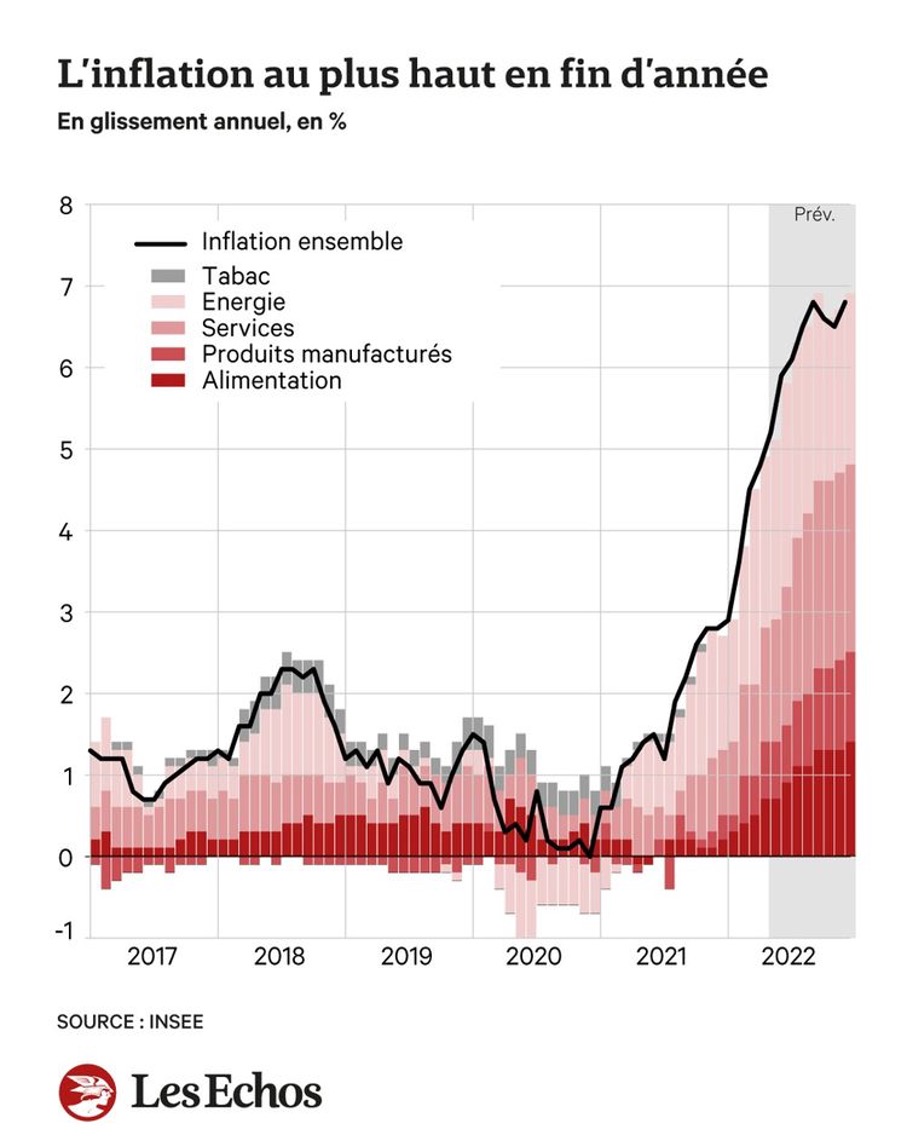
In the process of writing the report, I not only honed my analytical and presentation skills and learned to be graphic in the report, but also learned about the market situation of China’s home appliance industry. For example, I found that the two waves of the Covid pandemic in 2020 and 2022 showed different dynamics in terms of impact on the growth of demand for home appliances in China. The first wave of the pandemic increased the home cooking scenario; young consumers purchased basic, just-needed small appliances. The first wave of the pandemic led to an outbreak of live e-commerce, with online sales becoming the main channel for home appliance consumption, which drove rapid growth in demand for small appliances (like blenders and nutri-pots). The second wave of the pandemic has hampered logistics in some areas, and after 2020, the category of basic small home appliances was gradually saturated, and the demand was not fully released. The pandemic pushed consumers to form healthy living concepts and home cooking habits, demand shifted from basic appliances to advanced appliances. This pushed the industry product structure. So, I really felt the impact of the pandemic (a Black Swan) on the market in practice. For investors and companies, any major event means both challenges and opportunities.
Required skills and knowledge
When starting out, interns usually need to learn to write meeting minutes quickly and use Excel to do some simple calculations and data summaries. This is more of a test of the student’s information gathering skills and basic computer skills.
As we become familiar with the work, we need to apply our financial knowledge, understand industry dynamics, develop market insight and learn to express our opinions clearly. This includes being able to read company financial reports, fully analyze company operations, and make predictions about the future.
What I have learnt
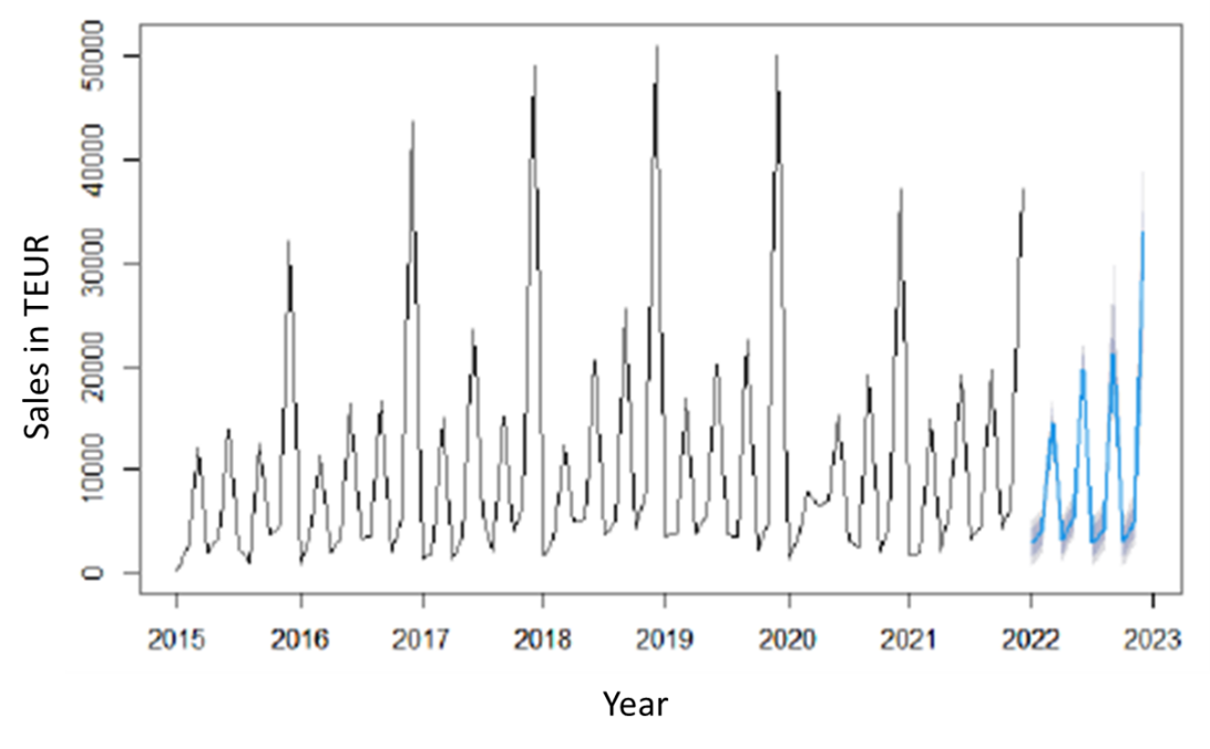
During my internship I worked with valuation models. Valuation modeling has always been an important section in company research or industry research reports. For investors, financial projections provide a visual representation of the underlying company’s operations and future state of development. Also, students looking for jobs in investment banks, equity research analyst firms and even consulting firms, need solid modeling skills.
The steps of valuation modeling financial projections are as follows:
- Forecast operating income and split revenue (different products and business, domestic vs foreign, etc.). Then forecast costs and expenses to complete the income statement forecast.
- Forecast the balance sheet and complete the forecast for all accounts except for the reserved matching items (money funds and financing gap).
- Prepare the cash flow statement, and calculate the monetary funds and financing gap on this basis.
- Fill in the vacant monetary funds and financing gap in the balance sheet, and match the balance sheet.
In fact, the complete financial modeling requires a lot of financial accounting knowledge and requires to be careful and conscientious, otherwise, the data can easily be wrong. On specific financial items, analysts need to mobilize financial knowledge to fill in the numbers. For example, depreciation and amortization are calculated with the fixed assets and intangible assets in the balance sheet forecast. Then we can go back to the income statement to fill in the two vacant cells. In the internship, I found that financial modeling is closely related to the financial management and financial statement courses we studied in university, so we still need to firmly grasp the basics of finance before seeking employment.
Key financial concepts
The discounted cash flow (DCF) model is a standard valuation method, which aims to calculate the value of a company based on the projected future cash flows of the company discounted to the present at the discount rate (weighted-average cost of capital or WACC).
Basic Formulas

Where EV means the enterprise value, FCF free cash flows, WACC the weighted-average cost of capital, and TV the terminal value.
Free Cash Flow
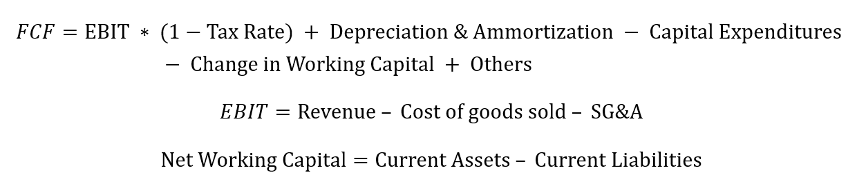
We can predict future turnover, expenses, tax rates, etc. by extrapolating the past or imagining the future of the company). Although this part of the formula is relatively complex, usually in practice the analysts will use the Excel formula or Visual Basic for Applications (VBA) to collate the various subjects, greatly simplifying the steps of financial modeling.
WACC

Where D represents the market value of the company’s debt, E the market value of equity capital, and t the income tax rate.
The Cost of equity can be calculated by CAPM model:

Where:
Risk free rate is the rate of return that can be obtained by investing money in an investment object without any risk.
β, also known as the beta coefficient, is a risk index that measures the price volatility of an individual stock or stock fund relative to the overall stock market.
Market risk premium, also known as equity risk premium or market risk return, refers to the difference between the return on a market portfolio and the risk-free rate of return. It measures the rate at which investors are paid for taking risk.
The Risk free rate can be the yield of the country’s national debt and β can be queried through the Wind database, such as the last three years of β.
Market risk premium is sometimes a forecast value in practice.
Cost of debt is the after-tax cost of debt. It is necessary to multiply the pre-tax cost by (1-t).
Terminal Value Calculation
To calculate the terminal value, we can use the Gordon Growth method to estimate the value based on its growth rate into perpetuity.
The Gordon Model, also known as the constant-growth model, is a special case of the dividend discount model, which reveals the relationship between the stock price, the expected base period dividend, the discount rate and the fixed growth rate of the dividend. The model has three assumptions:
1. The dividend payment is permanent in time;
2. The dividend growth rate is a constant;
3. The discount rate in the model is greater than the dividend growth rate.
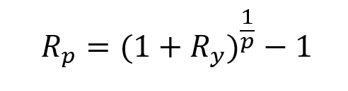
The terminal value is extrapolated from the Gordon model:
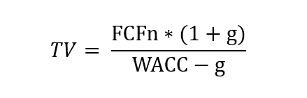
Where g is perpetual growth rate which means that the company has perpetual growth rate and return on invested capital. The perpetual growth model assumes stable and sustainable growth in the long term. In practice, g is usually a conservative figure.
Related posts on the SimTrade blog
▶ All posts about professional experiences
▶ Wenxuan HU My experience as an intern of the Wealth Management Department in Hwabao Securities
▶ Alexandre VERLET Classic brain teasers from real-life interviews
Useful resources
Industrial Securities
Wind Database
China Securities Regulatory Commission
About the author
The article was written in October 2022 by Wenxuan HU (ESSEC Business School, Global BBA, 2021-2023).