In this article, Youssef LOURAOUI (Bayes Business School, MSc. Energy, Trade & Finance, 2021-2022) elaborates on the concept of portfolio, which is a basic element in asset management.
This article is structured as follows: we introduce the concept of portfolio. We give the basic modelling to define and characterize a portfolio. We then expose the different types of portfolios that investors can rely on to meet their financial goals.
Introduction
An investment portfolio is a collection of assets that an investor owns. These assets can be individual assets such as bonds and stocks or baskets of assets such as mutual funds or exchange-traded funds (ETFs). In a nutshell, this refers to any asset that has the potential to increase in value or generate income. When building a portfolio, investors usually consider the expected return and risk. A well-balanced portfolio includes a variety of investments.
Modelling of portfolios
Portfolio weights
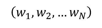
At a point of time, a portfolio is fully defined by the weights (w) of the assets of the universe considered (N assets).
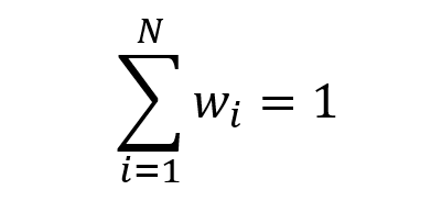
The sum of the portfolio weights adds up to one (or 100%):
The weight of a given asset i can be positive (for a long position in the asset), equal to zero (for a neutral position in the asset) or negative (for a short position in the asset):


Short selling is the process of selling a security without owning it. By definition, a short sell occurs when an investor borrows a stock, sells it, and then buys it later back to repay the lender.
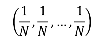
The equally-weighted portfolio is defined as the portfolio with weights that are evenly distributed across the number of assets held:
Portfolio return: the case of two assets
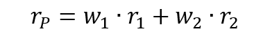
Over a given period of time, the returns on assets 1 and 2 are equal to r1 and r2. In the two-asset portfolio case, the portfolio return rP is computed as
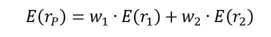
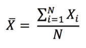
The expected return of the portfolio E(rP) is computed as
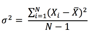
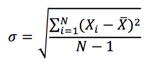
The standard deviation of the portfolio return, σ(rP) is computed as
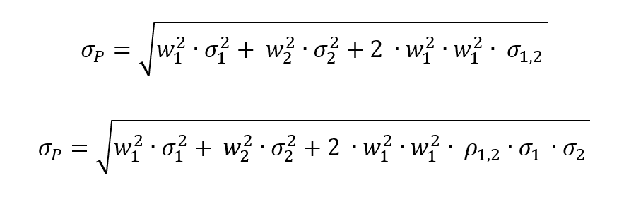
where:
- σ1 = standard deviation of asset 1
- σ2 = standard deviation of asset 2
- σ1,2 = covariance of assets 1 and 2
- ρ1,2 = correlation of assets 1 and 2
Investing in asset classes with low or no correlation to one another can help you increase portfolio diversification and reduce portfolio volatility. While diversification cannot guarantee a profit or eliminate the risk of investment loss, the ideal scenario is to have a mix of uncorrelated asset classes in order to reduce overall portfolio volatility and generate more consistent long-term returns. Correlation is depicted mathematically as the division of the covariance between the two assets by the individual standard deviation of the asset. Correlation is a more interpretable metric than covariance because it’s measurable within a defined rank. Correlation is measured between -1 and 1, with a high positive correlation showing that the assets move in tandem, while negative correlation depicts securities that have contrary price movements. The holy grail of investing is to invest in securities that offer a low correlation of the portfolio as a whole.
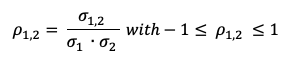
where:
- σ1,2 = covariance of assets 1 and 2
- σ1 = standard deviation of asset 1
- σ2 = standard deviation of asset 2
Correlation is a more interpretable metric than covariance because it’s measurable within a defined rank. Correlation is measured between -1 and 1, with high positive correlation showing that the assets move in tandem, while negative correlation depicts securities that have contrary price movements. The holy grail of investing is to invest in securities that offer a low correlation of the portfolio as a whole.
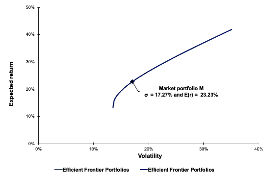
You can download an Excel file to help you construct a portfolio and compute the expected return and variance of a two-asset portfolio. Just introduce the inputs in the model and the calculations will be performed automatically. You can even draw the efficient frontier to plot the different combinations of portfolios that optimize the risk-return trade-off (to minimize the risk for a given level of expected return or to maximize the expected return for a given level of risk).

Portfolio return: the case of N assets
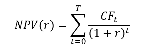
Over a given period of time, the return on asset i is equal to ri. The portfolio return can be computed as

The expression of the portfolio return is then used to compute two important portfolio characteristics for investors: the expected performance measured by the average return and the risk measured by the standard deviation of returns.
The expected return of the portfolio is given by
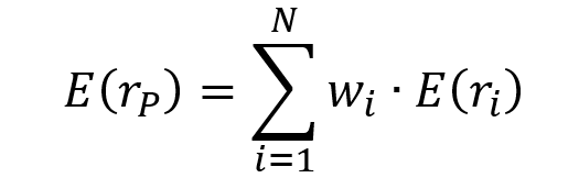
Because relying on multiple assets can get extremely computationally heavy, we can refer to the matrix form for more straightforward use. We basically compute the vector of weight with the vector of returns (NB: we have to pay attention to the dimension and to the properties of matrix algebra).
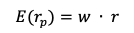
- w = weight vector
- r = returns vector
The standard deviation of returns of the portfolio is given by the following equivalent formulas:
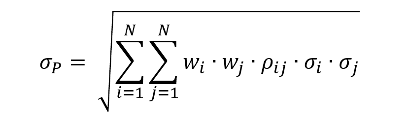
- wi = weight of asset i
- wj = weight of asset j
- σi = standard deviation of asset i
- σj = standard deviation of asset j
- ρi,j = correlation of asset i,j
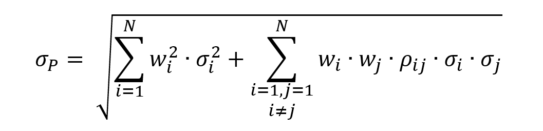
where:
- wi2 = squared weight of asset I
- σi2 = variance of asset i
- wi = weight of asset i
- wj = weight of asset j
- σi = standard deviation of asset i
- σj = standard deviation of asset j
- ρi,j = correlation of asset i,j
We can use the matrix form for a more straightforward application due to the computational burden associated with relying on multiple assets. Essentially, we multiply the vector of weights with the variance-covariance matrix and the transposed weight vector (NB: we must pay attention to the dimension and to the properties of matrix algebra).
- w = weight vector
- ∑ = variance-covariance matrix
- w’ = transpose of weight vector
You can get an Excel file that will help you build a portfolio and calculate the expected return and variance of a three-asset portfolio. Simply enter the data into the model, and the calculations will be carried out automatically. You can even use the efficient frontier to plot the various portfolio combinations that best balance risk and reward (to minimize the risk for a given level of expected return or to maximize the expected return for a given level of risk).
Basic principles on portfolio construction
Diversify
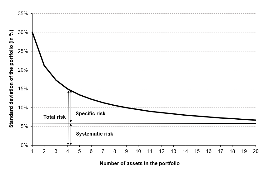
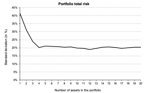
Diversification, a core principle of Markowitz’s portfolio selection theory, is a risk-reduction strategy that entails allocating assets among a variety of financial instruments, sectors, and other asset classes (Markowitz, 1952). In more straightforward terms, it refers to the concept “don’t put all your eggs in one basket.” If the basket is dropped, all eggs are shattered; if many baskets are used, the likelihood of all eggs being destroyed is significantly decreased. Diversification may be accomplished by investments in a variety of companies, asset types (e.g., bonds, real estate, etc.), and/or commodities such as gold or oil.
Diversification seeks to enhance returns while minimizing risk by investing in a variety of assets that will react differently to the same event(s). Portfolio diversification methods should include not just diverse stocks inside and outside of the same industry, but also diverse asset classes, such as bonds and commodities. When there is an imperfect connection between assets (lower than one), the diversification effect occurs. It is a critical and successful risk mitigation method since risk mitigation may be accomplished without jeopardizing profits. As a result, any prudent investor who is cautious (or ‘risk averse’) will diversify to a certain extent.
Portfolio Asset Allocation
The term “asset allocation” refers to the proportion of stocks, bonds, and cash in a portfolio. Depending on your investing strategy, you’ll determine the percentage of each asset type in your portfolio to achieve your objectives. As markets fluctuate over time, your asset allocation is likely to go out of balance. For instance, if Tesla’s stock price increases, the percentage of your portfolio allocated to stocks will almost certainly increase as well.
Portfolio Rebalancing
Rebalancing is a term that refers to the act of purchasing and selling assets in order to restore your portfolio’s asset allocation to its original state and avoid disrupting your plan.
Reduce investment costs as much as possible
Commission fees and management costs are significant expenses for investors. This is especially important if you frequently purchase and sell stocks. Consider using a discount brokerage business to make your investment. Clients are charged much lesser fees by these firms. Also, when investing for the long run, it is advisable to avoid making judgments based on short-term market fluctuations. To put it another way, don’t sell your stocks just because they’ve taken a minor downturn in the near term.
Invest on a regular basis
It is critical to invest on a regular basis in order to strengthen your portfolio. This will not only build wealth over time, but it will also develop the habit of investing discipline.
Buying in the future
It’s possible that you have no idea how a new stock will perform when you buy it. To be on the safe side, avoid putting your entire position to a single investment. Start with a little investment in the stock. If the stock’s performance fulfils your expectations, you can gradually increase your investments until you’ve covered your entire position.
Types of portfolio
We detail below the different types of portfolios usually proposed by financial institutions that investors can rely on to meet their financial goals.
Aggressive Portfolio
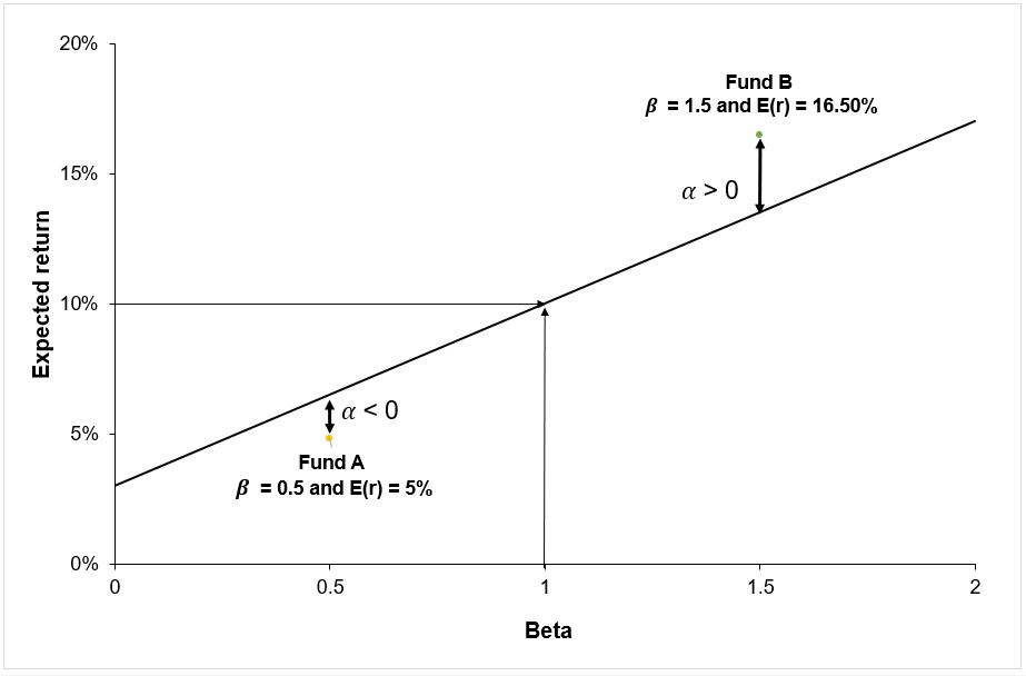
As the name implies, an aggressive portfolio is one of the most frequent types of portfolio that takes a higher risk in the pursuit of higher returns. Stocks in an aggressive portfolio have a high beta, which means they present more price fluctuations compared to the market. It is critical to manage risk carefully in this type of portfolio. Keeping losses to a minimal and taking profits are crucial to success. It is suitable for a high-risk appetite investor.
Defensive Portfolio
A defensive portfolio is one that consists of stocks with a low beta. The stocks in this portfolio are largely immune to market swings. The goal of this type of portfolio is to reduce the risk of losing the principal. Fixed-income securities typically make up a major component of a defensive portfolio. It is suitable for a low-risk appetite investor.
Income Portfolio
Another typical portfolio type is one that focuses on investments that generate income from dividends (for stocks), interests (for bonds) or rents (for real estate). An income portfolio invests in companies that return a portion of their profits to shareholders, generating positive cash flow. It is critical to remember that the performance of stocks in an income portfolio is influenced by the current economic condition.
Speculative Portfolio
Among all portfolio types, a speculative portfolio has the biggest risk. Speculative investments could be made of different assets that possess inherently higher risks. Stocks from technology and health-care companies that are developing a breakthrough product, junk bonds, distressed investments among others might potentially be included in a speculative portfolio. When establishing a speculative portfolio, investors must exercise caution due to the high risk involved.
Hybrid Portfolio
A hybrid portfolio is one that includes passive investments and offers a lot of flexibility. The cornerstone of a hybrid portfolio is typically made up of blue-chip stocks and high-grade corporate or government bonds. A hybrid portfolio provides diversity across many asset classes while also providing stability by combining stocks and bonds in a predetermined proportion.
Socially Responsible Portfolio
A socially responsible portfolio is based on environmental, social, and governance (ESG) criteria. It allows investors to make money while also doing good for society. Socially responsible or ESG portfolios can be structured for any level of risk or investment aim and can be built for growth or asset preservation. The important thing is that they prefer stocks and bonds that aim to reduce or eliminate environmental impact or promote diversity and equality.
Why should I be interested in this post?
Portfolio management’s objective is to optimize the returns on the entire portfolio, not just on one or two stocks. By monitoring and maintaining your investment portfolio, you can accumulate a sizable capital to fulfil a variety of financial objectives, including retirement planning. This article helps to understand the grounding fundamentals behind portfolio construction and investing.
Related posts on the SimTrade blog
▶ Youssef LOURAOUI Markowitz Modern Portfolio Theory
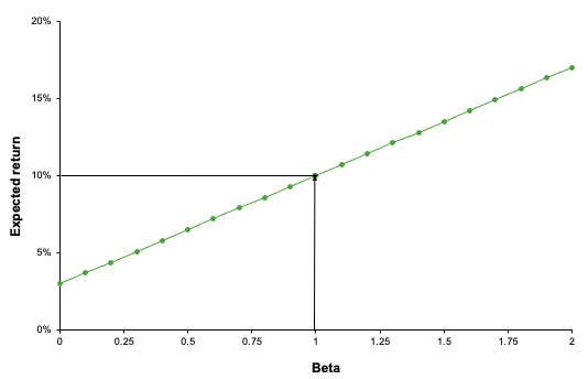
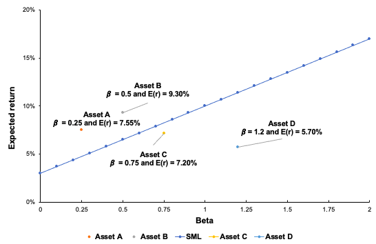
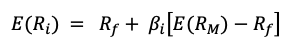
▶ Jayati WALIA Capital Asset Pricing Model (CAPM)
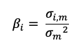
▶ Youssef LOURAOUI Beta
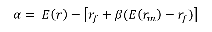
▶ Youssef LOURAOUI Alpha
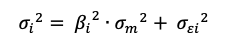
▶ Youssef LOURAOUI Systematic and specific risk
▶ Jayati WALIA Value at Risk (VaR)
▶ Anant JAIN Social Responsible Investing (SRI)
Useful resources
Academic research
Mangram, M.E., 2013. A simplified perspective of the Markowitz Portfolio Theory. Global Journal of Business Research, 7(1): 59-70.
Markowitz, H., 1952. Portfolio Selection. The Journal of Finance, 7(1): 77-91.
Business analysis
Edelweiss, 2021.What is a portfolio?
Forbes, 2021.Investing basics: What is a portfolio?
JP Morgan Asset Management, 2021.Glossary of investment terms: Portfolio
About the author
The article was written in November 2021 by Youssef LOURAOUI (Bayes Business School, MSc. Energy, Trade & Finance, 2021-2022).


 .
.


 Source: Computations from the author.
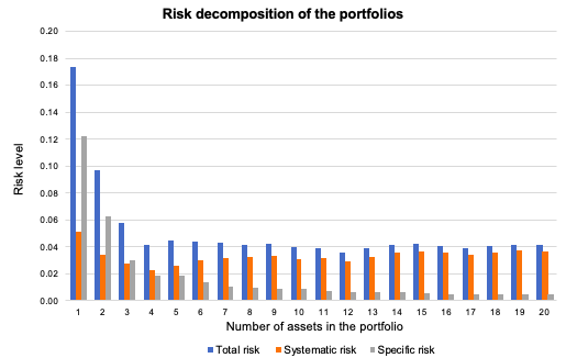 Source: Computations from the author.
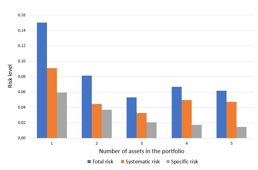 Source: Computation from the author.
 Source: Computation from the author.