Barrier options

In this article, Shengyu ZHENG (ESSEC Business School, Grande Ecole Program – Master in Management, 2020-2023) explains barrier options which are the most traded exotic options in derivatives markets.
Description
Barrier options are path dependent. Their payoffs are not only a function of the price of the underlying asset relative to the option strike, but also depend on whether the price of the underlying asset reached a certain predefined barrier during the life of the option.
The two most common kinds of barrier options are knock-in (KI) and knock-out (KO) options.
Knock-in (KI) barrier options
KI barrier options are options that are activated only if the underlying asset attains a prespecified barrier level (the “knock-in” event). With the absence of this knock-in event, the payoff remains zero regardless of the trajectory of the price of the underlying asset.
Knock-out (KO) barrier options
KO barrier options are options that are deactivated only if the underlying asset attains a prespecified barrier level (the “knock-out” event). In the presence of this knock-out event, the payoff remains zero regardless of the trajectory of the price of the underlying asset.
Observation
The determination of the occurrence of a barrier event (KI or KO conditions) is essential to the ultimate payoff of the barrier option. In practice, the details of the KI or KO conditions are precisely defined in the contract (called “Confirmations” by the International Swaps and Derivatives Association (ISDA) for over-the counter (OTC) traded options).
Observation period
The observation period denotes the period where a barrier event (KI or KO) can be observed, that is to say, when the price of the underlying asset is monitored. There are three styles of observation period: European style, partial-period American style, and full-period American style.
- European style: The observation period is only the expiration date of the barrier option.
- Partial-period American style: The observation period is part of the lifespan of the barrier option.
- Full-period American style: The observation period spans the whole period from the effective date to the expiration date of the barrier option.
Monitoring method
There are two typical types of monitoring methods in terms of the determination of a knock-in/knock-out event: continuous monitoring and discrete monitoring. The monitoring method is one of the key factors in determining the premium of a barrier option.
- Continuous monitoring: A knock-in/knock-out event is deemed to take place if, at any time in the observation period, the knock-in/knock-out condition is met.
- Discrete monitoring: A knock-in/knock-out event is deemed to occur if, at pre-specific times in the observation period, usually the closing time of each trading day, the knock-in/knock-out condition is met.
Barrier Reference Asset
For the most cases, the Barrier Reference Asset is the underlying asset itself. However, if specified in the contract, it can be another asset or index. It can also be other calculatable properties, such as the volatility of the asset. In this case, the methodology of calculating such properties should be clearly defined in the contract.
Rebate
For knock-out options, there could be a rebate. A rebate is an extra feature and it corresponds to the amount that should be paid to the buyer of the knock-out option in case of the occurrence of a knock-out event.
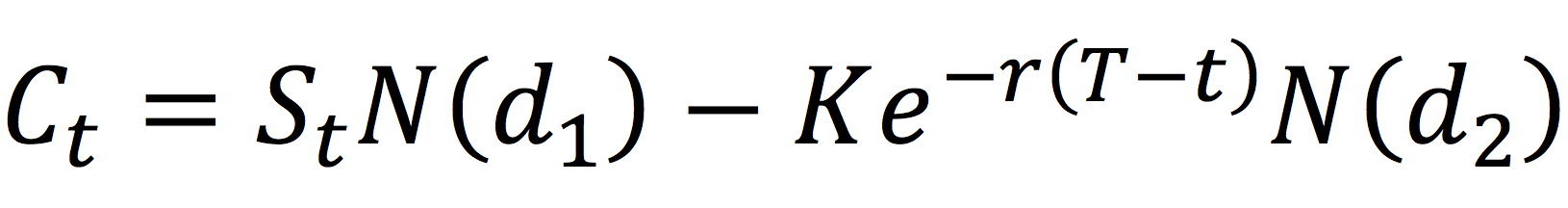
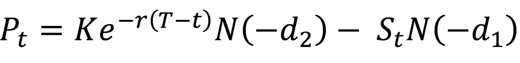
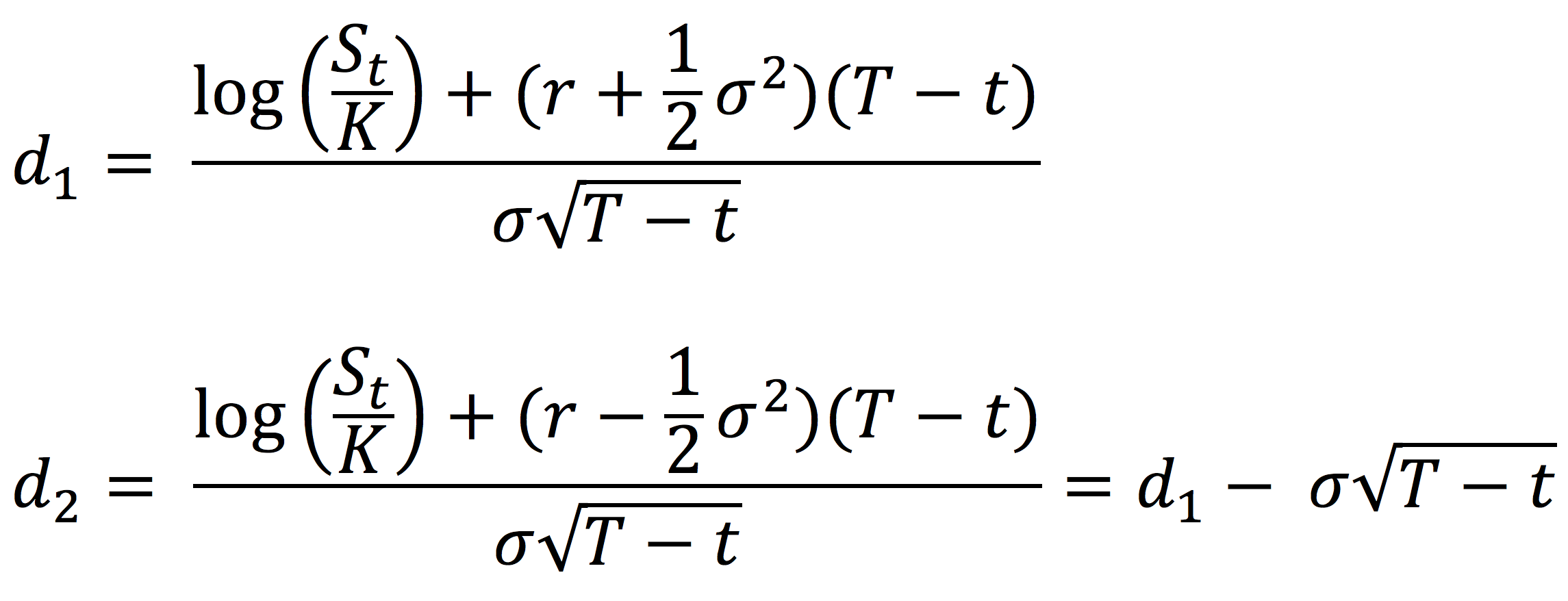
In-out parity relation for barrier options
Analogous to the call-put parity relation for plain vanilla options, there is an in-out parity relation for barrier options stating that a long position in a knock-in option plus a long position in a knock-out option with identical strikes, barriers, monitoring methods and maturity is equivalent to a long position in a comparable vanilla option. It could be stated as follows:
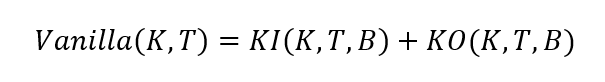
Where K denotes the strike price, T the maturity, and B the barrier level.
It is worth noting that this parity relation is valid only when the two KI and KO options are identical, and there is no rebate in case of a knock-out option.
Basic barrier options
There are four types of basic barrier options traded in the market: up-and-in option, up-and-out option, down-and-in option, and down-and-out option. “Up” and “down” denotes the direction of surpassing the barrier price. “In” and “out” depict the type of barrier condition, i.e. knock-in or knock-out. These four types of barrier features are available for both call and put options.
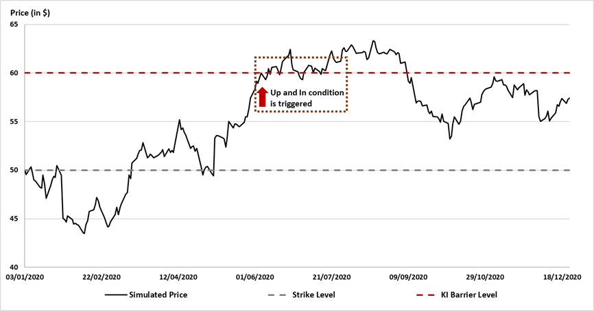
Up-and-in option
An up-and-in option is a knock-in option whose barrier condition is achieved if the underlying price arrives higher than the barrier level during the observation period.
Figure 1 illustrates the occurrence of an up-and-in barrier event for a barrier option with full-period American style and discrete monitoring (the closing time of each trading day).
Figure 1. Illustration of an up-and-in barrier option
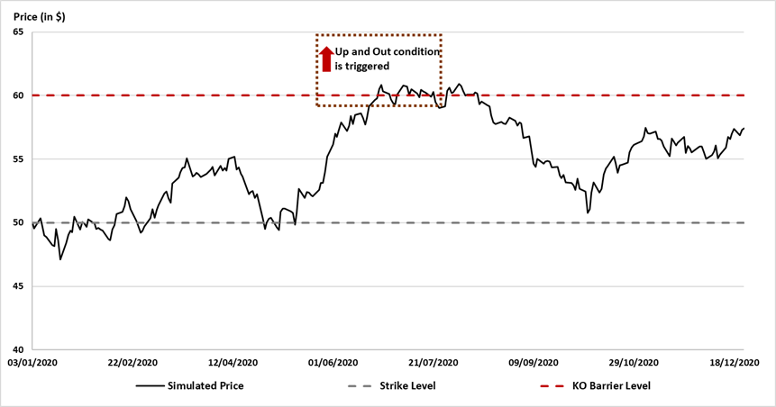
Up-and-out option
An up-and-out option is a knock-out option whose barrier condition is achieved if the underlying price arrives higher than the barrier level during the observation period.
Figure 2. Illustration of an up-and-out option
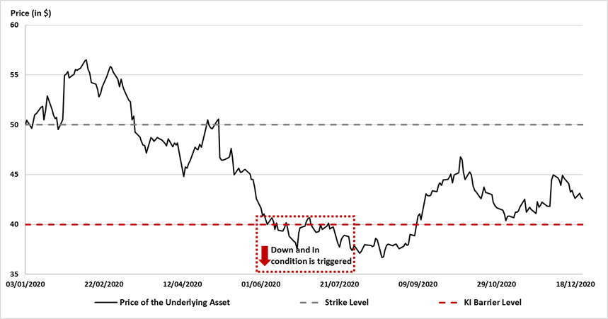
Down-and-in option
A down-and-in option is a knock-in option whose barrier condition is achieved if the underlying price arrives lower than the barrier level during the observation period.
Figure 3. Illustration of a down-and-in option
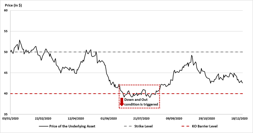
Down-and-out option
A down-and-out option is a knock-out option whose barrier condition is achieved if the underlying price arrives lower than the barrier level during the observation period.
Figure 4. Illustration of a down-and-out option
Download R file to price barrier options
You can find below an R file to price barrier options.

Trading of barrier options
Being the most popular exotic options, barrier options on stocks or indices have been actively traded in the OTC market since the inception of the market. Unavailable in standard exchanges, they are less accessible than their vanilla counterparts. Barrier options are also commonly utilized in structured products.
Why should I be interested in this post?
As one of the most traded but the simplest exotic derivative products, barrier options open an avenue for different applications. They are also very often incorporated in structured products, such as reverse convertibles. Knock-in/knock out conditions are also common features in other types of more complicated exotic derivative products.
It is, therefore, important to be equipped with knowledge of this product and to understand the pricing logics if one aspires to work in financial markets.
Related posts on the SimTrade blog
▶ Shengyu ZHENG Pricing barrier options with analytical formulas
▶ Shengyu ZHENG Pricing barrier options with simulations and sensitivity analysis with Greeks
References
Academic research articles
Broadie, M., Glasserman P., Kou S. (1997) A Continuity Correction for Discrete Barrier Option. Mathematical Finance, 7:325-349.
Merton, R. (1973) Theory of Rational Option Pricing. The Bell Journal of Economics and Management Science, 4:141-183.
Paixao, T. (2012) A Guide to Structured Products – Reverse Convertible on S&P500
Reiner, E.S., Rubinstein, M. (1991) Breaking down the barriers. Risk Magazine, 4(8), 28–35.
Rich, D. R. (1994) The Mathematical Foundations of Barrier Option-Pricing Theory. Advances in Futures and Options Research: A Research Annual, 7:267-311.
Wang, B., Wang, L. (2011) Pricing Barrier Options using Monte Carlo Methods, Working paper.
Books
Haug, E. (1997) The Complete Guide to Option Pricing. London/New York: McGraw-Hill.
Hull, J. (2006) Options, Futures, and Other Derivatives. Upper Saddle River, N.J: Pearson/Prentice Hall.
About the author
The article was written in July 2022 by Shengyu ZHENG (ESSEC Business School, Grande Ecole Program – Master in Management, 2020-2023).

 Source : computation by the author.
 Source: computation by the author.