
In this article, Youssef LOURAOUI (Bayes Business School, MSc. Energy, Trade & Finance, 2021-2022) presents the Fama-MacBeth regression method used to test asset pricing models and addresses the difference when applying the regression method on individual stocks or portfolios composed of stocks with similar betas.
This article is structured as follow: we introduce the Fama-MacBeth testing method. Then, we present the mathematical foundation that underpins their approach. We conduct an empirical analysis on both the stock and the portfolio approach. We conclude with a discussion on econometric issues.
Introduction
Risk factors are frequently employed to explain asset returns in asset pricing theories. These risk factors may be macroeconomic (such as consumer inflation or unemployment) or microeconomic (such as firm size or various accounting and financial metrics of the firms). The Fama-MacBeth two-step regression approach found a practical way for measuring how correctly these risk factors explain asset or portfolio returns. The aim of the model is to determine the risk premium associated with the exposure to these risk factors.
As a reminder, the Fama-MacBeth regression method is composed on two steps: step 1 with a time-series regression and step 2 with a cross-section regression.
The first step is to regress the return of every stock against one or more risk factors using a time-series regression. We obtain the return exposure to each factor called the “betas” or the “factor exposures” or the “factor loadings”.
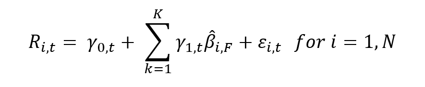
The second step is to regress the returns of all stocks against the asset betas obtained in the first step using a cross-section regression for different periods. We obtain the risk premium for each factor used to test the asset pricing model.
The implementation of this method can be done with individual stocks or with portfolios of stocks as proposed by Fama and MacBeth (1973). Their argument is the better stability of the beta when considering portfolios. In this article we illustrate the difference with the two implementations.
Fama and MacBeth (1973) implemented with individual stocks
We downloaded a sample of daily prices of stocks composing the S&P500 index over the period from January 03, 2012, to December 31, 2021 (we selected the stocks present from the beginning to the end of the period reducing our sample from 500 to 440 stocks). We computed daily returns for each stock and for the market factor retained in this study. To represent the market, we chose the S&P500 index, an important global stock benchmark capturing the US equity market.
The procedure to derive the Fama-MacBeth regression using the stock approach can be achieved as follow:
Step 1: time-series regression
We compute the beta of the stocks with respect to the market factor for the period covered (time-series regression). We estimate the beta of each stock related to the S&P500 index. The beta is computed as the slope of the linear regression of the stock return on the market return (S&P500 index return). This time-series regression is run on a subperiod of the whole period from January 03, 2012, to December 31, 2018.
Step 2: cross-sectional regression
Over a second period from January 04, 2019, to December 31, 2021, we compute the dynamic regression of returns at each data point in time with respect to the betas computed in Step 1.
With this procedure, we obtain a risk premium that would represent the relationship between the stock returns at each data point in time with their respective beta for the sample analyzed.
Test the statistical significance of the results obtained from the regression
Results in the time-series regression using the stock approach are statistically significant. As shown in Table 1, the p-value is in the rejection area, which implies that the factor that the market factor can be considered as a driver of return.
Table 1. Time-series regression t-statistic result.
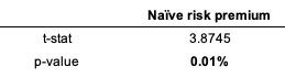 Source: computation by the author.
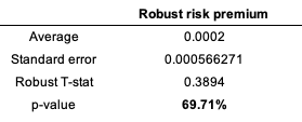
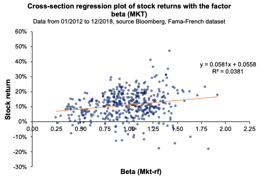
However, when analyzed in the cross-section regression, the results are not statistically significant anymore. As shown in Table 2, the p-value is not in the rejection area. We cannot reject the null hypothesis (H0: non significance of the market factor). Market factor alone cannot explain the premium investors are considering.
This means that the market factor fails to explain properly the behavior of asset returns, which undermines the validity of the CAPM framework. These results are in line with the Fama-MacBeth paper (1973).
Table 2. Cross-section regression t-statistic result.
 Source: computation by the author.
You can find below the Excel spreadsheet that complements the explanations covered in this part of the article (implementation of the Fama and MacBeth (1973) method with individual stocks).

Fama and MacBeth (1973) implemented with portfolios of stocks
Fama-MacBeth seminal paper (1973) was based on an analysis of the market factor by assessing constructed portfolios of similar betas ranked by increasing values. This approach helped to overcome the shortcoming regarding the stability of the beta and correct for conditional heteroscedasticity derived from the computation of the betas for individual stocks. They performed a second time the cross-sectional regression of monthly portfolio returns based on equity betas to account for the dynamic nature of stock returns, which help to compute a robust standard error and assess if there is any heteroscedasticity in the regression. The conclusion of the seminal paper suggests that the beta is “dead”, in the sense that it cannot explain returns on its own (Fama and MacBeth, 1973).
The procedure to derive the Fama-MacBeth regression using the portfolio approach can be achieved as follow:
Step 1: time-series regression
We first compute the beta of the stocks with respect to the market factor for the period covered (time-series regression). We estimate the beta of each stock related to the S&P500 index. The beta is computed as the slope of the linear regression of the stock return on the market return (S&P500 index return). This time-series regression is run on a subperiod of the whole period from January 03, 2012, to December 31, 2015. We build twenty portfolios based on stock betas ranked in ascending order. The betas of the portfolios are then estimated again on a subperiod from January 04, 2016, to December 31, 2018.
It is challenging to maintain beta stability over time. Fama-MacBeth aimed to remedy this shortcoming through its novel technique. However, some issues must be addressed. When betas are calculated using a monthly time series, the statistical noise in the time series is significantly reduced in comparison to shorter time frames (i.e., daily observation). When portfolio betas are constructed, the coefficient becomes considerably more stable than when individual betas are evaluated. This is due to the diversification impact that a portfolio can produce, which considerably reduces the amount of specific risk.
Step 2: cross-sectional regression
Over a second period from January 03, 2019, to December 31, 2021, we compute the dynamic regression of portfolio returns at each data point in time with respect to the betas computed in Step 1.
With this procedure, we obtain a risk premium that would represent the relationship between the portfolio returns at each data point in time with their respective beta for the sample analyzed.
Test the statistical significance of the results obtained from the regression
Results in the cross-section regression using the portfolio approach are not statistically significant. As captured in Table 3, the p-value is not in the rejection area, which implies that the factor is statistically insignificant and that the market factor cannot be considered as a driver of return.
Table 3. Cross-section regression with portfolio approach t-statistic result.
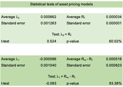 Source: computation by the author.
You can find below the Excel spreadsheet that complements the explanations covered in this part of the article (implementation of the Fama and MacBeth (1973) method with portfolios of stocks).
Econometric issues
Errors in data measurement
Because regression uses a sample instead of the entire population, a certain margin of error must be accounted for since the authors derive estimated betas for the sample.
Asset return heteroscedasticity
In econometrics, heteroscedasticity is an important concern since it results in unequal residual variance. This indicates that a time series exhibiting some heteroscedasticity has a non-constant variance, which renders forecasting ineffective because the time series will not revert to its long-run mean.
Asset return autocorrelation
Standard errors in Fama-MacBeth regressions are solely corrected for cross-sectional correlation. This method does not fix the standard errors for time-series autocorrelation. This is typically not a concern for stock trading, as daily and weekly holding periods have modest time-series autocorrelation, whereas autocorrelation is larger over long horizons. This suggests that Fama-MacBeth regression may not be applicable in many corporate finance contexts where project holding durations are typically lengthy.
Why should I be interested in this post?
Fama-MacBeth made a significant contribution to the field of econometrics. Their findings cleared the way for asset pricing theory to gain traction in academic literature. The Capital Asset Pricing Model (CAPM) is far too simplistic for a real-world scenario since the market factor is not the only source that drives returns; asset return is generated from a range of factors, each of which influences the overall return. This framework helps in capturing other sources of return.
Related posts on the SimTrade blog
▶ Youssef LOURAOUI Fama-MacBeth regression method: N-factors application
▶ Youssef LOURAOUI Fama-MacBeth regression method: Analysis of the market factor
▶ Jayati WALIA Capital Asset Pricing Model (CAPM)
▶ Youssef LOURAOUI Security Market Line (SML)
▶ Youssef LOURAOUI Origin of factor investing
▶ Youssef LOURAOUI Factor Investing
Useful resources
Academic research
Brooks, C., 2019. Introductory Econometrics for Finance (4th ed.). Cambridge: Cambridge University Press. doi:10.1017/9781108524872
Fama, E. F., MacBeth, J. D., 1973. Risk, Return, and Equilibrium: Empirical Tests. Journal of Political Economy, 81(3), 607–636.
Roll R., 1977. A critique of the Asset Pricing Theory’s test, Part I: On Past and Potential Testability of the Theory. Journal of Financial Economics, 1, 129-176.
American Finance Association & Journal of Finance (2008) Masters of Finance: Eugene Fama (YouTube video)
About the author
The article was written in December 2022 by Youssef LOURAOUI (Bayes Business School, MSc. Energy, Trade & Finance, 2021-2022).


 Source: computation by the author.
 Source: computation by the author.
 Source: computation by the author.
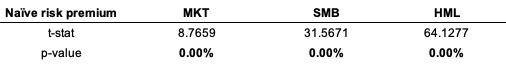 Source: computation by the author.
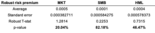 Source: computation by the author.