Smart Beta strategies: between active and passive allocation

In this article, Youssef LOURAOUI (ESSEC Business School, Global Bachelor of Business Administration, 2017-2021) discusses the topic of smart beta strategies and especially the debate about its position as an active or passive allocation.
Smart beta strategies appear to be in the middle of the polarized asset management industry, which is segmented between active investing based on beating the performance of a given benchmark, and passive investing based on replicating a given benchmark.
This article is structured as follows: we begin by introducing the topic of smart beta strategies. We then discuss the different investing approach and their characteristic. A simple simulation exercise is then presented to understand how an alternative to market-capitalization-weightings indexes leads to different results. We wrap up with a general conclusion of the topic.
Introduction
Smart beta strategies are often found somewhere in the middle between active and passive investment management. In this post, we look at how investors think about this characteristic of smart beta investment strategies.
Passive funds aim at replicating or tracking an index (such as the S&P500 index in the US or the CAC40 index in France for equity markets) use a buy-and-hold strategy to achieve their goal of mimicking the performance of the market index. The beta of a passive fund is very close to the beta of the market index (benchmark).
Active funds are supervised by a portfolio manager that screens the best investments for the fund and time the market to profit from an upside potential. The excess return over the performance of the market index (benchmark) is referred to as alpha.
Smart beta funds are justified by the fact that capitalization-weighted strategies appear to be inefficient. They are based on transparent and rule-based strategies. Investors seek to obtain additional factor betas to enhance their portfolio performance.
While passive investing aims to match the market return, and active strategies rely on the fund manager’s ability to outperform the market, smart beta can be seen as a hybrid of the two approaches, with a passive component in the sense that it tracks one or more factors that are transparent and rule-based, and an active component in which the portfolio is managed, that is to say, rebalanced from time to time. Table 1 describes the main types of funds (passive, active and smart beta) and their respective strategies according to the investment approach and asset allocation methodology, and performance metrics. We also indicate the Greek letter that each strategy.
Table 1. Description of the main types of funds and their respective strategies.
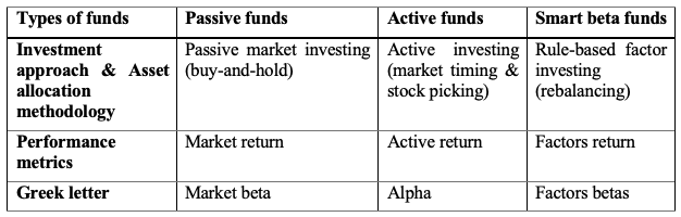
Source: table done by the author.
The passive investing approach
The Efficient Market Hypothesis (EMH) asserts that markets are efficient. The passive investing strategy is built on the concept of “buy-and-hold,” or keeping an investment position for a lengthy period without worrying about market timing or acting on the bought position. This latter technique is frequently implemented through the purchase of exchange-traded funds (ETF) that aim to closely match a given benchmark to produce a performance that is comparable to the underlying index or benchmark. The index might be broad-based, such as the S&P500 index in the US equity market for instance, or more specialized, such as an index that monitors a specific sector or geographical zone.
The active investing approach
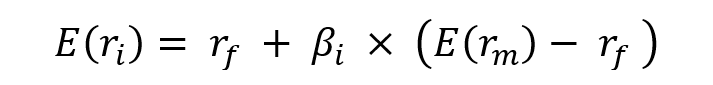
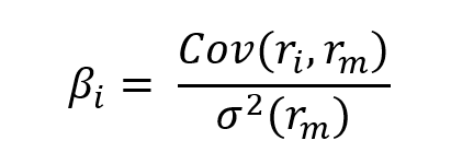
Active management is an approach for going beyond matching a benchmark’s performance and instead aiming to outperform it. The alpha may be calculated using the same CAPM model framework, by linking the expected return with the fund manager’s extra return on the portfolio’s overall performance (Jensen, 1968). The search for alpha is done through two very different types of investment approaches: stock picking and market timing.
Stock picking
Stock picking is a method used by active managers to select assets based on a variety of variables such as their intrinsic value, the growth rate of dividends, and so on. Active managers use the fundamental analysis approach, which is based on the dissection of economic and financial data that may impact the asset price in the market.
Market timing
Market timing is a trading approach that involves entering and exiting the market at the right time. In other words, when rising outlooks are expected, investors will enter the market, and when downward outlooks are expected, investors will exit. For instance, technical analysis, which examines price and volume of transactions over time to forecast short-term future evolution, and fundamental analysis, which examines the macroeconomic and microeconomic data to forecast future asset prices, are the two techniques on which active managers base their decisions.
Review of academic literature
Passive investing
We can retrace the foundations of passive investing to the theory of portfolio construction developed by Harry Markowitz. For his theoretical implications, Markowitz’s work is widely regarded as a pioneer in financial economics and corporate finance. For his contributions to these disciplines, which he developed in his thesis “Portfolio Selection” published in The Journal of Finance in 1952. Markowitz received the Nobel Prize in economics in 1990. His groundbreaking work set the foundation for what is now known as ‘Modern Portfolio Theory’ (MPT).
William Sharpe, John Lintner, and Jan Mossin separately developed The Capital Asset Pricing Model (CAPM) as a result of Markowitz past research. The CAPM was a huge evolutionary step forward in capital market equilibrium theory because it enabled investors to appropriately value assets in terms of systematic risk. The portfolio management industry intended to capture the market portfolio return in the late 1970s, defined as a hypothetical collection of investments that contains every kind of asset available in the investment universe, with each asset weighted in proportion to its overall market participation. A market portfolio’s expected return is the same as the market’s overall expected return. But as financial research evolved and some substantial contributions were made, new factor characteristics emerged to capture some additional performance.
Active investing
As fund managers tried strategies to beat the market, financial literature delved deeper into the mechanism to achieve this purpose. Jensen’s groundbreaking work in the early ’70s gave rise to the concept of alpha in the tracking of a fund’s performance to distinguish between the fund’s manager’s ability to generate abnormal returns and the part of the returns due to luck (Jensen, 1968).
Smart beta / factor investing
Smart beta is defined as strategies that aim to address the inefficiencies of market capitalization weight indexation. In the early 2000s, as a result of numerous financial publications delving deeper into various elements that gave additional returns to increase the overall performance of the portfolio (the “Fama-French” papers), smart beta strategies evolved. Fund managers develop investment strategies based on researched factors that provide a time-tested abnormal return in exchange for taking on risk.
Understanding portfolio returns is crucial to determining how to evaluate portfolio performance. It all stems from Harry Markowitz’s groundbreaking work and pioneering research on portfolio construction and the impact of diversification in improving portfolio performance. Throughout the 1960s and 1970s, investors made no distinction between the sources of portfolio returns. Finance research in the 1980s boosted the popularity of passive investment as an alternate basis for implementation. Investors began to successfully capture market beta through passive strategies. In the 2000s, investors began to see factors as major determinants of long-term return (Figure 1).
Figure 1. Overview of the evolution of performance metrics.
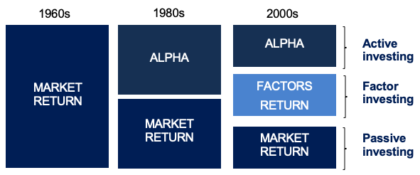
Source: MSCI Factor Research (2021).
Grossman and Stiglitz’s research addressed the limitations of passive investment (1980). If the fund manager actively selects assets for his portfolio rather than passively replicating the benchmark, he may get higher abnormal returns. The term “abnormal returns” refers to the disparity between the actual and projected returns. In the financial literature, this “extra return” is referred to as alpha. It is one of the most tracked performance indicators by fund managers. Grossman and Stiglitz establish that there is no such thing as a successful passive investment. Indeed, they said that the benchmark is composed of assets chosen based on certain criteria (capitalization, return, liquidity, and the weight of each asset in the sector), and that “passive investing” is the most cost-effective alternative to active investing.
As pointed out by Jensen (1968), when assembling a portfolio, there are two points to bear in mind. The first point is the fund manager’s ability to foresee the asset’s price movement, and the second point is the fund manager’s capacity to limit investment risk via diversification.
Case study: Comparison of market-capitalization-weighted portfolios and equally-weighted portfolios
The difference between two investment strategies can be evaluated by comparing the weights of the assets of their associated portfolio. Note that over time the weights can evolve with voluntary sales and purchases of the assets. Such divestments and investments refer to the rebalancing of the portfolio.
Buy-and-hold investing is a passive investment strategy in which an investor buys assets and holds them for a long period, independent of market fluctuations. A buy-and-hold investor selects companies but is indifferent to short-term market swings or technical indicators. The buy-and-hold investment strategy corresponds to market-capitalization-weighted portfolios.
The buy-and-hold approach is recommended by several prominent investors, like Warren Buffett, to individuals seeking profitable long-term returns. Buy-and-hold investors outperform active management on average over longer time horizons and after costs. Buy-and-hold investors, on the other hand, may not sell at the greatest price available, according to proponents.
Excel file for market-capitalization-weighted and equally-weighted portfolios
You can download an Excel file with data used for this exercise.

The goal of this exercise is to compare the performance of the two types of investments and to balance the two approaches to obtain a better understanding of each strategy and its market behavior. To be able to homogeneously analyze the underlying assets of the buy and hold strategy as well as the smart beta approach, three stocks have been simulated.
All the price data, number of shares, stock returns, and market-capitalization are all simulated for a more simplistic model. The buy and hold strategy is based on an evenly weighted portfolio. Only the small-cap stock (Stock 1) will have prices fluctuations to analyze the size effect as a driver of returns in a portfolio. A rebalancing exercise is implemented for the smart beta portfolio, no trading nor any related cost for implementing the strategy is applied and thus, don’t reflect the full picture as in financial markets.
Table 2 is made of three components. The first section of the table represents our data for the simulation. Each stock has a different size representing respectively a small, mid, and large-capitalization firm. Market capitalization is obtained through a simple computation by multiplying the number of shares times the price of each share. The second section of the table is the simulation of a market-capitalization-weighted portfolio. The third section represents a smart beta portfolio that uses an equally-weighted weighting indexing (Table 2). Note that with the market-capitalization-weighted portfolio there is a concentration in the stock with the largest market capitalization (due to its high past performance). An equally-weighted portfolio obtained with rebalancing (often associated with smart beta strategies such as growth) would not present such property and show a more diversified portfolio over time. Note that the frequency of rebalancing the portfolio can affect the risk/performance characteristics. Amenc et. al. (2016) show that the Sharpe ratio tends to decrease with a higher frequency for rebalancing.
Table 2. Simulation of a market-capitalization-weighted portfolio and an equally-weighted portfolio.
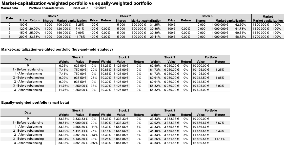
Source: simulations and calculations by the author.
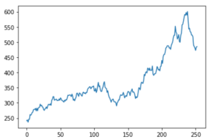
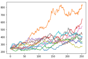
The simulation unveiled that the market-capitalization-weighted portfolio’s size anomaly failed to capture the outperformance of small-cap stocks, resulting in results that were lower than those of the smart beta equally weighted portfolio, which had a good exposure to small caps (Figure 2). The key point of this simulated model is that the market-cap indexation has a defect related to the concentration of large companies in the profile of small caps which represent a small percentage of the index. The size factor is based on a risk factor that aims to capture the documented outperformance of small-cap firms compared to larger enterprises. With this simulated model, we have proven with a very simple model in the conception that the size anomaly can indeed be a vector of return, as researched in the paper of Banz (1981) which precisely describes this concept on the US equity market (Figure 2).
Figure 2. market-capitalization-weighted portfolio vs equally-weighted portfolio.
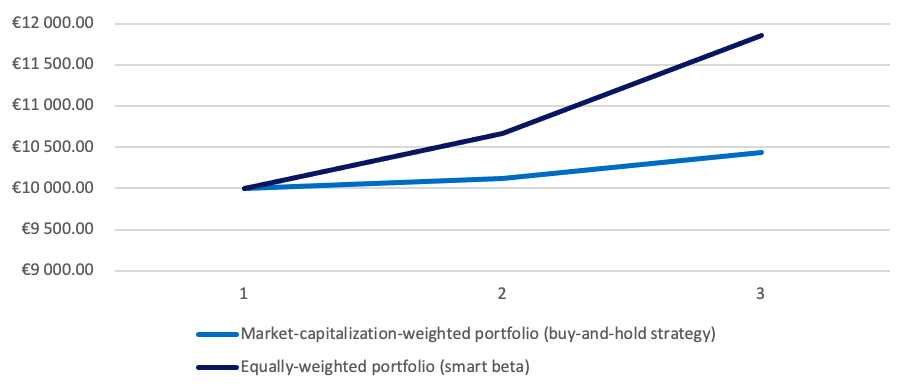
Source: simulations and calculations by the author.
One aspect to consider in this case analysis is that one of the possible explanations for this outperformance is that the weights are changed at rebalancing dates rather than allowed to drift with the price fluctuations, which is a clear distinction between cap-weighted indexes and smart beta strategies. Some claim that this rebalancing completely explains the success of smart beta strategies (Amenc et al, 2016). This allegation, however, does not hold up under investigation. An examination of buy-and-hold portfolios vs portfolios rebalanced at various frequencies reveals that whether or not rebalancing improves performance is dependent on the return behavior of the assets in the portfolio. Rebalancing may or may not provide better results than buy-and-hold tactics (Amenc et. al., 2016).
Even if beneficial rebalancing impacts occur, Smart Beta methods may not be able to capture them. Contrary to popular belief, data shows that rebalancing an equal-weighted approach more frequently does not always increase performance. Furthermore, both short- and long-term reversal effects are empirically insignificant in explaining the performance of a wide variety of Smart Beta strategies. Naturally, rebalancing is necessary, especially to maintain diversity and target factor exposures. Rebalancing, on the other hand, is not an experimentally verified source of Smart Beta strategy performance (Amenc et. al., 2016).
Smart beta: passive or active investment strategy?
Smart beta investing is considered a hybrid strategy because it attempts to replicate the performance of a predetermined benchmark without engaging in market timing or stock picking, and an active strategy because investors choose to gain exposure to specific factors (beyond the market factor) by rebalancing the portfolio according to some rules. In practice, smart beta strategies often imply rebalancing to maintain target weights for each factor. In this sense, smart beta strategies are active, or at least more active than the buy-and-hold strategy. However, the rebalancing of portfolios of smart beta strategies is usually done with a predefined rule. In this sense, smart beta strategies are passive, or at least more passive than discretionary investment strategies based on stock picking and market timing.
Why should I be interested in this post?
If you are a business school or university undergraduate or graduate student, this content will help you in understanding the various evolutions of asset management throughout the last decades and in broadening your knowledge of finance beyond the classical 101 course.
Smart beta funds have become a hot issue among investors in recent years. Smart beta is a game-changing invention (or just a new marketing idea?) that addresses an unmet need among investors: a higher return for lower risk, net of transaction and administrative costs. In a way, these tactics create a new market. As a result, smart beta is gaining traction and influencing the asset management market.
Related posts on the SimTrade blog
▶ Youssef LOURAOUI Factor Investing
▶ Youssef LOURAOUI Origin of Factor Investing
Factor series
▶ Youssef LOURAOUI Size Factor
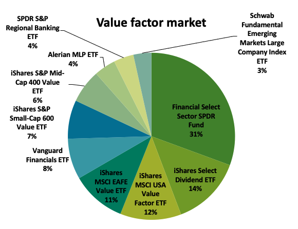
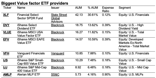
▶ Youssef LOURAOUI Value Factor
▶ Youssef LOURAOUI Yield Factor
▶ Youssef LOURAOUI Momentum Factor
▶ Youssef LOURAOUI Quality Factor
▶ Youssef LOURAOUI Growth Factor
▶ Youssef LOURAOUI Minimum Volatility Factor
Useful resources
Academic research
Amenc, N., Ducoulombier, F., Goltz, F. and Ulahel, J., 2016. Ten misconceptions about smart beta. EDHEC Risk Institute Working paper.
Banz, R.W., 1981. The relationship between return and market value of common stocks. Journal of Financial Economics, Volume 9, pp. 3-18.
Fama, E.F., French, K.R., 1992. The cross-section of expected stock returns. The Journal of Finance, 47: 427-465.
Grossman, S., Stiglitz, J., 1980. On the impossibility of Informationally efficient markets. The American Economic Review, 70(3), 393-408.
Jensen, M.C. 1968. The performance of mutual funds from 1945–1964. The Journal of Finance, 23:389-416.
Malkiel, B., 1995. Returns from Investing in Equity Mutual Funds 1971 to 1991. The Journal of Finance, 50(2):549-572.
Business analysis
BlackRock Research, 2021. What is Factor Investing?
About the author
The article was written in September 2021 by Youssef LOURAOUI (ESSEC Business School, Global Bachelor of Business Administration, 2017-2021).