Types of exercise for option contracts

Types of exercise for option contracts

Akshit Gupta

This article written by Akshit GUPTA (ESSEC Business School, Grande Ecole Program – Master in Management, 2019-2022) presents the different types of exercise for option contracts.

Introduction

Exercising a call option contract means the purchase of the underlying asset by the call buyer at the price set in the option contract (strike price). Similarly, exercising a put option contract means the sale of the underlying asset by the put buyer at the price set in the option contract.

The different option contracts can be settled in cash or with a physical delivery of the underlying asset. Normally, the equity, fixed interest security and commodity option contracts are settled using physical delivery and index options are settled in cash.

Majority of options are not exercised before the maturity date because it is not optimal for the option holder to do so. Note that for options with physical delivery, it may be better to close the position before the expiration date). If an option expires unexercised, the option holder loses any of the rights granted in the contract (indeed, in-the-money options are automatically exercised at maturity). Exercising options is a sophisticated and at times a complicated process and option holder need to take several factors into consideration while making the decision about exercise such as opinion about future market behavior of underlying asset in option, tax implications of exercise, net profit that will be acquired after deducting exercise commissions, option type, vested shares, etc.

Different types of exercise for option contracts

The option style does not deal with the geographical location of where they are traded! The contracts differ in terms of their expiration time when they can be exercised. The option contracts can be categorized as per different styles they come in. Some of the most common styles of option contracts are:

American options

American-style options give the option buyer the right to exercise his/her option anytime prior or up to the expiration date of the contract. These options provide greater flexibility to the option buyer but also come at a higher price as compared to the European-style options.

European options

European-style options can only be exercised on the expiration or maturity date of the contract. Thus, they offer less flexibility to the option buyer. However, the European options are cheaper as compared to the American options.

Bermuda options

Bermuda options are a mix of both American and European style options. These options can only be exercised on specific predetermined dates or periods up to the expiration date. They are considered to be exotic option contracts and provide limited flexibility to the option buyer.

Early Exercise

Early exercise is a strategy of exercising options before the expiration date and is possible with American options only. The question is: when the holder of an American option should exercise his/her option? Before the expiration date or at the expiration date? Quantitative models say that it could be optimal to exercise American options before the date of a dividend payout (options are not protected against the payement of dividends by firms) and sometimes for deep in-the-money put options.

There are many strategies that investors follow while exercising option contracts in order to maximize their gains and hedge risks. A few of them are discussed below:

Exercise-and-Hold

Investors can purchase their option shares with cash and hold onto them. This allows them to benefit from ownership in company stock, providing potential gains from any increase in stock value and dividend payments if any. Investors are also liable to pay brokerage commissions fees and taxes.

Exercise-and-Sell

This is a cashless strategy wherein investors purchase the option shares and then immediately sell them. Brokerages generally allow this kind of transaction without use of cash, with the money from the stock sale covering the purchase price, as well as the commissions and taxes associated with the transaction. This choice provides investors with available cash in pocket to invest elsewhere too.

Exercise-and-Sell-to-Cover

In this strategy too, investors exercise the option and then immediately sell enough shares to cover the purchase price, commissions fees and taxes. The remaining shares remain with the investor.

Related posts on the SimTrade blog

   ▶ All posts about Options

   ▶ Akshit GUPTA Options

   ▶ Akshit GUPTA Analysis of the Rogue Trader movie

   ▶ Akshit GUPTA History of Options markets

   ▶ Akshit GUPTA Option Trader – Job description

Useful Resources

Academic research

Hull J.C. (2015) Options, Futures, and Other Derivatives, Ninth Edition, Chapter 10 – Mechanics of options markets, 235-240.

Business analysis

Fidelity Exercising Stock Options

About the author

Article written in August 2021 by Akshit GUPTA (ESSEC Business School, Grande Ecole Program – Master in Management, 2019-2022).

Mon expérience lors de la fusion Lafarge Holcim

Mon expérience lors de la fusion Lafarge Holcim

Oliver Begue.jpg

In this article, Oliver BEGUE (ESSEC Executive Education, Mastère Spécialisé Direction Financière Contrôle, 2020-2021) nous partage son expérience professionnelle lors de la fusion d’entreprises Lafarge Holcim en avril 2014.

La fusion Lafarge Holcim

Lafarge

En 2015 Lafarge était une entreprise française devenue numéro 1 mondial dans la production de ciment, béton et granulats dans le secteur du BTP avec un chiffre d’affaires de 12,8 Mds d’euros. Lafarge était côté à Euronext et faisait partie de l’indice CAC 40 avec une capitalisation boursière de 16,7 Mds d’euros.

Holcim

En 2015 Holcim est une entreprise suisse devenue numéro 2 mondial du même secteur d’activité que Lafarge (BTP) avec un chiffre d’affaires converti en euros de 19,9 Mds d’euros. Holcim était coté à la Bourse suisse (Swiss EBS Stocks) avec une capitalisation boursière convertie en euro de 21,5 Mds d’euros.

L’opération de fusion des deux entreprises

Le 5 septembre 2015, les deux groupes, Lafarges et Holcim, ont annoncé leur projet de fusion d’égal à égal (1 action Holcim pour 1 action Lafarge). Cette fusion avait deux principaux objectifs :

  • Générer de la trésorerie pour les actionnaires (dividendes par de meilleurs résultats)
  • Devenir le géant mondial du BTP pour concurrencer les entreprises fabriquant à bas couts des pays émergents.

Bilan de la fusion

L’opération de fusion a coûté plus de 2 Mds d’euros au Groupe soit le double du budget prévu. La Commission européenne, afin de valider la fusion des deux géants du BTP, a demandé la cession d’un périmètre de sociétés rentables des deux Groupes afin de maintenir la politique de concurrence de l’Union Européenne.

La fusion elle-même, et le volume d’entités cédées ont ainsi fait la une des journaux en 2015 et 2016 soulevant nombre de scandales (financement du terrorisme, obtention de l’appel d’offre du mur entre le Mexique et les Etats-Unis, présence non officielle en Iran…)
Depuis la fusion et suite à ces différents évènements, le Groupe a connu un désengagement de ses clients ayant pour conséquence la chute de son chiffre d’affaires qui atteint en 2019 24,6 Mds d’euros avec une capitalisation boursière de 27,2 Mds d’euros.

Le Groupe LafargeHolcim, en crise de croissance, rattrapé par la concurrence et les nouveaux marchés plus porteurs, et subissant le désintérêt sur le marché (chute du volume d’échanges) quitte ainsi le CAC 40 en juin 2018.

Mon expérience personnelle

La fusion Lafarge Holcim est un réel succès dans ma carrière professionnelle. En plus du volume de données à traiter étant donné la taille du groupe, les spécificités de chacun (groupe français intégré par un groupe suisse-allemand, deux outils de consolidation différents, un traitement normatif et une communication différence, une gestion RH différente), le réel challenge chez Lafarge Holcim était pour moi une question de légitimité. A à peine 24 ans, j’étais amené à valider des transactions, mais surtout à former des équipes (des centaines de personnes) aux nouveaux outils de consolidation. Former des équipes ayant mon âge en nombre d’année d’expérience fut compliqué. J’ai dû prouver mes compétences techniques et faire preuve d’empathie dans un contexte humain difficile afin de gagner la confiance de mes interlocuteurs.

Cette fusion a bel et bien été un tremplin dans ma carrière professionnelle. Néanmoins, je doute qu’elle ait été positive pour le Groupe.

Fusion d’entreprises : création de valeur ?

La fusion d’entreprises présentent des avantage set des inconvénients que nous listons ci-dessous :

Avantage :

A cout terme, la fusion Lafarge Holcim a bénéfié d’une réduction des couts fixes liés aux synergies (fermeture totale du siège social de Lafarge notamment), pour un total de 1,4 Mds d’euros. La fusion de ces deux Groupes permet aussi, dans un secteur où les ressources employées en investissements sont particulièrement important, à mutualiser les ressources et le réseau géographique en termes de périmètre de société du nouveau Groupe. Ainsi Le groupe accroîtrait sa solidité financière avec une forte génération de cash-flow et un bilan robuste.

Les implantations des deux entreprises sont complémentaires, Lafarge apportant une forte présence en Afrique et au Moyen-Orient ; Holcim, des positions majeures en Amérique latine et en Asie pacifique. La réunion de ces deux portefeuilles permettra au nouveau Groupe de disposer d’une présence géographique équilibrée dans 90 pays, dont 73 pays émergents.

Inconvénients :

Afin d’obtenir la validation de la Commission Européenne sur la fusion, les deux Groupes se sont accordés pour procéder à la cession d’un parc important d’actifs, principalement des filiales en croissance pour un total d’environ 6,5 Mds d’euros.

Aussi les synergies espérées ne représentent au total que 3,5% de la capitalisation du nouvel ensemble, ce qui est peu et ne sera pas suffisant pour combler les pertes liées au Chiffre d’affaires (scandales) et au besoin en financement toujours grandissant.

L’objectif de la fusion était de créer un géant du BTP leader incontesté du marché. Le résultat est un Groupe de taille moyenne, déficitaire, et qui tente de se désendetter en cédant toujours plus de filiales.

Articles similaires sur le blog SimTrade

   ▶ All posts about Professional experiences

   ▶ Louis DETALLE The abandonment of the TF1-M6 fusion: what happened?

   ▶ Basma ISSADIK My experience as an M&A Analyst Intern at Oaklins Atlas Capital

Ressources utiles

Rapport annuel 2014 de Lafarge

Rapport annuel 2015 de Lafarge Holcim

La Commission autorise l’acquisition, sous conditions, de Lafarge par Holcim

Précisions de Lafarge Holcim sur ses opérations en Syrie

A propos de l’auteur

Cet article a été écrit en septembre 2021 par Oliver BEGUE (ESSEC Executive Education, Mastère Spécialisé Direction Financière Contrôle, 2020-2021).

VIX index

VIX index

Youssef_Louraoui

In this article, Youssef LOURAOUI (ESSEC Business School, Global Bachelor of Business Administration, 2017-2021) presents the VIX index, which is a financial index that measures the uncertainty in the US equity market.

This article is structured as follows: we begin by defining the grounding notions of the VIX index. We then explain the behavior of this index and its statistical characteristics. We finish by presenting its practical usage in financial markets.

Definition

The CBOE Volatility Index, abbreviated “VIX”, is a measure of the expected S&P 500 index movement calculated by the Chicago Board Options Exchange (CBOE) from the current trading prices of options written on the S&P 500 index.

Known as Wall Street’s “fear index”, the VIX is closely monitored by a broad range of market players, and its level and pattern have become ingrained in market discussion.

Figure 1 illustrates the evolution of the VIX index for the period from 2003 to 2021.
Figure 1 Historical levels of the VIX index from 2003-2021.
VIX_levels_analysis
Source: computation by the author (Data source: Thomson Reuters).

VIX values greater than 20 are regarded to be high by market participants. If the VIX is between 12 and 20, it is considered normal; if it is less than 12, it is considered low. As it is the case with other indices, the VIX is computed using the price of a basket of tradable components (in this case, options expiring within the next month or so). The profit or loss that option buyers and sellers realize during the option’s life will depend, among other things, on how significantly the S&P 500’s actual volatility will differ from the implied volatility given by the VIX at the start of the period (S&P Global Research, 2017).

Behavior of the VIX index

Statistical distribution of the S&P500 index returns and VIX level

Figure 2 displays the statistical distribution of the price variations in the S&P500 index for different levels of the VIX index The higher the VIX index (by convention, greater than 20), the more severe the distribution tends to be, with negative skewness and high kurtosis indicating heightened volatility in the US market, therefore exacerbating both positive and negative swings. An opposite finding may be made for the VIX level at lower levels (often less than 12), when market swings are less evident due to less skewness and lower kurtosis (S&P Global Research, 2017).

Figure 2. The distribution of 30-day return in the S&P500 index for different VIX index levels.
Statistical distribution of the S&P500 index returns
Source: S&P Global Research (2017).

If the VIX is low, market players may benefit by purchasing options; conversely, if the VIX is high, market participants may profit from selling options. The specific utility of anticipated VIX is that it gives us with a more accurate assessment of whether VIX is high, low, or normal at any point in time (S&P Global Research, 2017). Thus, VIX may be regarded of as a crowd-sourced estimate of the S&P 500’s expected volatility. As with interest rates and dividends, one cannot invest directly in them, even though one can guess on their future worth, one cannot invest directly in VIX, and the significance of a specific VIX level is commonly misinterpreted (S&P Global Research, 2017).

Recent volatility in the S&P500 index and VIX level

Figure 3 demonstrates that the VIX index is strongly correlated with recent market volatility. However, there is considerable variance; for example, a recent volatility level of about 20% has been associated with a VIX level of 34 (point B, when VIX was very “high”) and with a VIX level of 12 (point C, when VIX was relatively “low”). Volatility (realized or implied) has a strong propensity to return to its mean. This insight is not especially original, despite its illustrious past. There is an enormous body of data demonstrating that volatility tends to mean revert across markets, and the pioneers of this field were given the Nobel Prize in part for incorporating their results into volatility forecasts and simulations (S&P Global Research, 2017).

Figure 3. Relation between VIX and recent volatility.
VIX_regression_analysis
Source: S&P Global Research (2017).

Realized volatility in the S&P500 index and VIX level

Figure 4 represents the relationship between Realized volatility in the S&P500 index over a period and the VIX level at the begining of the period.

Figure 4. VIX versus next realized volatility.
VIX_realized_graph
Source: S&P Global Research (2017).

Mean reversion

Figure 5 shows how VIX index converge to a certain llong-term level as time passes. This finding is not due to 15% being exceptional in any manner; this figure for M was calculated using historical volatility levels for the S&P 500 and their evolution. It is not implausible that M (else referred to as long-term average volatility in the US equities market) may change over time; changes in the S&P 500’s sector weightings, trade All of these factors have the ability to influence both the pace and the volume and the point at which mean reversion occurs.

Figure 5. Mean-reversion dynamic in recent volatility.
VIX mean reversion
Source: S&P Global Research (2017).

Use of the VIX index in financial markets

There are two methods for determining an asset’s volatility. Either through a statistical calculation of an asset’s realized volatility, also known as historical volatility, which serves as a pointer to the asset’s volatility behavior. This is a limited method that is based on the premise that past volatility tends to replicate itself in the future, without including a forward-looking study of volatility. The second technique is to extract an asset’s volatility from option prices referred to as “implied volatility”.

Why should I be interested in this post?

When investors make investment decisions, they utilize the VIX to gauge the degree of risk, worry, or stress in the market. Additionally, traders can trade the VIX using a range of options and exchange-traded products, or price derivatives using VIX values.

Related posts on the SimTrade blog

   ▶ All posts about Options

   ▶ Akshit GUPTA Options

   ▶ Akshit GUPTA History of Option Markets

   ▶ Jayati WALIA Implied Volatility

   ▶ Youssef LOURAOUI Minimum Volatility Factor

Useful resources

Business analysis

CBOE , 2021. VIX

Nasdaq, 2021. Realized Volatility

Nasdaq, 2021. Vix Index Volatility

S&P Global Research, 2017. Reading VIX: Does VIX Predict Future Volatility?

S&P Global Research, 2017. A Practitioner’s Guide to Reading VIX

About the author

The article was written in September 2021 by Youssef LOURAOUI (ESSEC Business School, Global Bachelor of Business Administration, 2017-2021).

Factor Investing

Factor Investing

Youssef_Louraoui

In this article, Youssef LOURAOUI (ESSEC Business School, Global Bachelor of Business Administration, 2017-2021) presents factor investing, which is an investment approach that focuses on distinct performance drivers across asset classes.

This article is structured as follows: we begin with the early works of factor investing (market factor). We then delve more in detail on the different factors available and their characteristics. We finish with an empirical analysis that aims to capture the performance of factor investing across time.

Early works

In the world of investing, a factor is a persistent driver that helps explain assets’ long-term risk and return properties across asset classes. It is important to understand how factors work to better capture their potential for excess return and reduced risk across asset classes.

As a result of Harry Markowitz’s prior studies, William Sharpe, John Lintner, and Jan Mossin independently developed the Capital Asset Pricing Model (CAPM). The CAPM was a significant evolutionary step forward in capital market equilibrium theory because it allowed investors to value assets correctly in terms of systematic risk that impact all assets (Mangram, 2013). In the CAPM, the factor is the market factor representing the global uncertainty of the market.

In the late 1970s, the portfolio management industry aimed to capture the market portfolio return, but as financial research advanced and certain significant contributions were made, this gave rise to other factor characteristics to capture some additional performance.

Factor investing

As defined by Blackrock (2021), “Factor investing” is an investment strategy that focuses on unique determinants of performance across asset classes. Factor investing may improve portfolio performance and decrease volatility by increasing portfolio diversification. Asset returns are driven by two main types of factors: macroeconomic factors and style factors. Macroeconomic factors capture broad risks across asset classes while style factors explain returns and risk within asset classes.

Considering macroeconomic factors, returns can be influenced by the following macroeconomic variables (BlackRock research, 2021):

  • Economic growth: exposure to business and market cycles
  • Real interest rates: sensitivity to interest rate movements
  • Inflation: exposure to change in price
  • Credit: default risk from lending to companies
  • Emerging markets: political and sovereign risk
  • Liquidity: holding liquid assets.

Considering style factors, returns can be influenced by the following style variables (BlackRock research, 2021):

  • Value: stocks discounted to relative value
  • Minimum volatility: stable, lower risk stocks
  • Momentum: stocks with upward price trends
  • Quality: financially healthy companies
  • Size: smaller, high growth companies
  • Growth: companies that have a rate of growth above the market growth
  • Yield: companies that have undervalued and stable dividends

Characteristics of a factor

As defined in the work of Ang (2013) a factor must comply with the following characteristics:

  • A factor must be backed up by scholarly research: factors should have an academic basis. The research should illustrate either compelling logical reasoning or compelling behavioral biases, or both, in order to adequately justify the risk premium (Ang, 2013). Value, momentum, and minimum volatility among other strategies qualify as adequate risk factors under this criterion. New research may find new factors, qualify prior agreement on recognized factors, or even reject factors previously identified, all of which may be used to shape investment strategy.
  • A factor must have maintained a substantial risk premium in the past and is anticipated to do so in the future: not only should investors understand why the risk premium existed in the past, but they should also have some reason to believe that it will continue to exist in the future (at least in the short run). By definition, factors are systematic–they emerge from risk or behavioral patterns that will likely continue (again, in the short run), even if everyone is aware of the factors and many investors pursue the same factor strategies (no crowding effect).
  • A factor must be capable of being implemented in liquid, tradable instruments: factor strategies should be very inexpensive, which is best done via the use of liquid securities.

Academic literature on factor investing

Numerous academic studies and years of investing experience have revealed some types of stock, debt, and derivative assets with larger payoffs than the broad market index. Over extended periods of time, equities with low price-to-book ratios (value stocks) outperform those with high price-to-book ratios (growth stocks), creating a value-growth premium (Ang, 2013). Over time, equities with a history of high or positive returns (winners) outperform those with a history of low or negative returns (losers). This is at the heart of momentum strategies, which seeks to get exposure to stocks that have a winning tendency in the upside and downside assuming that they will continue to do well in the short term (Ang, 2013).

Investors seeking downside protection in a turbulent market environment may increase exposure to low volatility strategies, while those comfortable with more risk may choose for higher-return strategies such as momentum. The financial literature has explored deeper to show that some factors have had a long-term impact on returns. These factors contributed to returns for three reasons: an investor’s desire to take on risk, structural obstacles, and the reality that not all investors are not always entirely rational (BlackRock research, 2021). Particular factors yield higher returns as a result of increased risk but may underperform in certain market conditions. Enhanced methods use factors in more sophisticated ways, such as trading across various asset classes and sometimes investing in both long and short positions. These improved factor strategies are used by investors seeking absolute returns or as a supplement to hedge funds and classic active strategies (BlackRock research, 2021).

Securities that are less liquid trade at a discount to their more liquid counterparts and earn a higher average excess return on average. As a result, a premium is charged for illiquidity (Ang, 2013). Bonds with a greater risk of default often have higher average returns, owing to the credit risk premium. Additionally, because investors are ready to pay for protection against periods of extreme volatility, when returns tend to fall, sellers of volatility protection in option markets receive a high rate of return on average (Ang, 2013). As a result, investors can collect the premiums as follows (Ang, 2013):

  • The value-growth premium is equal to the difference between value and growth stocks.
  • The momentum premium is equal to the difference between winning and losing stocks.
  • The illiquidity premium is equal to the difference between the value of illiquid assets and the value of liquid assets.
  • The credit risk premium is the difference between the return on risky and safe debt.

These are dynamic factors, since they reflect time-varying holdings in securities that fluctuate in value over time. While dynamic factors frequently outperform the market over extended periods of time, they can significantly underperform at select occasions — such as the 2008-2009 financial crisis. While dynamic factors frequently outperform the market over extended periods of time, they can outperform the market significantly at select moments — such as the 2008-2009 financial crisis. In the long term, factor risk premiums exist to compensate investors for experiencing losses during difficult times (Ang, 2013). In the end, the factors are not ideal for everyone due to the inherent risk associated with factor techniques.

Empirical analysis

Hodges et al. (2017) published a study in the Journal of Portfolio Management that looks at the performance of factor funds over a 30-year period and examines the vectors of returns). Figure 1 illustrates the average excess returns (above the MSCI USA Index) of each factor from June 30, 1988 to September 30, 2016. Value, quality, momentum, and size all have positive average returns; momentum and value have the largest annual excess returns of 3.4 percent and 1.5 percent, respectively. Minimum volatility has generated an average return comparable to the market (but with less risk), similar with Ang’s findings (Hodges et al., 2017).

Figure 1. Factor analysis from 1988 – 2016. Average excess return.

Average_excess_return_Smart_Beta_JPM_AM
Source: Hodges et al. (2017).

Figure 2 plots 12-month moving averages of excess factor returns and demonstrates that, while long­run excess premiums are positive, there is significant temporal variation throughout the sample. For instance, size changes from a negative 12-month mean return of -2.0 percent in 1999 to a positive 12-month mean return of 3.0 percent in the early 2000s.

Figure 2. Smart beta excess returns for the period from 1988 to 2016.

Excess_return_Smart_Beta_JPM_AM
Source: Hodges et al. (2017).

Figure 3 demonstrates that the excess factor returns are not substantially correlated: the lowest correlation is -0.42, while the largest is 0.67, between minimal volatility and size. Notably, momentum and value are negatively connected with a correlation coefficient of -0.22, which is consistent with their well-known negative association (Hodges, et al., 2017).

Figure 3. Correlation analysis of smart beta excess returns for the period from 1988 to 2016.

Correlation_analysis_Smart_Beta_JPM_AM
Source: Hodges et al. (2017).

Why should I be interested in this post?

Numerous equity investors seeking greater returns at a cheaper cost have shifted their focus to factor investing. Active managers in the traditional sense typically make investing decisions based on their research of particular companies and their stocks. By contrast, factor strategies identify the qualities, or factors, that are most likely to beat the market and then invest in stocks that exhibit those characteristics. For instance, the value factor is based on the strategy of investing in companies that are undervalued in comparison to the market, whereas the momentum factor is based in the strategy of investing in equities that have recently seen a price acceleration.

Related posts on the SimTrade blog

   ▶ Youssef LOURAOUI Size Factor

   ▶ Youssef LOURAOUI Value Factor

   ▶ Youssef LOURAOUI Yield Factor

   ▶ Youssef LOURAOUI Momentum Factor

   ▶ Youssef LOURAOUI Quality Factor

   ▶ Youssef LOURAOUI Growth Factor

   ▶ Youssef LOURAOUI Minimum Volatility Factor

Useful resources

Academic research

Ang, A., 2013. Factor Investing. Working paper.

Hodges, P., Hogan, K., Peterson, J. R., Ang, A., 2017. Factor Timing with Cross- Sectional and Time-Series Predictors. The Journal of Portfolio Management 44(1): 30-43.

Business Analysis

BlackRock research, 2021. What is Factor Investing?

About the author

The article was written in September 2021 by Youssef LOURAOUI (ESSEC Business School, Global Bachelor of Business Administration, 2017-2021).

Origin of factor investing

Origin of factor investing

Youssef_Louraoui

In this article, Youssef LOURAOUI (ESSEC Business School, Global Bachelor of Business Administration, 2017-2021) presents the origin of factor investing. A factor is defined as a persistent driver that helps explain assets’ long-term risk and return properties across asset classes.

This article is structured as follows: we begin by presenting Markowitz’s Modern Portfolio Theory (MPT) as the origin of factor investing (market factor). We then explain the Fama-French three-factor models, which is an extension of the CAPM single factor model (market factor). Furthermore, we explain also the Carhart four-factor model and the Fama-French five-factor model that aimed to capture additional factors to the market factor.

Markowitz’s Modern Portfolio Theory: Origin of the factor investing

Factor investing can be retraced to the work of Harry Markowitz in the early 1950s. The most important aspect of Markowitz’s approach was his fundamental finding that an asset’s risk and return should not be evaluated on its own, but rather on how it contributes to the entire risk and return of a portfolio. His dissertation, titled “Portfolio Selection”, was published in The Journal of Finance (1952). Nearly thirty years later, Markowitz shared the Nobel Prize for economics and corporate finance for his MPT contributions to both disciplines. The holy grail of Markowitz’s work is based on his calculation of the variance of a two-asset portfolio computed as follows:

Markowitz_2_asset_MV

Where:

  • w and (1-w) represents asset weights of assets A and B
  • σ2 represents the variance of the assets and portfolio
  • cov(rA,rB) represents the covariance of assets A and B.

Capital Asset Pricing Model (CAPM)

William Sharpe, John Lintner, and Jan Mossin separately developed another key capital markets theory as a result of Markowitz’s previous works : the Capital Asset Pricing Model (CAPM). The CAPM was a huge evolutionary step forward in capital market equilibrium theory, since it enabled investors to appropriately value assets in terms of systematic risk, defined as the market risk which cannot be neutralized by the effect of diversification. In his derivation of the CAPM, Sharpe, Mossin and Litner made significant contributions to the concepts of the Efficient Frontier and Capital Market Line. Sharpe, Litner and Mossin seminal contributions would later earn him the Nobel Prize in Economics. The CAPM is based on a set of market structure and investor hypotheses:

  • There are no intermediaries
  • There are no limits (short selling is possible)
  • Supply and demand are in balance
  • There are no transaction costs
  • An investor’s portfolio value is maximized by maximizing the mean associated with projected returns while reducing risk variance
  • Investors have simultaneous access to information in order to implement their investment plans
  • Investors are seen as “rational” and “risk averse”.

Under this framework, the expected return of a given asset is related to its risk measured by the beta:

CAPM

Where :

  • E(r) represents the expected return of the asset
  • rf the risk-free rate
  • β a measure of the risk of the asset
  • E(rm) the expected return of the market
  • E[rm– rf]represents the market risk premium.

In this model, the beta (β) parameter is a key parameter and is defined as:

Beta

Where:

  • Cov(r, rm) represents the covariance of the asset with the market
  • σ2(rm) is the variance of market return.

The beta is a measure of how sensitive an asset is to market swings. This risk indicator aids investors in predicting the fluctuations of their asset in relation to the wider market. It compares the volatility of an asset to the systematic risk that exists in the market. The beta is a statistical term that denotes the slope of a line formed by a regression of data points comparing stock returns to market returns. It aids investors in understanding how the asset moves in relation to the market. According to Fama and French (2004), there are two ways to interpret the beta employed in the CAPM:

  • According to the CAPM formula, beta may be thought in mathematical terms as the slope of the regression between the asset return and the market return. Thus, beta quantifies the asset sensitivity to changes in the market return;
  • According to the beta formula, it may be understood as the risk that each dollar invested in an asset adds to the market portfolio. This is an economic explanation based on the observation that the market portfolio’s risk (measured by 〖σ(r_m)〗^2) is a weighted average of the covariance risks associated with the assets in the market portfolio, making beta a measure of the covariance risk associated with an asset in comparison to the variance of the market return.

Additionally, the CAPM makes a distinction between two forms of risk: systematic and specific risk. Systematic risk refers to the risk posed by the market’s basic structure, its participants, and any and all non-diversifiable elements such as monetary policy, political events, and natural disasters. By contrast, specific risk refers to the risk inherent in a particular asset and so is diversifiable. As a result, the CAPM solely captures systematic risk via the beta measure, with the market’s beta equal to one, lower-risk assets having a beta less than one, and higher-risk assets having a beta larger than one.

Finally, the CAPM’s central message is that when investors invest in a particular security/portfolio, they are rewarded twice: once via the time value of money impact (reflected in the risk-free component of the CAPM equation) and once via the effect of taking on more risk. However, the CAPM is not an empirically sound model, owing to an unnecessarily simplified set of assumptions and problems in establishing validating tests at the model’s first introduction (Fama and French, 2004). Thus, throughout time, the CAPM has been revised and modified to address not just its inadequacies but also to keep pace with financial and economic changes. Sharpe (1990), in his evaluation of the CAPM, cites various examples of revisions to his basic model proposed by other economists and financial experts.

The Fama-French three-factor model

Eugene Fama and Kenneth French created the Fama-French Three-Factor model in 1993 in response to the CAPM’s inadequacy. It contends that, in addition to the market risk component introduced by the CAPM, two more factors affect the returns on securities and portfolios: market capitalization (referred to as the “size” factor) and the book-to-market ratio (referred to as the “value” factor). According to Fama and French, the primary rationale for include these characteristics is because both size and book-to-market (BtM) ratios are related to the economic fundamentals of the business issuing the securities (Fama and French, 1993).

They continue by stating that:

  • Earnings and book-to-market ratios are inversely associated, with companies with low book-to-market ratios consistently reporting better earnings than those with high book-to-market ratios
  • Due to a similar risk component, size and average returns are inversely associated. This is based on their observation of the trajectory of small business profits in the 1980s: they suggest that small enterprises experience longer durations of earnings depression than larger enterprises in the event of a recession in the economy in which they operate. Additionally, they noted that smaller enterprises did not contribute to the economic expansion in the mid- and late-1980s following the 1982 recession
  • Profitability is connected to both size and BtM, and is a common risk factor that emphasizes and explains the positive association between BtM ratios and average returns. As thus, the return on a security/portfolio becomes:

FF_3FM

Where :

  • E(𝑟) is the expected return of the asset/portfolio
  • 𝑟𝑓 is the risk-free rate
  • 𝛽 is the measure of the market risk of the asset
  • 𝐸(𝑟𝑀) is the expected return of the market
  • 𝛽𝑆 is the measure of the risk related to the size of the asset
  • 𝛽𝑉 is the measure of the risk related to the value of the security/portfolio
  • 𝑆𝑀𝐵 (which stands for “Small Minus Big”) measures the difference in expected returns between small and big firms (in terms of market capitalization)
  • 𝐻𝑀𝐿 (which stands for “High Minus Low”) measures the difference in expected returns between value stocks and growth stock
  • 𝛼 is a regression intercept
  • 𝜖 is a measure of regression error

Both SMB and HML are derived using historical data as well as a mixture of portfolios focused on size and value. Professor French publishes these values on a regular basis on his personal website. Meanwhile, the betas for both the size and value components are derived using linear regression and might be positive or negative. However, the Fama-French three-factor model is not without flaws. Griffin (2002) highlights a significant flaw in the model when he claims that the Fama-French components of value and size are more accurate at explaining return differences when applied locally rather than internationally. As a result, each of the components should be addressed on a nation-by-country basis (as professor French now does on his website, where he specifies the SMB and HML factors for each nation, such as the United Kingdom, France, and so on). While the Fama-French model has gone further than the CAPM in terms of breaking down security returns, it remains an incomplete model with spatially confined interpretation of its additional variables. Efforts have been made over the years to complete this model, with Fama and French adding two more variables in 2015, profitability and investment strategy, and other scholars, like as Carhart (1997), adding a fourth feature, momentum, to the original Three-Factor model.

The Carhart four-factor model

Carhart (1997) extended the Fama-French three-factor model (1993) by adding a fourth factor: momentum. Momentum is defined as the observable tendency for prices to continue climbing or declining following an initial increase or decline. By definition, momentum is an anomaly, as the Efficient Market Hypothesis (EMH) states that there is no reason for security prices to continue growing or declining after an initial change in their value.

While traditional financial theory is unable to define precisely what causes momentum in certain securities, behavioural finance provides some insight into why momentum exists; indeed, Chan, Jegadeesh and Lakonishok (1996) argue that momentum arises from the inability of the majority of investors to react quickly and immediately to new market information and, thus, integrate that information into securities. This argument demonstrates investors’ irrationality when it comes to appraising the value of certain stocks and making investing decisions. Carhart was motivated to incorporate the momentum component into the Fama-French three-factor model since the model was unable to account for return variance in momentum-sorted portfolios (Fama and French, 1996 – Carhart 1997). Carhart incorporated Jegadeesh and Titman’s (1993) one-year momentum variation into his model as a result.

Carhart_4FM

Where the additional component represents:

  • 𝛽𝑀 is the measure of the risk related to the momentum factor of the security/portfolio
  • 𝑈𝑀𝐷 (which stands for “Up Minus Down”) measures the difference in expected returns between “winning” securities and “losing” securities (in terms of momentum).

As Carhart states in his article, the four-factor model, like the CAPM and the Fama-French Three-Factor, may be used to explain the sources of return on a specific security/portfolio (Carhart, 1997).

The Fama-French five-factor model

Fama and French state in 2014 that the first three-factor model they developed in 1993 does not adequately account for certain observed inconsistencies in predicted returns. As a consequence, Fama and French enhanced the three-factor model by adding two new variables: profitability and investment. The justification for these two factors arises from the theoretical implications of the dividend discount model (DDM), which claims that profitability and investment help to explain the returns achieved from the HML element in the first model (Fama and French, 2015).

Surprisingly, unlike the Carhart model, the new Fama-French model does not incorporate the momentum element. This is mostly because to Fama’s position on momentum. While not denying its existence, Fama thinks that the degree of risk borne by securities in an efficient market cannot fluctuate so dramatically that it justifies the necessity to recognize the momentum factor’s involvement (Fama and French, 2015). According to the Fama-French five-factor model, the return on any security is calculated as follows:

FF_5F

  • 𝛽P is the measure of the risk related to the profitability factor of the security/portfolio
  • 𝑅𝑀𝑊 (which stands for “Robust Minus Weak”) measures the difference in expected returns between securities that exhibit strong profitability levels (thus making them “robust”) and securities that show inconsistent profitability levels (thus making them “weak”)
  • 𝛽𝐼 is the measure of the risk related to the investment factor of the asset
  • 𝐶𝑀𝐴 (which stands for “Conservative Minus Aggressive”) measures the difference in expected returns between securities that engage in limited investment activities (thus making them “conservative”) and securities that show high levels of investment activity (thus making them “aggressive”).

To validate the new model, Fama and French created many portfolios with considerable returns disparities due to size, value, profitability, and investing characteristics. Additionally, they completed two exercises:

  • The first is a regression of portfolio results versus the improved model. This was done to determine the extent to which it explains the observed returns disparities between the selected portfolios
  • The second is to compare the new model’s performance to that of the three-factor model. This was done to determine if the new five-factor model adequately accounts for the observed returns differences in the old three-factor model. The following summarizes Fama and French’s conclusions about the new model.

The HML component becomes superfluous in terms of structure, since any value contribution to a security’s return can already be accounted by market, size, investment, and profitability factors. Thus, Fama and French advise investors and scholars to disregard the HML effect if their primary objective is to explain extraordinary returns (Fama and French, 2015).

They do, however, argue for the inclusion of all five elements when attempting to explain portfolio returns that display size, value, profitability, and investment tilts. Additionally, the model explains between 69% and 93% of the return disparities seen following the usage of the prior three-factor model (Fama and French, 2015). This new model, however, is not without flaws. Blitz, Hanauer, Vidojevic, and van Vliet (henceforth referred to as BHVV) identified five problems with the new Fama-French five-factor model in their 2016 paper “Five difficulties with the Five-Factor model”.

While two of these issues are related to some of the original Fama-French three factor model’s original factors (most notably the continued existence within the model of the CAPM relationship between market risk and return, as well as the new model’s overall acceptance by the academic community while some of the original factors are still contested), several of the other issues are related to other factors. These concerns include the following (Fama and French, 2015) :

  • The lack of motion
  • The new factors introduced lack robustness. The questions here include historical (i.e., will these factors apply to data points before to 1963) and if these aspects also apply to other asset types
  • The absence of adequate empirical support for the implementation of these Fama and French components

Use of the asset pricing models

All the models presented above are mostly employed in asset management to analyze the performance of an actively managed portfolio and the overall performance of a mutual fund.

Why should I be interested in this post?

In the CAPM, the factor is the market factor representing the global uncertainty of the market. In the late 1970s, the portfolio management industry aimed to capture the market portfolio return, but as financial research advanced and certain significant contributions were made, this gave rise to other factor characteristics to capture some additional performance. Analyzing the historical contributions that underpins factor investing is fundamental in order to have a better understanding of the subject.

Useful resources

Academic research

Blitz, D., Hanauer M.X., Vidojevic M., van Vliet, P., 2018. Five Concerns with the Five-Factor Model, The Journal of Portfolio Management, 44(4): 71-78.

Carhart, M.M. (1997), On Persistence in Mutual Fund Performance. The Journal of Finance, 52: 57-82.

Fama, E.F., French, K.R., 1992. The Cross-Section of Expected Stock Returns. The Journal of Finance, 47: 427-465.

Fama, E.F., French, K.R., 2004. The Capital Asset Pricing Model: Theory and Evidence. Journal of Economic Perspectives, 18(3): 25-46.

Fama, E.F., French, K.R., 2015. A five-factor asset pricing model. Journal of Financial Economics, 116(1): 1-22.

Lintner, J. 1965a. The Valuation of Risk Assets and the Selection of Risky Investments in Stock Portfolios and Capital Budgets. The Review of Economics and Statistics 47(1): 13-37.

Lintner, J. 1965b. Security Prices, Risk and Maximal Gains from Diversification. The Journal of Finance 20(4): 587-615.

Mangram, M.E., 2013. A simplified perspective of the Markowitz Portfolio Theory. Global Journal of Business Research, 7(1): 59-70.

Markowitz, H., 1952. Portfolio Selection. The Journal of Finance, 7(1): 77-91.

Mossin, J. 1966. Equilibrium in a Capital Asset Market. Econometrica 34(4): 768-783.

Sharpe, W.F. 1963. A Simplified Model for Portfolio Analysis. Management Science 9(2): 277-293.

Sharpe, W.F. 1964. Capital Asset Prices: A theory of Market Equilibrium under Conditions of Risk. The Journal of Finance 19(3): 425-442.

Related posts on the SimTrade blog

Factor investing

   ▶ Youssef LOURAOUI Factor Investing

   ▶ Youssef LOURAOUI Is smart beta really smart?

Factors

   ▶ Youssef LOURAOUI Size Factor

   ▶ Youssef LOURAOUI Value Factor

   ▶ LYoussef LOURAOUI Yield Factor

   ▶ Youssef LOURAOUI Momentum Factor

   ▶ Youssef LOURAOUI Quality Factor

   ▶ Youssef LOURAOUI Growth Factor

   ▶ Youssef LOURAOUI Minimum Volatility Factor

About the author

The article was written in September 2021 by Youssef LOURAOUI (ESSEC Business School, Global Bachelor of Business Administration, 2017-2021).

Capital Asset Pricing Model (CAPM)

Capital Asset Pricing Model (CAPM)

Jayati WALIA

In this article, Jayati WALIA (ESSEC Business School, Grande Ecole Program – Master in Management, 2019-2022) presents the Capital Asset Pricing Model (CAPM).

Introduction

The Capital Asset Pricing Model (CAPM) is a widely used metrics for the financial analysis of the performance of stocks. It shows the relationship between the expected return and the systematic risk of investing in an asset. The idea behind the model is that the higher the risk in an investment in securities, the higher the returns an investor should expect on his/her investments.

The Capital Asset Pricing Model was developed by financial economists William Sharpe, John Lintner, Jack Treynor and Jan Mossin independently in the 1960s. The CAPM is essentially built on the concepts of the Modern Portfolio Theory (MPT), especially the mean-variance analysis model by Harry Markowitz (1952).

CAPM is very often used in the finance industry to calculate the cost of equity or expected returns from a security which is essentially the discount rate. It is an important tool to compute the Weighted Average Cost of Capital (WACC). The discount rate is then used to ascertain the Present Value (PV) and Net Present Value (NPV) of any business or financial investment.

CAPM formula

The main result of the CAPM is a simple mathematical formula that links the expected return of an asset to its risk measured by the beta of the asset:

CAPM risk beta relation

Where:

  • E(ri) represents the expected return of asset i
  • rf the risk-free rate
  • βi the measure of the risk of asset i
  • E(rm) the expected return of the market
  • E(rm)- rf the market risk premium.

The risk premium for asset i is equal to βi(E(rm)- rf), that is the beta of asset i, βi, multiplied by the risk premium for the market, E(rm)- rf.

The formula shows that investors demand a return higher than the risk-free rate for taking higher risk. The equity risk premium is the component that reflects the excess return investors require on their investment.

Let us discuss the components of the Capital Asset Pricing Model individually:

Expected return of the asset: E(ri)

The expected return of the asset is essentially the minimum return that the investor should demand when investing his/her money in the asset. It can also be considered as the discount rate the investor can utilize to ascertain the value of the asset.

Risk-free interest rate: rf

The risk-free interest rate is usually taken as the yield on debt issued by the government (the 3-month Treasury bills and the 10-year Treasury bonds in the US) as they are the safest investments. As government bonds have very rare chances of default, their interest rates are considered risk-free.

Beta: β

The beta is a measure of the systematic or the non-diversifiable risk of an asset. This essentially means the sensitivity of an asset price compared to the overall market. The market beta is equal to 1. A beta greater than 1 for an asset signifies that the asset is riskier compared to the overall market, and a beta of less than 1 signifies that the asset is less risky compared to the overall market.

The beta is calculated by using the equation:

CAPM beta formula

Where:

  • Cov(ri, rm) represents the covariance of the return of asset i with the return of the market
  • σ2(rm) the variance of the return of the market.

The beta of an asset is defined as the ratio of the covariance between the asset return and the market return, and the variance of the market return.

The covariance is a measure of correlation between two random variables. In practice, the covariance is calculated using historical data for the asset return and the market return.

The variance is a measure of the dispersion of returns. The standard deviation, equal to the square root of the variance, is a measure of the volatility in the market returns over time.

Expected market return

The expected market return is usually computed using historical data of the market. The market is usually represented by a stock index to which the stock belongs to.

For example, for calculating the expected return on APPLE stock, we usually consider the S&P 500 index. Historically, the expected return for the S&P 500 index is around 9%.

Assumptions in Capital Asset Pricing Model

The CAPM considers the following assumptions which forms the basis for the model:

  • Investors are risk averse and rational – In the CAPM, all investors are assumed to be risk averse. They diversify their portfolio which neutralizes the non-systematic or the diversifiable risk. So, in the end only the systematic or the market risk is considered to calculate the expected returns on the security.
  • Efficient markets – The markets are assumed to be efficient, thus all investors have equal access to the same information. Also, all the assets are considered to be liquid, and an individual investor cannot influence the future prices of an asset.
  • No transaction costs – The CAPM assumes that there are no transaction costs, taxes, and restrictions on borrowing or lending activities.
  • Risk premium – The CAPM model assumes that investors require higher premium for more risk they take (risk aversion).

Example

As an example, lest us consider an investor who wants to calculate the expected return on an investment in APPLE stock. Let’s see how the CAPM can be used in this case.

The risk-free interest rate is taken to be the current yield on 10-year US Treasury bonds. Let us assume that its value is 3%.

The S&P 500 index has an expected return of 9%.

The beta on APPLE stock is 1.25.

The expected return on APPLE stock is equal to 3% + 1.25*(9% – 3%) = 10.50%

Related posts on the SimTrade blog

   ▶ Youssef LOURAOUI Beta

   ▶ Youssef LOURAOUI Markowitz Modern Portfolio Theory

   ▶ Youssef LOURAOUI Capital Market Line (CML)

   ▶ Youssef LOURAOUI Security Market Line (SML)

   ▶ Akshit GUPTA Asset Allocation

   ▶ Jayati WALIA Linear Regression

Useful resources

Acadedmic articles

Lintner, J. (1965) The Valuation of Risk Assets and the Selection of Risky Investments in Stock Portfolios and Capital Budgets The Review of Economics and Statistics 47(1) 13-37.

Markowitz, H. (1952) Portfolio Selection The Journal of Finance 7(1) 77-91.

Mossin, J. (1966) Equilibrium in a Capital Asset Market Econometrica 34(4) 768-783.

Merton, R.C. (1973) An Intertemporal Capital Asset Pricing Model Econometrica 41(5) 867-887.

Sharpe, W.F. (1964) Capital Asset Prices: A Theory of Market Equilibrium Under Conditions of Risk The Journal of Finance 19(3) 425-442.

Business sources

Mullins, D.W. Jr (1982) Does the Capital Asset Pricing Model Work? Harvard Business Review.

About the author

The article was written in September 2021 by Jayati WALIA (ESSEC Business School, Grande Ecole Program – Master in Management, 2019-2022).

Quantitative risk management

Quantitative risk management

Jayati WALIA

In this article, Jayati WALIA (ESSEC Business School, Grande Ecole Program – Master in Management, 2019-2022) presents Quantitative risk management.

Introduction

Risk refers to the degree of uncertainty in the future value of an investment or the potential losses that may occur. Risk management forms an integral part of any financial institution to safeguard the investments against different risks. The key question that forms the backbone for any risk management strategy is the degree of variability in the profit and loss statement for any investment.

The process of the risk management has three major phases. The first phase is risk identification which mainly focuses on identifying the risk factors to which the institution is exposed. This is followed by risk measurement that can be based on different types of metrics, from monitoring of open positions to using statistical models and Value-at-Risk. Finally, in the third phase risk management is performed by setting risk limits based on the determined risk appetite, back testing (testing the quality of the models on the historical data) and stress testing (assessing the impact of severe but still plausible adverse scenarios).

Different types of risks

There are several types of risks inherent in any investment. They can be categorized in the following ways:

Market risk

An institution can invest in a broad list of financial products including stocks, bonds, currencies, commodities, derivatives, and interest rate swaps. Market risk essentially refers to the risk arising from the fluctuation in the market prices of these assets that an institution trades or invests in. The changes in prices of these underlying assets due to market volatility can cause financial losses and hence, to analyze and hedge against this risk, institutions must constantly monitor the performance of the assets. After measuring the risk, they must also implement necessary measures to mitigate these risks to protect the institution’s capital. Several types of market risks include interest rate risk, equity risk, currency risk, credit spread risk etc.

Credit risk

The risk of not receiving promised repayments due to the counterparty failing to meet its obligations is essentially credit risk. The counterparty risk can arise from changes in the credit rating of the issuer or the client or a default on a due obligation. The default risk can arise from non-payments on any loans offered to the institution’s clients or partners. After the financial crisis of 2008-09, the importance of measuring and mitigating credit risks has increased many folds since the crisis was mainly caused by defaults on payments on sub-prime mortgages.

Operational risk

The risk of financial losses resulting from failed or faulty internal processes, people (human error or fraud) or system, or from external events like fraud, natural calamities, terrorism etc. refers to operational risk. Operational risks are generally difficult to measure and may cause potentially high impacts that cannot be anticipated.

Liquidity risk

The liquidity risk comprises to 2 types namely, market liquidity risk and funding liquidity risk. In market liquidity risk can arise from lack of marketability of an underlying asset i.e., the assets are comparatively illiquid or difficult to sell given a low market demand. Funding liquidity risk on the other hand refers to the ease with which institutions can raise funding and thus institutions must ensure that they can raise and retain debt capital to meet the margin or collateral calls on their leveraged positions.

Strategic risk

Strategic risks can arise from a poor strategic business decisions and include legal risk, reputational risk and systematic and model risks.

Basel Committee on Banking Supervision

The Basel Committee on Banking Supervision (BCBS) was formed in 1974 by central bankers from the G10 countries. The committee is headquartered in the office of the Bank for International Settlements (BIS) in Basel, Switzerland. BCBS is the primary global standard setter for the prudential regulation of banks and provides a forum for regular cooperation on banking supervisory matters. Its 45 members comprise central banks and bank supervisors from 28 jurisdictions. Member countries include Australia, Belgium, Canada, Brazil, China, France, Hong Kong, Italy, Germany, India, Korea, the United States, the United Kingdom, Luxembourg, Japan, Russia, Switzerland, Netherlands, Singapore, South Africa among many others.

Over the years, BCBS has developed influential policy recommendations concerning international banking and financial regulations in order to exercise judicious corporate governance and risk management (especially market, credit and operational risks), known as the Basel Accords. The key function of Basel accords is to manage banks’ capital requirements and ensure they hold enough cash reserves to meet their respective financial obligations and henceforth survive in any financial and/or economic distress.

Over the years, the following versions of the Basel accords have been released in order to enhance international banking regulatory frameworks and improve the sector’s ability to manage with financial distress, improve risk management and promote transparency:

Basel I

The first of the Basel accords, Basel I (also known as Basel Capital Accord) was developed in 1988 and implemented in the G10 countries by 1992. The regulations intended to improve the stability of the financial institutions by setting minimum capital reserve requirements for international banks and provided a framework for managing of credit risk through the risk-weighting of different assets which was also used for assessing banks’ credit worthiness.
However, there were many limitations to this accord, one of which being that Basel I only focused on credit risk ignoring other risk types like market risk, operational risk, strategic risk, macroeconomic conditions etc. that were not covered by the regulations. Also, the requirements posed by the accord were nearly the same for all banks, no matter what the bank’s risk level and activity type.

Basel II

Basel II regulations were developed in 2004 as an extension of Basel I, with a more comprehensive risk management framework and thereby including standardized measures for managing credit, operational and market risks. Basel II strengthened corporate supervisory mechanisms and market transparency by developing disclosure requirements for international regulations inducing market discipline.

Basel III

After the 2008 Financial Crisis, it was perceived by the BCBS that the Basel regulations still needed to be strengthened in areas like more efficient coverage of banks’ risk exposures and quality and measure of the regulatory capital corresponding to banks’ risks.
Basel III intends to correct the miscalculations of risk that were believed to have contributed to the crisis by requiring banks to hold higher percentages of their assets in more liquid instruments and get funding through more equity than debt. Basel III thus tries to strengthen resilience and reduce the risk of system-wide financial shocks and prevent future economic credit events. The Basel III regulations were introduced in 2009 and the implementation deadline was initially set for 2015 however, due to conflicting negotiations it has been repeatedly postponed and currently set to January 1, 2022.

Risk Measures

Efficient risk measurement based on relevant risk measures is a fundamental pillar of the risk management. The following are common measures used by institutions to facilitate quantitative risk management:

Value at risk (VaR)

VaR is the most extensively used risk measure and essentially refers to the maximum loss that should not be exceeded during a specific period of time with a given probability. VaR is mainly used to calculate minimum capital requirements for institutions that are needed to fulfill their financial obligations, decide limits for asset management and allocation, calculate insurance premiums based on risk and set margin for derivatives transactions.
To estimate market risk, we model the statistical distribution of the changes in the market position. Usual models used for the task include normal distribution, the historical distribution and the distributions based on Monte Carlo simulations.

Expected Shortfall

The Expected Shortfall (ES) (also known as Conditional VaR (CVaR), Average Value at risk (AVaR), Expected Tail Loss (ETL) or Beyond the VaR (BVaR)) is a statistic measure used to quantify the market risk of a portfolio. This measure represents the expected loss when it is greater than the value of the VaR calculated with a specific probability level (also known as confidence level).

Credit Risk Measures

Probability of Default (PD) is the probability that a borrower may default on his debt over a period of 1 year. Exposure at Default (EAD) is the expected amount outstanding in case the borrower defaults and Loss given Default (LGD) refers to the amount expected to lose by the lender as a proportion of the EAD. Thus the expected loss in case of default is calculated as PD*EAD*LGD.

Related Posts on the SimTrade blog

   ▶ Jayati WALIA Value at Risk

   ▶ Akshit GUPTA Options

   ▶ Jayati WALIA Black-Scholes-Merton option pricing model

Useful resources

Articles

Longin F. (1996) The asymptotic distribution of extreme stock market returns Journal of Business, 63, 383-408.

Longin F. (2000) From VaR to stress testing : the extreme value approach Journal of Banking and Finance, 24, 1097-1130.

Longin F. and B. Solnik (2001) Extreme correlation of international equity markets Journal of Finance, 56, 651-678.

Books

Embrechts P., C. Klüppelberg and T Mikosch (1997) Modelling Extremal Events for Insurance and Finance.

Embrechts P., R. Frey, McNeil A. J. (2022) Quantitative Risk Management, Princeton University Press.

Gumbel, E. J. (1958) Statistics of extremes. New York: Columbia University Press.

Longin F. (2016) Extreme events in finance: a handbook of extreme value theory and its applications Wiley Editions.
Corporate Finance Institute Basel Accords

Other materials

Extreme Events in Finance

QRM Tutorial

About the author

The article was written in September 2021 by Jayati WALIA (ESSEC Business School, Grande Ecole Program – Master in Management, 2019-2022).

Brownian Motion in Finance

Brownian Motion in Finance

Jayati WALIA

In this article, Jayati WALIA (ESSEC Business School, Grande Ecole Program – Master in Management, 2019-2022) explains the Brownian motion and its applications in finance to model asset prices like stocks traded in financial markets.

Introduction

Stock price movements form a random pattern. The prices fluctuate everyday resulting from market forces like supply and demand, company valuation and earnings, and economic factors like inflation, liquidity, demographics of country and investors, political developments, etc. Market participants try to anticipate stock prices using all these factors and contribute to make price movements random by their trading activities as the financial and economics worlds are constantly changing.

What is a Brownian Motion?

The Brownian motion was first introduced by botanist Robert Brown who observed the random movement of pollen particles due to water molecules under a microscope. It was in the 1900s that the French mathematician Louis Bachelier applied the concept of Brownian motion to asset price behavior for the first time, and this led to Brownian motion becoming one of the most important fundamental of modern quantitative finance. In Bachelier’s theory, price fluctuations observed over a small time period are independent of the current price along with historical behavior of price movements. Combining his assumptions with the Central Limit Theorem, he also deduces that the random behavior of prices can be said to be represented by a normal distribution (Gaussian distribution).

This led to the development of the Random Walk Hypothesis or Random Walk Theory, as it is known today in modern finance. A random walk is a statistical phenomenon wherein stock prices move randomly.

When the time step of a random walk is made infinitesimally small, the random walk becomes a Brownian motion.

Standard Brownian Motion

In context of financial stochastic processes, the Brownian motion is also described as the Wiener Process that is a continuous stochastic process with normally distributed increments. Using the Wiener process notation, an asset price model in continuous time can be expressed as:

brownian motion equation

with dS being the change in asset price in continuous time dt. dX is the random variable from the normal distribution (N(0, 1) or Wiener process). σ is assumed to be constant and represents the price volatility considering the unexpected changes that can result from external effects. μdt together represents the deterministic return within the time interval with μ representing the growth rate of asset price or the ‘drift’.

When the market is modeled with a standard Brownian Motion, the probability distribution function of the future price is a normal distribution.

Geometric Brownian Motion

weiner notation

with dS being the change in asset price in continuous time dt. dX is the random variable from the normal distribution (N(0, 1) or Wiener process). σ is assumed to be constant and represents the price volatility considering the unexpected changes that can result from external effects. μdt together represents the deterministic return within the time interval with μ representing the growth rate of asset price or the ‘drift’.

When the market is modeled with a geometric Brownian Motion, the probability distribution function of the future price is a log-normal distribution.

Properties of a Brownian Motion

  • Continuity: Brownian motion is the continuous time-limit of the discrete time random walk. It thus, has no discontinuities and is non-differential everywhere.
  • Finite: The time increments are scaled with the square root of the times steps such that the Brownian motion is finite and non-zero always.
  • Normality: Brownian motion is normally distributed with zero mean and non-zero standard deviation.
  • Martingale and Markov Property: Martingale property states that the conditional expectation of the future value of a stochastic process depends on the current value, given information about previous events. The Markov property instead focusses on the ‘no memory’ theory that the expected future value of a stochastic process does not depend on any past values except the current value. Brownian motion follows both these properties.

Simulating Random Walks for Stock Prices

In quantitative finance, a random walk can be simulated programmatically through coding languages. This is essential because these simulations can be used to represent potential future prices of assets and securities and work out problems like derivatives pricing and portfolio risk evaluation.

A very popular mathematical technique of doing this is through the Monte Carlo simulations. In option pricing, the Monte Carlo simulation method is used to generate multiple random walks depicting the price movements of the underlying, each with an associated simulated payoff for the option. These payoffs are discounted back to the present value and the average of these discounted values is set as the option price. Similarly, it can be used for pricing other derivatives, but the Monte Carlo simulation method is more commonly used in portfolio and risk management.

For instance, consider Microsoft stock that has a current price of $258.65 with a growth trend of 55.2% and a volatility of 35.92%.

A plot of daily returns represented as a random normal distribution is:

Normal Distribution

The above figure represents the simulated price path according to the Geometric Brownian motion for the Microsoft stock price. Similarly, a plot of 10 such simulations would be like this:

Microsoft GBM Simulations

Thus, we can see that with just 10 simulations, the prices range from $100 to over $600. We can increase the number of simulations to expand the data set for analysis and use the results for derivatives pricing and many other financial applications.

Brownian motion and the efficient market hypothesis

If the market is efficient in the weak sense (as introduced by Fama (1970)), the current price incorporates all information contained in past prices and the best forecast of the future price is the current price. This is the case when the market price is modelled by a Brownian motion.

Related Posts

   ▶ Jayati WALIA Black-Scholes-Merton option pricing model

   ▶ Jayati WALIA Plain Vanilla Options

   ▶ Jayati WALIA Derivatives Market

Useful Resources

Academic articles

Fama E. (1970) Efficient Capital Markets: A Review of Theory and Empirical Work, Journal of Finance, 25, 383-417.

Fama E. (1991) Efficient Capital Markets: II Journal of Finance, 46, 1575-617.

Books

Malkiel B.G. (2020) A Random Walk Down Wall Street: The Time-tested Strategy for Successful Investing, WW Norton & Co.

Code

Python code for graphs and simulations

Brownian Motion

What is the random walk theory?

About the author

The article was written in August 2021 by Jayati WALIA (ESSEC Business School, Grande Ecole Program – Master in Management, 2019-2022).

Growth Factor

Growth Factor

Youssef_Louraoui

In this article, Youssef LOURAOUI (ESSEC Business School, Global Bachelor of Business Administration, 2017-2021) presents the growth factor, which is based on a risk factor that aims to get exposure to firms with high growth potential based on a variety of parameters such as historical profits, sales, and expected earnings.

This article is structured as follows: we begin by defining the growth factor and reviewing academic studies. The MSCI Growth Factor Index, which is well used as a benchmark in the asset management industry, is next presented in terms of performance and risk-return trade-off. We showcase the ETF market for investors looking to profit from the growth factor.

Definition

In the world of investing, a factor is any aspect that helps explain an asset’s long-term risk and return performance. In the late 1970s, the portfolio management industry’s objective was to capture the market return on a portfolio. As a result of Markowitz and Tobin’s earlier research, William Sharpe, John Lintner, and Jan Mossin independently developed the Capital Asset Pricing Model (CAPM). Because it enabled investors to properly value assets in terms of systematic risk, the CAPM was a significant evolutionary step forward in the theory of capital market equilibrium (Mangram, 2013).

Eugene Fama and Kenneth French, following the CAPM’s original work, developed the Fama-French Three-Factor model in 1993 to solve the CAPM’s inadequacies. It claims that, in addition to the market risk component of the CAPM, two other factors have an effect on the returns on securities and portfolios: market capitalization (called the “size” factor) and the book-to-market ratio (referred to as the “value” factor). Other factor characteristics were developed to capture some additional performance as financial research advanced and significant contributions were made.

Academic research

The fundamental work of Fama and French may be traced back to the most significant academic works in the factor investing literature. Since the growth factor has a poor academic literature review, we will focus on the work of Fama and French (1993). In response to the CAPM’s limitations, Eugene Fama and Kenneth French developed the Fama-French three-factor model in 1993. It argues that, in addition to the market risk component provided by the CAPM, two additional factors, market capitalization (referred as “size”) and book-to-market ratio (referred as “value”), influence the returns on securities and portfolios. The major rationale for including these attributes, according to Fama and French, is that both size and book-to-market ratios are connected to the economic fundamentals of the firm issuing the securities (Fama and French, 1993).

In 2014, Fama and French claimed that their original three-factor model from 1993 was insufficient to explain certain observed differences in expected returns. As a result, Fama and French expanded their three-factor model to include two more factors: profitability and investment. The theoretical implications of the dividend discount model (DDM), which claim that profitability and investment contribute to the explanation of the returns derived from the High Minus Low premium element in the first model, justify these two aspects (Fama and French, 2015). High Minus Low can be defined as the value premium that accounts for the spread between the return of small capitalization stocks compared to large capitalization stocks.

Active managers have utilized the Growth factor to capture corporate growth possibilities using historical profits, sales, and anticipated earnings, and it has been employed as a possible source of alpha. The impact of unintended exposure, which shows that assets with strong growth can also have high valuations, high volatility, low yield, and bad quality, which can negatively influence portfolio performance, can be a difficulty when using simple selection methods to capture growth (MSCI Factor research, 2021).

Growth investing, often known as capital growth or capital appreciation, has been a prominent investment strategy since the 1950s and is one of active managers’ most intuitive and commonly used investment strategies (MSCI Factor research, 2021). Growth is a well-known investment strategy that, according to risk models, has a strong explanatory power in risk forecasting. In comparison to the MSCI ACWI Index, the pure growth factor has shown an impressive long-term return as well as low or negative correlation with other factors, which may assist diversify a multi-factor portfolio by minimizing short-term cyclicality.

Example of a “growth” stock

Any stock in a firm that is expected to expand at a pace significantly higher than the market average is considered a growth stock. Dividends are seldom paid on these stocks. This is because growth stock issuers are often businesses that seek to reinvest any profits in order to increase growth in the short term. When people buy growth stocks, they expect to profit from capital gains when they sell them later (Investopedia, 2021).

For instance, Amazon Inc. (AMZN) has been regarded as a growth stock for quite some time. It is, and has been for some time, one of the world’s largest companies in 2020. In terms of market value as of July 31, 2021, Amazon is among the top five U.S. stocks.

MSCI Growth Factor Index

MSCI Factor Indexes are rules-based, transparent indexes that target equities with favorable factor qualities, as determined by academic discoveries and empirical outcomes, and are designed for easy implementation, replicability, and usage in both standard indexed and active portfolios.

MSCI Growth Factor Index accounts for unexpected risks and exposures while also extending the notion of growth at a reasonable price (GARP) to include volatility, yield, and quality (MSCI Factor research, 2021). The impact of unintended exposure, which shows that assets with strong growth can also have high valuations, high volatility, low yield, and bad quality, which can negatively influence portfolio performance, can be a difficulty when using simple selection methods to capture growth. MSCI’s growth target index accounts for unexpected risks and exposures while also extending the notion of growth at a reasonable price (GARP) to include volatility, yield, and quality. Growth at a reasonable price (GARP), a long-held notion among growth investors, aims to avoid overpaying for a stock’s prospective growth. The GARP idea may be expanded by limiting value exposure, ensuring that the long-term premium for growth is not reduced by the unintentional and accidental impact of assets with high values, i.e., negative value exposure.

Performance of the MSCI Growth Factor Index

Figure 1 compares the MSCI Growth Factor Index’s performance to those of other factors from May 1999 to May 2020. All indices are rebalanced on a 100-point scale to ensure consistency in performance and to facilitate factor comparisons.

Figure 1. Performance of the MSCI Growth Factor Index from 1999-2020.
Growth factor performance
Source: MSCI Factor research, 2021.

Over the long run, the MSCI World Growth Index has traditionally delivered excess returns, with a yearly return of 1.41 percent over the MSCI World Index since 1999, as seen above. (MSCI Factor research, 2021).

Risk-return profile of MSCI Growth Factor Index

Figure 2 shows the MSCI Growth Factor Index compared to other factors over the period May 1999 – May 2020 in terms of risk/reward. The risk-return trade-off states that the potential return rises with an increase in risk. Individuals connect low levels of uncertainty about future returns with low potential returns, while high levels of uncertainty or risk are associated with large potential returns. According to the risk-return trade-off, an investor’s money can generate higher returns only if the investor is willing to endure a higher risk of loss and return (Figure 2).

Figure 2. Risk-return profile of MSCI Growth Factor Index compared to a peer group.
Growth factor risk return
Source: MSCI Factor research, 2021.

Growth stocks are defined as firms that are projected to expand their sales, profits, or margins faster than the industry or market average. The growth factor may provide value to a multi-factor portfolio by mitigating short-term cyclicality and providing asset managers with diversity and a stable source of premia. MSCI developed the Growth Target Index, based on Barra’s equity index model characteristics, through an optimization process that captures the growth component while limiting unwanted exposures that might erode the growth premium (MSCI Factor research, 2021).

ETFs for the growth factor

Let us recall that an Exchange-Traded Fund (ETF) is an investment vehicle that seeks to mirror the performance of a benchmark like an equity index and is traded on a continuous basis during the day like stocks. By investing in ETFs, an investor gains access to a plethora of diversification options through several asset classes (equity, bonds, currency, commodity, real estate, etc.).

In terms of proportion of assets under management, Figure 3 depicts the total ETF distribution among the leading suppliers of growth factor ETFs. Despite the lack of a real monopoly, the market is more equally distributed.

It’s worth mentioning the ARK Innovation ETF, which accounts for almost a third of the entire growth ETF market that was nominated. This ETF invests on biotech, robotics, artificial intelligence, blockchain, and finance technology, among other areas. It’s a thematically focused fund that invests in a limited number of high-growth companies and makes large swings in them.

The fund’s top 10 holdings make up nearly half of the overall portfolio. The company’s largest investment is Tesla (TSLA), which accounts for about 11% of its assets, followed by Square (SQ), Teladoc Health (TDOC), and Roku (ROKU), which account for 6.5 percent, 6.3 percent, and 5.5 percent, respectively. The top 10 companies include Zillow Group (Z), Zoom Video Communications (ZM), Baidu (BIDU), Shopify (SHOP), Spotify Technology (SPOT), and Exact Sciences (EXAS). The ARK Innovation ETF (ticker: ARKK) had a 153 percent return in 2020 (etf.com, 2021).

Figure 3. Growth factor ETF market.
Growth factor market share
Source: etf.com (2021).

Table 1 gives more detailed information about the biggest growth factor ETF providers: the asset under management (AUM), expense ratio (ER) and the segment for the investments.

Table 1. Ranking of the biggest Growth ETF providers.
Growth factor actors
Source: etf.com (2021).

Why should I be interested in this post?

If you are an undergraduate or graduate student in a business school or at the university, you may have seen in your 101 finance course the CAPM related to the market factor. This post makes aware of the existence of another risk factor priced by the market.

If you are an investor, you may consider adding an exposure to growth factor to enhance the overall portfolio return.

Related posts on the SimTrade blog

   ▶ Youssef LOURAOUI Minimum Volatility

   ▶ Youssef LOURAOUI Value Factor

   ▶ Youssef LOURAOUI Yield Factor

   ▶ Youssef LOURAOUI Momentum Factor

   ▶ Youssef LOURAOUI Size Factor

   ▶ Youssef LOURAOUI Quality Factor

Useful resources

Academic research

Fama, E.F., French, K.R. 1992. The Cross-Section of Expected Stock Returns. The Journal of Finance, 47: 427-465.

Fama, E.F., French, K.R., A five-factor asset pricing model, Journal of Financial Economics, 116(1): 2015, 1-22.

Mangram, M.E., 2013. A simplified perspective of the Markowitz Portfolio Theory. Global Journal of Business Research, 7(1): 59-70.

Business analysis

etf.com, 2021. Biggest Growth ETF providers.

MSCI Investment Research, 2021. Factor Focus: Growth.

Investopedia, 2021. Growth Stock.

About the author

The article was written in September 2021 by Youssef LOURAOUI (ESSEC Business School, Global Bachelor of Business Administration, 2017-2021).

Quality Factor

Quality Factor

Youssef_Louraoui

In this article, Youssef LOURAOUI (ESSEC Business School, Global Bachelor of Business Administration, 2017-2021) presents the quality factor, which is based on a risk factor that aims to get exposure to businesses with long-term business plans and competitive advantages.

This article is structured as follows: we begin by defining the quality factor and reviewing academic studies. The MSCI Quality Factor Index, which is well used as a benchmark in the asset management industry, is next presented in terms of performance and risk-return trade-off. We showcase the ETF market for investors looking to profit from the quality factor.

Definition

In the world of investing, a factor is any characteristic that helps explain an asset’s long-term risk and return performance. In the late 1970s, the portfolio management industry’s objective was to capture the market return on a portfolio. As a result of Markowitz and Tobin’s earlier research, William Sharpe, John Lintner, and Jan Mossin independently developed the Capital Asset Pricing Model (CAPM). Because it enabled investors to properly value assets in terms of systematic risk, the CAPM was a significant evolutionary step forward in the theory of capital market equilibrium (Mangram, 2013).

Eugene Fama and Kenneth French, following the CAPM’s original work, developed the Fama-French Three-Factor model in 1993 to solve the CAPM’s inadequacies. It claims that, in addition to the market risk component of the CAPM, two other factors have an effect on the returns on securities and portfolios: market capitalization (called the “size” factor) and the book-to-market ratio (referred to as the “value” factor). Other factor characteristics were developed to capture some additional performance as financial research advanced and significant contributions were made.

The quality factor is based on a risk factor that aims to get exposure to businesses with long-term business plans and competitive advantages. It can also be defined as the attributes for which investors are prepared to pay a premium (Hsu et al., 2019).

Academic research

The long-term outperformance of the quality factor over the market is well documented in the financial literature. Eugene Fama and Kenneth French added two quality-related components to their distinctive three-factor model (firm size, business value, and market risk): profitability and asset growth. Numerous active strategies have prioritized quality growth in their premium selection and portfolio construction processes. In 2012, Robert Novy-Marx published an essay proving that profitability and stability were just as useful as traditional value measures for assessing returns (MSCI Factor research, 2021).

Asness et al. (2018) propose a valuation model that illustrates how stock prices should increase if qualitative qualities such as profitability, growth, and safety improve. They demonstrate experimentally that high-quality stocks do fetch a premium on average, but not by a huge margin (Asness et al., 2018). Perhaps as a result of this perplexingly little influence of quality on price, high-quality stocks provide appealing risk-adjusted returns. Indeed, in the United States and 24 other countries, a factor that invests in high-quality companies and shorts low-quality companies generates significant risk-adjusted returns. The price of quality fluctuates throughout time, reaching a low point during the internet bubble, and a low price of quality suggests that QMJ will give a high rate of return in the future. Analysts’ price targets and earnings predictions indicate that systemic errors in return and earnings expectations are occurring as a result of quality issues (Asness et al., 2018).

MSCI Quality Factor Index

MSCI Factor Indexes are rule-based, transparent indexes that target equities with favorable factor qualities, as determined by academic discoveries and empirical outcomes, and are designed for easy implementation, replicability, and usage in both standard indexed and active portfolios. The MSCI Quality Factor Index measures the quality factor using three fundamental variables (MSCI Factor research, 2021) :

  • Return on equity – a measure of a company in generating profits
  • Debt to equity – a measure of a company’s leverage
  • Earnings variability – a measure of how smooth earnings growth has been.

Quality is a “defensive” component, which means that it has historically benefited during periods of economic recession (MSCI Factor research, 2021). The quality factor has aided in explaining the performance of equities with low debt, steady profits, and a high profit margin.

Performance of the MSCI Quality Factor Index from

Figure 1 compares the MSCI Quality Factor Index’s performance to those of other factors from May 1999 to May 2020. All indices are rebalanced on a 100-point scale to ensure consistency in performance and to facilitate factor comparisons

Figure 1. Performance of the MSCI Quality Factor Index from 1999-2020.

Quality_factor_performance

Source: MSCI Factor research (2021).

The MSCI Quality Factor Index has traditionally outperformed the MSCI World Index in the long term, with a 1.98 percent annual return over the MSCI World Index since 1999, as seen below (MSCI Factor research, 2021).

Risk-return profile of MSCI Quality Factor Index

Figure 2 shows the MSCI Quality Factor Index compared to other factors over the period May 1999 – May 2020 in terms of risk/reward. The risk-return trade-off states that the potential return rises with an increase in risk. Individuals connect low levels of uncertainty about future returns with low potential returns, while high levels of uncertainty or risk are associated with large potential returns. According to the risk-return trade-off, an investor’s money can generate higher returns only if the investor is willing to endure a higher risk of loss as shown in Figure 2.

Figure 2. Risk-return profile of MSCI Yield Factor Index compared to a peer group.

Quality_factor_riskreturn

Source: MSCI Factor research (2021).

Behavior of the MSCI Quality Factor Index during the Covid-19 crisis

The Covid-19 crisis has not only caused significant social and economic suffering, but it had also an impact on financial markets. To study the behavior of the factors during the Covid-19 crisis, we compute the return of the MSCI Factor indexes during the different stages of the crisis. The MSCI Factor indexes are: value, size, quality, momentum and minimum volatility. Following Pagano et al. (2020) and Hasaj and Sherer (2021), we decompose the Covid-19 crisis into five stages: origin, incubation, outbreak, fever, and treatment. Each stage is described below.

  • Origin (01/11/2019 – 01/01/2020): the first instances are reported in Wuhan, China.
  • Incubation (02/01/2020 – 17/01/2020): during this phase, the number of patients began to rise at a faster rate, raising concerns about the disease’s severity.
  • Outbreak (20/01/2020 – 21/02/2020): the number of cases rose to the point that the World Health Organization (WHO) decided that this illness may pose a major threat to the world’s population, and the pandemic was proclaimed.
  • Fever (24/02/2020 – 20/03/2020): markets are extremely volatile, owing to government restrictions aimed at flattening the infection curve, with the decision to impose a lockdown in numerous nations as the most notable measures, among others.
  • Treatment (23/03/2020 – 15/04/2020): most of this turnaround occurs between March and June 2020, which corresponds with the start of good news about the discovery and widespread use of the vaccine.

Table 1 gives the performance of the MSCI factor indexes during the different stages of the Covid-19 crisis. Performance is measured by the return computed on the time-period of each stage, and then annualized for comparison across the different stages. We use data are from Thomson Reuters.

Table 1. Performance of the MSCI factor indexes during the Covid-19 crisis.

Performance_MSCI_Factor_Indexes_COVID-19_Crisis

Source: computation by the author. Data source: Thomson Reuters.

A conclusive statement can be made based on our analysis. The quality component was the strongest performer throughout the COVID crisis’s inception in late 2020 and during the fever phase, when severe limitations were implemented, resulting in a collapsing market.

ETFs to capture the Quality factor

Let us recall that an Exchange-Traded Fund (ETF) is an investment vehicle that seeks to mirror the performance of a benchmark like an equity index and is traded on a continuous basis during the day like stocks. By investing in ETFs, an investor gains access to a plethora of diversification options through several asset classes (equity, bonds, currency, commodity, real estate, etc.).

Figure 3 illustrates the overall ETF distribution of the major providers of quality factor ETFs in terms of percentage of asset under management. By examining the market overview for quality factor investments, we can observe SPDR dominance in this factor investing market, with 76.07%, representing more than three quarters of the overall quality factor ETF market.

Figure 3. Quality factor ETF market.

Quality_factor_marketshare

Source: etf.com (2021).

Table 2 gives more detailed information about the biggest quality factor ETF providers: the asset under management (AUM), expense ratio (ER) and the segment for the investments.

Table 2. Ranking of the biggest Quality ETF providers.

Quality_factor_actors

Source: etf.com (2021).

Why should I be interested in this post?

If you are an undergraduate or graduate student at a business school or university, you may have encountered the CAPM in your 101 finance course. This post raises awareness of the presence of another market-priced risk factor.

If you are an investor, you may wish to consider increasing your exposure to the quality factor in order to boost your portfolio’s total return.

Related posts on the SimTrade blog

   ▶ Youssef LOURAOUI Minimum Volatility

   ▶ Youssef LOURAOUI Value Factor

   ▶ Youssef LOURAOUI Yield Factor

   ▶ Youssef LOURAOUI Momentum Factor

   ▶ Youssef LOURAOUI Size Factor

   ▶ Youssef LOURAOUI Growth Factor

Useful resources

Academic research

Clifford S. Asness & Andrea Frazzini & Lasse Heje Pedersen, 2019. “Quality minus junk,” Review of Accounting Studies, 24(1): 34-112.

Hasaj, M., Sherer, B., 2021. Covid-19 and Smart-Beta: A Case Study on the Role of Sectors. EDHEC-Risk Institute Working paper, 1-35.

Mangram, M.E., 2013. A simplified perspective of the Markowitz Portfolio Theory. Global Journal of Business Research, 7(1): 59-70.

Pagano, M., Wagner, C., Zechner, J., 2020. Disaster Resilience and Asset Prices, Working paper.

Business analysis

etf.com, 2021. Biggest Quality ETF providers.

MSCI Investment Research, 2021. Factor Focus: Quality.

About the author

The article was written in September 2021 by Youssef LOURAOUI (ESSEC Business School, Global Bachelor of Business Administration, 2017-2021).

Size Factor

Size Factor

Youssef_Louraoui

In this article, Youssef LOURAOUI (ESSEC Business School, Global Bachelor of Business Administration, 2017-2021) presents the size factor, which is based on a risk factor that aims to capture the documented outperformance of small-cap firms compared to larger enterprises.

This article is structured as follows: we begin by defining the size factor and reviewing academic studies. The MSCI Size Factor Index, which is well used as a benchmark in the asset management industry, is next presented in terms of performance, risk-return trade-off, and behavior during the Covid-19 crisis. We showcase the ETF market for investors looking to profit from the size factor.

Definition

In the world of investing, a factor is any aspect that helps explain an asset’s long-term risk and return performance. In the late 1970s, the portfolio management industry’s objective was to capture the market return on a portfolio. As a result of Markowitz and Tobin’s earlier research, William Sharpe, John Lintner, and Jan Mossin independently developed the Capital Asset Pricing Model (CAPM). Because it enabled investors to properly value assets in terms of systematic risk, the CAPM was a significant evolutionary step forward in the theory of capital market equilibrium (Mangram, 2013).

Eugene Fama and Kenneth French, following the CAPM’s original work, developed the Fama-French Three-Factor model in 1993 to solve the CAPM’s inadequacies. It claims that, in addition to the market risk component of the CAPM, two other factors have an effect on the returns on securities and portfolios: market capitalization (called the “size” factor) and the book-to-market ratio (referred to as the “value” factor). Other factor characteristics were developed to capture some additional performance as financial research advanced and significant contributions were made.

The Size factor has captured the long-run proclivity of small-cap firms to outperform larger enterprises. The work of Banz (1981) adds another piece to the growing puzzle. It evaluates the link between a firm’s overall market value and its return on common shares. The findings indicate that, on average, small businesses common stock generated greater risk-adjusted returns than large firms’ common stock throughout the 1936 – 1975 period (Banz, 1981). This impact is referred to as the “size effect”.

Academic research

Rolf Banz, a Ph.D. candidate at the University of Chicago at that time, found the size factor in US stocks in 1981. The size effect’s proponents provide many explanations for it. Banz stated that it is the result of a weakness in the capital asset pricing model (CAPM, the typical approach for forecasting risk and return on stock investments) or a lack of information regarding businesses that receive minimal analyst attention. After economists Eugene Fama and Kenneth French incorporated size as a critical component of their renowned three-factor model, size research exploded (MSCI Factor research, 2021).

Empirical studies

According to academic literature, the single-period capital asset pricing model (henceforth CAPM) postulates a straightforward linear connection between a security’s projected return and market risk. While direct testing has proved inconclusive, emerging evidence supports the possibility of other asset price variables.

For the period 1936-1977, Litzenberger and Ramaswamy (1979) demonstrate a substantial positive association between dividend yield and return on common stocks. Basu (1977) establishes a link between price-earnings ratios and risk-adjusted returns (Banz, 1981). He interprets his findings as evidence of market inefficiency; however, market efficiency tests are frequently conducted in conjunction with tests of the efficient market hypothesis and a particular equilibrium connection. Thus, some of the abnormalities ascribed to a lack of market efficiency may easily be the consequence of model misspecification. However, because the study’s findings are not based on a particular theoretical equilibrium model, it is impossible to clearly establish whether market value matters in and of itself or whether it is only a proxy for undiscovered actual extra elements linked with market value (Banz, 1981).

According to the data given in this paper, the CAPM is misspecified. Over a forty-year period, tiny NYSE businesses have generated considerably higher risk-adjusted returns than large NYSE enterprises (Banz, 1981). This size impact is not linear in market proportion (or market proportion log) but is most evident for the sample’s smallest companies. Additionally, the impact is not very stable over time. A comparison of the ten-year subperiods reveals significant variations in the magnitude of the size factor’s coefficient (Banz, 1981).

Such an impact has no theoretical basis. Banz asserts that we don’t even know if the factor is size itself or if size is only a proxy for one or more genuine but unknown factors that are linked with size (Banz, 1981). However, it is feasible to make certain hypotheses and even debate some aspects for which size is a proxy. Reinganum’s (1980) recent study has ruled out one obvious candidate: the price-earnings (P/E) ratios. He discovers that the P/E effect, as reported by Basu (1977), vanishes when he controls for size for both NYSE and AMEX stocks, but that there is a significant size effect even when he controls for the P/E ratio, implying that the P/E ratio effect is a proxy for the size effect and not the other way around (Banz, 1981).

Naturally, there are still a vast number of potential elements to evaluate. Thus, a lack of knowledge about small businesses results in less diversification and thus greater returns on ‘undesirable’ small business stocks (Banz, 1981). It may be tempting to use the size effect as the basis for a theory of mergers – big businesses may pay a premium for small firms’ shares because they can discount the same cash flows at a lower discount rate. Naturally, this may turn out to be total nonsense if it is demonstrated that size is only a proxy. While this informal model fits the empirical data, it is only speculation. The size effect occurs, but its cause is unknown. It should be regarded with caution until an answer is found (Banz, 1981).

MSCI Size Factor Index

MSCI Factor Indexes are rules-based, transparent indexes that target equities with favorable factor qualities, as determined by academic discoveries and empirical outcomes, and are designed for easy implementation, replicability, and usage in both standard indexed and active portfolios. The MSCI Equal Weighted Indexes tend to favor smaller cap firms. At each rebalance date, index components are weighted equally, thereby eliminating the influence of that constituent’s price (high or low) from the index. Size is a “pro-cyclical” element, which means it has historically benefited from periods of economic boom.

For decades, institutional investing has included a size premium. It has been a key component of several factor-based indexes during the last few years. MSCI Equal Weighted Indexes tend to favor smaller sized firms in comparison to the benchmark parent index (MSCI Factor research, 2021). At each rebalancing date, index components are weighted equally, thereby eliminating the influence of a constituent’s price (high or low) on the index.

Performance of the MSCI Size Factor Index

Figure 1 compares MSCI World Equal Weighted Index (Size factor) performance to those of other factors from May 1999 to May 2020. All indices are rebalanced on a 100-point scale to ensure consistency in performance and to facilitate factor comparisons.

Figure 1. Performance of the MSCI Size Factor Index from 1999-2020.
Size_factor_performance
Source: MSCI Factor research (2021).

Over the long term, the MSCI World Equal Weighted Index (Size factor) has traditionally provided excess returns, with an annual return of 1.54 percent over the MSCI World Index since 1999 (MSCI Factor research, 2021).

Risk-return profile of MSCI Size Factor

Figure 2 shows the MSCI World Equal Weighted Index (Size factor) compared to other factors over the period May 1999 – May 2020 in terms of risk/reward. The risk-return trade-off states that the potential return rises with an increase in risk. Individuals connect low levels of uncertainty about future returns with low potential returns, while high levels of uncertainty or risk are associated with large potential returns. According to the risk-return trade-off, an investor’s money can generate higher returns only if the investor is willing to endure a higher risk (Figure 2).

Figure 2. Risk-return profile of MSCI Size Factor Index compared to a peer group.
Size_factor_riskreturn
Source: MSCI Factor research (2021).

Behavior of the MSCI Size Factor Index during the Covid-19 crisis

The Covid-19 crisis has not only caused significant social and economic suffering, but it had also an impact on financial markets. To study the behavior of the factors during the Covid-19 crisis, we compute the return of the MSCI Factor indexes during the different stages of the crisis. The MSCI Factor indexes are: value, size, quality, momentum and minimum volatility. Following Pagano et al. (2020) and Hasaj and Sherer (2021), we decompose the Covid-19 crisis into five stages: origin, incubation, outbreak, fever, and treatment. Each stage is described below.

  • Origin (01/11/2019 – 01/01/2020): the first instances are reported in Wuhan, China.
  • Incubation (02/01/2020 – 17/01/2020): during this phase, the number of patients began to rise at a faster rate, raising concerns about the disease’s severity.
  • Outbreak (20/01/2020 – 21/02/2020): the number of cases rose to the point that the World Health Organization (WHO) decided that this illness may pose a major threat to the world’s population, and the pandemic was proclaimed.
  • Fever (24/02/2020 – 20/03/2020): markets are extremely volatile, owing to government restrictions aimed at flattening the infection curve, with the decision to impose a lockdown in numerous nations as the most notable measures, among others.
  • Treatment (23/03/2020 – 15/04/2020): most of this turnaround occurs between March and June 2020, which corresponds with the start of good news about the discovery and widespread use of the vaccine.

Table 1 gives the performance of the MSCI factor indexes during the different stages of the Covid-19 crisis. Performance is measured by the return computed on the time-period of each stage, and then annualized for comparison across the different stages. We use data are from Thomson Reuters.

Table 1. Performance of the MSCI factor indexes during the Covid-19 crisis.
Performance of the MSCI factor indexes during the Covid-19 crisis
Source: computation by the author. Data source: Thomson Reuters.
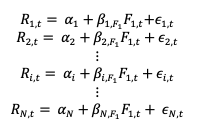
According to an examination of more than one year worth of market data, the size factor underperformed throughout the study period, most notably during the period of economic stress in the financial markets caused by the Covid-19 crisis. Given the crisis’s unprecedented severity, lockdown essentially shut down small and medium-sized firms, which finally suffered a period of catastrophic financial hardship, culminating in a non-negligible number of chain bankruptcies in the hardest-hit industries. This may help to explain why the Fever phase is the lowest-returning for the size factor. As the crisis progressed and governments spent billions on an accommodating monetary strategy to stimulate demand and re-establish healthy growth, size outperformed in the time after the pandemic’s fever phase (Figure 3).

ETFs to capture the Size factor

Let us recall that an Exchange-Traded Fund (ETF) is an investment vehicle that seeks to mirror the performance of a benchmark like an equity index and is traded on a continuous basis during the day like stocks. By investing in ETFs, an investor gains access to a plethora of diversification options through several asset classes (equity, bonds, currency, commodity, real estate, etc.).

Figure 3 illustrates the overall ETF distribution of the major providers of size factor ETFs in terms of percentage of asset under management. By examining the market overview for size factor investments, we can observe Blackrock and Vanguard dominance in this factor investing market, with 53.40% and 37.27% respectively, representing 90.67% of the overall size factor ETF market.

Figure 3. Size factor ETF market.
Size_factor_marketshare
Source: etf.com (2021).

Table 2 gives more detailed information about the biggest size factor ETF providers: the asset under management (AUM), expense ratio (ER) and the segment for the investments.

Table 2. Ranking of the biggest Size ETF providers.
Size_factor_actors
Source: etf.com (2021).

Why should I be interested in this post?

If you are an undergraduate or graduate student in a business school or at the university, you may have seen in your 101 finance course the CAPM related to the market factor. This post makes aware of the existence of another risk factor priced by the market.

If you are an investor, you may consider adding an exposure to size factor to enhance the overall portfolio return.

Related posts on the SimTrade blog

▶ Youssef LOURAOUI Minimum Volatility

▶ Youssef LOURAOUI Value Factor

▶ Youssef LOURAOUI Yield Factor

▶ Youssef LOURAOUI Momentum Factor

▶ Youssef LOURAOUI Quality Factor

▶ Youssef LOURAOUI Growth Factor

Useful resources

Academic research

Banz, R.W., 1981. The relationship between return and market value of common stocks. Journal of Financial Economics, 9: 3-18.

Basu, S., 1977. Investment performance of common stocks in relation to their price-earnings ratios: A test of Efficient Market Hypothesis. The Journal of Finance, 32: 663-682.

Fama, E.F., French, K.R. 1992. The Cross-Section of Expected Stock Returns. The Journal of Finance, 47: 427-465.

Fama, E.F., French, K.R., 2015. A five-factor asset pricing model. Journal of Financial Economics, 116(1): 1-22.

Hasaj, M., Sherer, B., 2021. Covid-19 and Smart-Beta: A Case Study on the Role of Sectors. EDHEC-Risk Institute Working paper.

Litzenberger, R., Ramaswamy, K., 1982. The Effects of Dividends on Common Stock Prices Tax Effects or Information Effects? The Journal of Finance, 37(2): 429-443.

Mangram, M.E., 2013. A simplified perspective of the Markowitz Portfolio Theory. Global Journal of Business Research, 7(1): 59-70.

Pagano, M., Wagner, C., Zechner, J., 2020. Disaster Resilience and Asset Prices, Working paper.

Reinganum, M., 1981. The Arbitrage Pricing Theory: Some Empirical Results. The Journal of Finance, 36(2): 313-321.

Business analysis

etf.com, 2021. Biggest Size Factor ETF providers.

MSCI Investment Research, 2021. Factor Focus: Size.

About the author

The article was written in September 2021 by Youssef LOURAOUI (ESSEC Business School, Global Bachelor of Business Administration, 2017-2021).

Momentum Factor

Momentum Factor

Youssef_Louraoui

In this article, Youssef LOURAOUI (ESSEC Business School, Global Bachelor of Business Administration, 2017-2021) presents the momentum factor, which is based on a risk factor that aims to get exposure to stocks that have a winning tendency in the upside and downside assuming that they will continue to do well in the short term.

Another similar concept related to momentum is trend following. It is a trading strategy that seeks to profit on an asset’s momentum in a certain direction. A trend occurs when the price moves in a consistent direction (upward or downward). Momentum investing and trading are based on the premise that prices respond to the strength of their supply and demand sources (at least in part) (Investopedia, 2021). It’s considered as a forward-looking strategy. Momentum manifests itself in a variety of different ways. It might be based on publicly traded firms’ earnings reports, the connection between buyers and sellers in the market, or even the usual pace of price rises and decreases in the past.

This article is structured as follows: we begin by defining the momentum factor and reviewing academic studies. The MSCI Momentum Factor Index, which is well used as a benchmark in the asset management industry, is next presented in terms of performance, risk-return trade-off, and behavior during the Covid-19 crisis. We showcase the ETF market for investors looking to profit from the momentum factor.

Definition

In the world of investing, a factor is any attribute that helps explain an asset’s long-term risk and return performance. In the late 1970s, the portfolio management industry’s objective was to capture the market return on a portfolio. As a result of Markowitz and Tobin’s earlier research, William Sharpe, John Lintner, and Jan Mossin independently developed the Capital Asset Pricing Model (CAPM). Because it enabled investors to properly value assets in terms of systematic risk, the CAPM was a significant evolutionary step forward in the theory of capital market equilibrium (Mangram, 2013).

Eugene Fama and Kenneth French, following the CAPM’s original work, developed the Fama-French three-factor model in 1993 to solve the CAPM’s inadequacies. It claims that, in addition to the market risk component of the CAPM, two other factors have an effect on the returns on securities and portfolios: market capitalization (called the “size” factor) and the book-to-market ratio (referred to as the “value” factor).
Other factor characteristics were developed to capture some additional performance as financial research advanced and significant contributions were made.

The Momentum factor refers to a winning stock’s tendency to continue doing well in the short term (Jegandeesh and Titman, 1993).

Academic research

The momentum premium was originally found by academics in 1993, when UCLA researchers Narasimhan Jegadeesh and Sheridan Titman proved that buying well-performing equities and selling underperforming ones provided large positive returns over three to twelve-month holding periods. The study finds that these techniques are profitable not because of their systematic risk or delayed stock price responsiveness to common causes. However, a portion of the anomalous returns achieved in the first year following portfolio creation fade away during the next two years. A similar pattern of returns is often observed around the earnings releases of previous winners and losers (Jegandeesh and Titman, 1993).

Empirical studies

Numerous subsequent research have established that the momentum factor exists across stock sectors, nations, and, more broadly, asset classes. Momentum is not as well understood as other variables, even though several theories seek to explain it. Some feel it is remuneration for taking on a high degree of risk, while others believe it is a result of market inefficiencies caused by delayed pricing reactions to firm-specific information.

While contrarian strategies have garnered much attention in recent academic research, the early work on market efficiency concentrated on relative strength strategies that invest in previous winners and sell past losers. Notably, Levy (1967) asserts that a trading method that purchases equities at prices significantly higher than their average price over the previous 27 weeks generates considerable anomalous profits. Jensen and Bennington (1970), on the other hand, note that Levy developed his trading rule after evaluating 68 alternative trading rules in his dissertation and express reservations about his results as a result (Jegandeesh and Titman, 1993). Jensen and Rennington examine the profitability of Levy’s trading rule over a lengthy period that falls mostly outside of Levy’s initial sample period. They discover that Levy’s trading rule does not outperform a buy and hold strategy throughout their sample period, and so ascribe Levy’s outcome to selection bias (Jegandeesh and Titman, 1993).

Economical interpretation

While the scholarly discussion has shifted away from relative strength trading rules, a lot of practitioners continue to utilize relative strength as a stock selection criterion. For example, Grinblatt and Titman (1989, 1991) found that most mutual funds purchased equities that had grown in price over the preceding quarter (Jegandeesh & Titman, 1993).

MSCI Momentum Factor Index

MSCI Factor Indexes are rules-based, transparent indexes that target equities with favorable factor qualities, as determined by academic discoveries and empirical outcomes, and are designed for easy implementation, replicability, and usage in both standard indexed and active portfolios. Momentum is classified as a “persistence” component, which means that it benefits from long-term market (MSCI Factor research, 2021). The MSCI Momentum Index measures:

  • Risk-adjusted excess return – that is, return that surpasses the benchmark – during a 6-month period
  • Risk-adjusted excess return that outperforms the benchmark over a 12-month period

These findings conclude in the research paper of Moskowitz et all (1999) hold up to a variety of criteria and treatments and provide critical practical insights into the profitability of momentum investing (Moskowitz, 1999). For example, these findings suggest that momentum strategies are not very well diversified, as both winners and losers typically come from the same industry. Additionally, if trading on momentum is desired, industry-based techniques tend to be more profitable and implementable. Unlike individual stock momentum techniques, which appear to be primarily driven by the sell side, industry momentum generates as much or more profit on the purchase side as on the sell side. Additionally, unlike individual stock momentum, sector momentum earnings continue to be robust among the largest, most liquid companies (Moskowitz, 1999).

Performance of the MSCI Momentum Factor Index

Figure 1 compares MSCI Momentum Factor Index performance to those of other factors from May 1999 to May 2020. All indices are rebalanced on a 100-point scale to ensure consistency in performance and to facilitate factor comparisons.

Figure 1. Performance of the MSCI Momentum Factor Index from 1999-2020.
Performance of the MSCI Momentum Factor Index from 1999-2020.
Source: MSCI Factor research (2021).

According to MSCI research, the momentum component has historically been one of the most effective generators of excess returns, consistently excelling in macro conditions characterized by a prolonged cycle in underlying market trends. As per the figure below, the MSCI World Momentum Index has historically generated excess returns over the long run, outperforming the MSCI World Index by 3.17 percent year since 1999 (MSCI Factor study, 2021).

Risk-return profile of MSCI Momentum Factor Index

Figure 2 shows the MSCI Momentum Factor Index compared to other factors over the period May 1999 – May 2020 in terms of risk/reward. The risk-return tradeoff states that the potential return rises with an increase in risk. Individuals connect low levels of uncertainty about future returns with low potential returns, while high levels of uncertainty or risk are associated with large potential returns. According to the risk-tradeoff trade-off, an investor’s money can generate higher returns only if the investor is willing to endure a higher risk of loss (Figure 2).

Figure 2. Risk-return profile of MSCI Momentum Factor Index compared to a peer group.
Risk-return profile of MSCI Momentum Factor Index compared to a peer group
Source: MSCI Factor research (2021).

Behavior of the MSCI Momentum Factor Index during the Covid-19 crisis

The Covid-19 crisis has not only caused significant social and economic suffering, but it had also an impact on financial markets. To study the behavior of the factors during the Covid-19 crisis, we compute the return of the MSCI Factor indexes during the different stages of the crisis. The MSCI Factor indexes are: value, size, quality, momentum and minimum volatility. Following Pagano et al. (2020) and Hasaj and Sherer (2021), we decompose the Covid-19 crisis into five stages: origin, incubation, outbreak, fever, and treatment. Each stage is described below.

  • Origin (01/11/2019 – 01/01/2020): the first instances are reported in Wuhan, China.
  • Incubation (02/01/2020 – 17/01/2020): during this phase, the number of patients began to rise at a faster rate, raising concerns about the disease’s severity.
  • Outbreak (20/01/2020 – 21/02/2020): the number of cases rose to the point that the World Health Organization (WHO) decided that this illness may pose a major threat to the world’s population, and the pandemic was proclaimed.
  • Fever (24/02/2020 – 20/03/2020): markets are extremely volatile, owing to government restrictions aimed at flattening the infection curve, with the decision to impose a lockdown in numerous nations as the most notable measures, among others.
  • Treatment (23/03/2020 – 15/04/2020): most of this turnaround occurs between March and June 2020, which corresponds with the start of good news about the discovery and widespread use of the vaccine.

Table 1 gives the performance of the MSCI factor indexes during the different stages of the Covid-19 crisis. Performance is measured by the return computed on the time-period of each stage, and then annualized for comparison across the different stages. We use data are from Thomson Reuters.

Table 1. Performance of the MSCI factor indexes during the Covid-19 crisis.
Performance of the MSCI factor indexes during the Covid-19 crisis
Source: computation by the author (data source: Thomson Reuters).

Both during the pre-lockdown phase (January 2nd to January 17th 2020) and during the post-lockdown phase (23 March 2020 – 15 April 2021), the momentum component performed well, attaining the second best risk/reward tradeoff (Table 1).

ETFs to capture the Momentum factor

Let us recall that an Exchange-Traded Fund (ETF) is an investment vehicle that seeks to mirror the performance of a benchmark like an equity index and is traded on a continuous basis during the day like stocks. By investing in ETFs, an investor gains access to a plethora of diversification options through several asset classes (equity, bonds, currency, commodity, real estate, etc.).

Figure 3 illustrates the overall ETF distribution of the major providers of momentum factor ETFs in terms of percentage of asset under management. By examining the market overview for momentum factor investments, we can observe Blackrock’s dominance (iShares), with assets under management underpinning $27 billion of the overall market value, holding 55% of the overall percentage of the benchmark retained.

Figure 3. Momentum factor ETF market.
 Momentum factor ETF market
Source: etf.com (2021).

Table 2 gives more detailed information about the biggest momentum factor ETF providers: the asset under management (AUM), expense ratio (ER) and the segment for the investments.

Table 2. Ranking of the biggest Momentum ETF providers.
Ranking of the biggest Momentum ETF providers
Source: etf.com (2021).

Why should I be interested in this post?

If you are an undergraduate or graduate student in a business school or at the university, you may have seen in your 101 finance course the CAPM related to the market factor. This post makes aware of the existence of an other risk factor priced by the market.

If you are an investor, you may consider adding an exposure to momentum factor to enhance the overall portfolio return.

Related posts on the SimTrade blog

   ▶ Youssef LOURAOUI Minimum Volatility

   ▶ Youssef LOURAOUI Value Factor

   ▶ Youssef LOURAOUI Yield Factor

   ▶ Youssef LOURAOUI Size Factor

   ▶ Youssef LOURAOUI Quality Factor

   ▶ Youssef LOURAOUI Growth Factor

Useful resources

Academic research

Fama, E.F. and French, K.R. (1992), The Cross-Section of Expected Stock Returns. The Journal of Finance , 47: 427-465.

Jegandeesh, N., Titman, S., 1993. Returns to buying winners and selling losers: Implication for stock market efficiency. The Journal of Finance , 48(1), 1-34.

Jensen, M. C., Benington, G. A. 1970. Random walks and technical theories: Some additional evidence. The Journal of Finance , 25: 469-482

Levy, R. A. 1967. Relative strength as a criterion for investment selection. The Journal of Finance , 22: 595-610.

Mangram, M. E., 2013. A simplified perspective of the Markowitz Portfolio Theory. Global Journal of Business Research , 7(1): 59-70.

Hasaj, M., Sherer, B., 2021. Covid-19 and Smart-Beta: A Case Study on the Role of Sectors. EDHEC-Risk Institute Working Paper, 1-35.

Pagano, M., Wagner, C., Zechner, J. 2020. Disaster Resilience and Asset Prices, Working paper.

Business analysis

etf.com, 2021. Biggest Momentum ETF providers.

MSCI Investment Research, 2021. Factor Focus: Momentum

Investopedia, 2021. The difference between Trends and Momentums

About the author

The article was written in September 2021 by Youssef LOURAOUI (ESSEC Business School, Global Bachelor of Business Administration, 2017-2021).

Yield Factor

Yield Factor

Youssef_Louraoui

In this article, Youssef LOURAOUI (ESSEC Business School, Global Bachelor of Business Administration, 2017-2021) presents the yield factor, which is based on a risk factor that aims to get exposure to companies that are regarded to be inexpensive and have a history of consistent and rising dividends.

This article is structured as follows: we begin by defining the yield factor and reviewing academic studies. The MSCI Yield Factor Index, which is well used as a benchmark in the asset management industry, is next presented in terms of performance and risk-return trade-off. We showcase the ETF market for investors looking to profit from the yield factor.

Definition

In the world of investing, a factor is any aspect that helps explain an asset’s long-term risk and return performance. In the late 1970s, the portfolio management industry’s objective was to capture the market return on a portfolio. As a result of Markowitz and Tobin’s earlier research, William Sharpe, John Lintner, and Jan Mossin independently developed the Capital Asset Pricing Model (CAPM). Because it enabled investors to properly value assets in terms of systematic risk, the CAPM was a significant evolutionary step forward in the theory of capital market equilibrium (Mangram, 2013).

Eugene Fama and Kenneth French, following the CAPM’s original work, developed the Fama-French Three-Factor model in 1993 to solve the CAPM’s inadequacies. It claims that, in addition to the market risk component of the CAPM, two other factors have an effect on the returns on securities and portfolios: market capitalization (called the “size” factor) and the book-to-market ratio (referred to as the “value” factor). Other factor characteristics were developed to capture some additional performance as financial research advanced and significant contributions were made.

The yield factor is based on a risk factor that aims to get exposure to companies that are regarded to be inexpensive and have a history of consistent and rising dividends (Arnott and Asness, 2003).

Academic research

Since 1995, and until a recent increase in response to plummeting earnings, market wide dividend-payout ratios in the United States had been in the lowest historical decile, reaching record lows between late 1999 and mid-2001. In other words, earnings retention rates have lately reached or above all-time highs (Arnott and Asness, 2003). Meanwhile, despite the dramatic decline in stock prices since early 2000, price-to-earnings and price-to-dividend ratios remain high by historical standards. With recent valuation ratios so high and dividend payouts so low, the only way future long-term stock returns can approach historical norms is if profits growth accelerates significantly. Certain market analysts, including several prominent Wall Street strategists, do predict extraordinary long-term growth. They attribute this confidence to a variety of factors, including previous policies of low dividend payment ratios. According to the financial literature (Arnott and Asness, 2003), the attractiveness for the yield factor could be explained by the following reasons:

  • Corporate executives are averse to dividend cuts. Perhaps a high payout ratio reflects managerial confidence in the future stability and increase of earnings, whilst a low payout ratio reflects the reverse. This confidence (or lack thereof) may be founded on public as well as private data
  • Another explanation compatible with the link we discovered experimentally is that businesses occasionally retain an excessive amount of revenue because of managers’ ambition to construct empires (Jensen, 1986). This conduct does not have to be malicious: A seemingly innocuous coincidence policy of profit retention may end up fostering empire development by accumulating an enticing cash hoard. On the other hand, while funding via share issue and paying significant dividends may be less tax effective, it may subject management to greater scrutiny, eliminate conflicts of interest, and so limit empire building

The article concluded that the empirical evidence supports a world in which managers possess private information that motivates them to pay out a large share of earnings when they are optimistic that dividend cuts will not be necessary and a small share when they are pessimistic, possibly to ensure that dividend payouts are maintained (Arnott and Asness, 2003). Alternatively, the findings match a scenario in which low payment ratios result in inefficient empire building and the backing of less-than-ideal initiatives and investments, resulting in subpar later growth, whereas high payout ratios result in more carefully selected enterprises (Arnott and Asness, 2003). Additionally, the tale of empire-building matches the first macroeconomic facts well. At the moment, these explanations are speculative; further work on distinguishing between conflicting narratives is necessary.

MSCI Yield Factor Index

MSCI Factor Indexes are rules-based, transparent indexes that target equities with favorable factor qualities, as determined by academic discoveries and empirical outcomes, and are designed for easy implementation, replicability, and usage in both standard indexed and active portfolios.

The MSCI Yield Factor Index concentrate on firms that pay a high dividend yield, but exclude those that lack dividend sustainability, consistency, and quality. It considers securities that fulfill these screening criteria (MSCI Factor research, 2021). Only those having a dividend yield more than 30% of the parent market capitalization index are included.

The yield factor is classified as a “defensive” component, which means that it has historically benefited from economic contraction. For several reasons, investors may be interested in the stock dividend income connected with the yield component. The method has been adopted by institutional investors seeking income outside of the fixed income industry. For example, an insurance business that requires a consistent revenue stream to cover claims may lean its portfolio toward the yield component to accomplish this goal. Additionally, historically, high dividends have accounted for a sizable share of long-term overall portfolio performance (MSCI Factor research, 2021).

Dividend investment is as ancient as stocks, having played a critical part in the growth of firms throughout history. Benjamin Graham and David Dodd, pioneering economists, memorably described dividend distributions as “the primary function of a corporate organisation… A successful business is one that can pay dividends on a consistent basis and, presumably, improve the rate over time” (MSCI Factor research, 2021).

Numerous ideas attempt to explain why high-dividend equities perform so well. One observes that yield investors have favored current dividend payouts above uncertain future capital returns. Additionally, they have viewed dividend increases as a predictor of future success (MSCI Factor research, 2021). Dividend yields have historically been good predictors of profit growth, according to several studies (MSCI Factor research, 2021). A naive high-yielding equity strategy may fall victim to a variety of “yield traps,” including those caused by momentarily high earnings, big dividends, or decreasing stock prices (MSCI Factor research, 2021).

Performance of the MSCI Yield Factor Index

Figure 1 compares the MSCI Yield Factor Index’s performance to those of other factors from May 1999 to May 2020. All indices are rebalanced on a 100-point scale to ensure consistency in performance and to facilitate factor comparisons.

Figure 1. Performance of the MSCI Yield Factor Index from 1999-2020.
Performance of the MSCI Yield Factor Index from 1999-2020
Source: MSCI Factor research (2021).

Since 1999, the MSCI Yield Factor Index has consistently earned excess gains of 0.15 percent per year above the MSCI World Index analysed (MSCI Factor research, 2021).

Risk-return profile of MSCI Yield Factor Index

Figure 2 shows the MSCI Yield Factor Index compared to other factors over the period May 1999 – May 2020 in terms of risk/reward. The risk-return trade-off states that the potential return rises with an increase in risk. Individuals connect low levels of uncertainty about future returns with low potential returns, while high levels of uncertainty or risk are associated with large potential returns. According to the risk-return trade-off, an investor’s money can generate higher returns only if the investor is willing to endure a higher risk of loss (Figure 2).

Figure 2. Risk-return profile of MSCI Yield Factor Index compared to a peer group.
Risk-return profile of MSCI Yield Factor Index compared to a peer group.
Source: MSCI Factor research (2021).

High-yield equity factor investing entails screening for dividends that are sustainable over time. With equity market involvement, it has generated yield income. The MSCI High Dividend Yield Indexes are designed to track the performance of firms that have historically paid steady and rising dividends while avoiding value traps. Outside of fixed income, yield seekers have found the equity yield factor index to have several attractive characteristics, including defensive income, a long-term positive risk premium, and diversification against other factors.

ETFs to capture the Yield factor

Let us recall that an Exchange-Traded Fund (ETF) is an investment vehicle that seeks to mirror the performance of a benchmark like an equity index and is traded on a continuous basis during the day like stocks. By investing in ETFs, an investor gains access to a plethora of diversification options through several asset classes (equity, bonds, currency, commodity, real estate, etc.).

Figure 3 illustrates the overall ETF distribution of the major providers of yield factor ETFs in terms of percentage of asset under management. By examining the market overview for minimal volatility factor investments, we can observe Vanguard’s dominance in this factor investing market with 53.46%, representing nearly 164 billion in term of market value in the of the overall yield factor ETF market retained in this benchmark.

Figure 3. Yield factor ETF market.
Yield factor ETF market
Source: etf.com (2021).

Table 1 gives more detailed information about the biggest yield factor ETF providers: the asset under management (AUM), expense ratio (ER) and the segment for the investments.

Table 1. Ranking of the biggest Yield ETF providers.
Ranking of the biggest Yield ETF providers
Source: etf.com (2021).

Why should I be interested in this post?

If you are an undergraduate or graduate student in a business school or at the university, you may have seen in your 101 finance course the CAPM related to the market factor. This post makes aware of the existence of another risk factor priced by the market.

If you are an investor, you may consider adding an exposure to yield factor to enhance the overall portfolio return.

Related posts on the SimTrade blog

   ▶ Youssef LOURAOUI Minimum Volatility

   ▶ Youssef LOURAOUI Value Factor

   ▶ Youssef LOURAOUI Size Factor

   ▶ Youssef LOURAOUI Momentum Factor

   ▶ Youssef LOURAOUI Quality Factor

   ▶ Youssef LOURAOUI Growth Factor

Useful resources

Academic research

Arnott, R. and Asness, C., 2003. Surprise! Higher Dividends = Higher Earnings Growth. Financial Analysts Journal, 59(1): 70-87.

Jensen, M., 1986. Agency Costs of Free Cash Flow, Corporate Finance, and Takeovers. The American Economic Review, 76(2): 323-329.

Hasaj, M., Sherer, B., 2021. Covid-19 and Smart-Beta: A Case Study on the Role of Sectors. EDHEC-Risk Institute Working Paper.

Mangram, M.E., 2013. A simplified perspective of the Markowitz Portfolio Theory.Global Journal of Business Research, 7(1): 59-70.

Pagano, M., Wagner, C., Zechner, J., 2020. Disaster Resilience and Asset Prices, Working paper.

Business analysis

etf.com, 2021. Biggest Yield ETF providers.

MSCI Investment Research, 2021. Factor Focus: Yield.

About the author

The article was written in September 2021 by Youssef LOURAOUI (ESSEC Business School, Global Bachelor of Business Administration, 2017-2021).

Value Factor

Value Factor

Youssef_Louraoui

In this article, Youssef LOURAOUI (ESSEC Business School, Global Bachelor of Business Administration, 2017-2021) presents the value factor, which is based on a risk factor that aims to get exposure to undervalued firms in relation to their industry competitors in order to benefit from the potential upside.

This article is structured as follows: we begin by defining the value factor and reviewing academic studies. The MSCI Value Factor Index, which is well used as a benchmark in the asset management industry, is next presented in terms of performance, risk-return trade-off, and behavior during the Covid-19 crisis. We showcase the ETF market for investors looking to profit from the value factor.

Definition

In the world of investing, a factor is any aspect that helps explain an asset’s long-term risk and return performance. In the late 1970s, the portfolio management industry’s objective was to capture the market return on a portfolio. As a result of Markowitz and Tobin’s earlier research, William Sharpe, John Lintner, and Jan Mossin independently developed the Capital Asset Pricing Model (CAPM). Because it enabled investors to properly value assets in terms of systematic risk, the CAPM was a significant evolutionary step forward in the theory of capital market equilibrium (Mangram, 2013). Eugene Fama and Kenneth French, following the CAPM’s original work, developed the Fama-French Three-Factor model in 1993 to solve the CAPM’s inadequacies. It claims that, in addition to the market risk component of the CAPM, two other factors have an effect on the returns on securities and portfolios: market capitalization (called the “size” factor) and the book-to-market ratio (referred to as the “value” factor). Other factor characteristics were developed to capture some additional performance as financial research advanced and significant contributions were made.

The value factor is based on a risk factor that aims to get exposure to undervalued firms in relation to their industry competitors in order to benefit from the potential upside (Graham, 1971).

Academic research

The most influential academic studies in the value investing literature may be traced back to Fama and French’s foundational work. In 1993, Eugene Fama and Kenneth French created the Fama-French Three-Factor model in response to the CAPM’s shortcomings. It claims that, in addition to the market risk component introduced by the CAPM, two more variables affect the returns on securities and portfolios: market capitalization (often referred to as “size”) and book-to-market ratio (referred to as the “value” factor). According to Fama and French, the primary justification for include these qualities is that both size and book-to-market (BtM) ratios are related to the business issuing the securities’ economic fundamentals (Fama and French, 1993).

Fama and French assert in 2014 that their initial 1993 three-factor model does not sufficiently explain for some observed discrepancies in anticipated returns. As a result, Fama and French added two more factors to their three-factor model: profitability and investment. These two elements are justified by the dividend discount model’s (DDM) theoretical implications, which assert that profitability and investment contribute to the explanation of the returns obtained from the HML element in the first model (Fama & French, 2015).

Business investors analysis

Benjamin Graham’s book: “The intelligent investor”

The cornerstone of value investing is the belief that low-cost stocks beat higher-cost firms over time. Value is a “pro-cyclical” element, which means that it has tended to gain during periods of economic boom. The seminal work on the value factor is undoubtedly the contribution of Benjamin Graham in his work “The intelligent investor”, one of the most adored and glorified books in finance and considered as a menhir of modern investment (Graham, 1971). According to the value investment approach, he considers that intelligence is not the most important parameter in investing. There’s evidence that a high IQ and a college degree aren’t enough to create a smart investor. Long-Term Capital Management L.P., a hedge fund operated by a squadron of mathematicians, computer scientists, and two Nobel Laureates in Economics (Myron Scholes and Robert C. Merton), lost more than $2 billion in a couple of weeks in 1998 on a massive bet that the bond market would return to “normal.” However, the bond market continued to become increasingly anomalous, and LTCM had borrowed so much money that its failure threatened to capsize the entire financial system. Graham’s work deconstructs several interesting notions that allow one to make a well-reasoned investment decision and to escape from the various cognitive biases that can lead to taking more dangerous positions in the markets (Graham, 1971). In a nutshell, among the most important points for a value investor are (Graham, 1971):

  • A stock is more than a ticker symbol; it’s a share of ownership in a real firm with a value apart from its share price. The stock market is a pendulum that swings back and forth between unjustified optimism (which pushes up stock prices) and unjustified pessimism (which drives down stock prices) (which makes them too cheap)
  • A savvy investor buys from pessimists and sells to optimists. The present price of an investment determines its future value. The higher the price you pay, the lower your return
  • No investor, no matter how careful they are, will ever eliminate the possibility of making a mistake. Only by adhering to Graham’s “margin of safety,” that is, never overpaying for an investment, no matter how attractive it seems, can you decrease your odds of making a mistake
  • The key to financial success is personal growth in terms of how an investor reacts to market events without including emotions in the decision-making process, as this has a negative impact

Benjamin Graham and David Dodd’s book: “Security Analysis”

With the release of Security Analysis in 1934, Benjamin Graham and David Dodd permanently altered the philosophy and practice of investing. The United States, and indeed the rest of the globe, was engulfed in the Great Depression, a period of unprecedented financial turmoil (Graham & Dodd, 2010). The authors replied with a thorough modification in 1940. Many investors regard the second edition of Security Analysis to be the ultimate word from the most prominent investing philosophers of our time. Security Analysis is still considered the standard text for stock and bond analysis across the world. The work of Graham with “The Intelligent Investor” and “Security Analysis” is regarded as the “bible” of value investing. In a nutshell, the book describes the following aspects (Graham & Dodd, 2010):

  • The purpose of security analysis is to provide critical information about a stock or bond in an informative and useful manner to a prospective owner; and to make accurate judgments about a security’s safety and attractiveness relative to its current price range based on facts and criteria.
  • Graham and Dodd describe investing as follows: “An investment activity is one that, after careful analysis, guarantees the safety of money and an acceptable rate of return.” Speculative operations are those that do not comply with these requirements”.
  • Investors are classified into two types: those who are defensive and those who are adventurous. The former’s portfolio is comprised of a diverse selection of high-price stocks purchased at a discount. The entrepreneurial investor understands the value between market and intrinsic value, which enables him or her to analyze specific stocks in type of and profit from price-to-value discrepancies.
  • An analysis of a security involves two distinct types of factors: quantitative and qualitative. The former domain should encompass capital structure, earnings power, dividend distributions, and operational effectiveness. The qualitative domain is more ‘fluffy’; it encompasses the ‘character’ of the business, its market position(s), and an appraisal of the management team, among other things. Quantitative data is only useful when accompanied by qualitative analysis.
  • The most critical word in the book is “earnings power.” The authors emphasize the significance of estimating a company’s real future earnings based on its historical earnings (adjusted for one-time events) as well as its vulnerability to factors such as cyclical swings.

Example of a “value” stock

A value stock is one that trades at a lower price than the company’s actual performance. Because the price of the underlying shares may not reflect the company’s performance, value stock investors seek to profit from market inefficiencies (Investopedia, 2021). Value stocks, for example, include big money center banks. JPMorgan Chase & Co. (JPM) is a value stock that trades at a substantial discount to the market based on earnings.

MSCI Value Factor Index

MSCI Factor Indexes are rules-based, transparent indexes that target equities with favorable factor qualities, as determined by academic discoveries and empirical outcomes, and are designed for easy implementation, replicability, and usage in both standard indexed and active portfolios. The stock price as a multiple of business earnings, the price as a multiple of dividends paid, the price as a multiple of book value, and other “ratio descriptors” are all examples of value. Academics and investors disagree on which business best symbolizes a value company, resulting in a market potential for a range of investment products. On a sector-by-sector basis, the MSCI Enhanced Value Index uses three valuation ratio descriptors:

  • Forward price to earnings (Fwd P/E)
  • Enterprise value/operating cash flows (EV/CFO)
  • Price to book value (P/B)

The index tries to avoid the problems of value investing, such as “value traps,” or stocks that look inexpensive but do not grow in value. The research demonstrates that whole-firm valuation metrics like enterprise value have decreased concentration in highly leveraged businesses (those that have taken on a lot of debt).

Performance of the MSCI Value Factor Index

Figure 1 compares the MSCI Value Factor Index’s performance to those of other factors from May 1999 to May 2020. All indices are rebalanced on a 100-point scale to ensure consistency in performance and to facilitate factor comparisons.

Figure 1. Performance of the MSCI Value Factor Index from 1999-2020.
Performance of the MSCI Value Factor Index from 1999-2020
Source: MSCI Factor research (2021).

Since 1999, the MSCI World Enhanced Value Index has achieved excess returns above the MSCI World Index, with a 1.99 percent annual return over the MSCI World Index as seen above. (MSCI Factor research, 2021).

Risk-return profile of MSCI Value Factor Index

Figure 2 shows the MSCI Value Factor Index compared to other factors over the period May 1999 – May 2020 in terms of risk/reward. The risk-return tradeoff states that the potential return rises with an increase in risk. Individuals connect low levels of uncertainty about future returns with low potential returns, while high levels of uncertainty or risk are associated with large potential returns. According to the risk-tradeoff trade-off, an investor’s money can generate higher returns only if the investor is willing to endure a higher risk of loss (Figure 2).

Figure 2. Risk-return profile of MSCI Value Factor Index compared to a peer group.
Performance of the MSCI Value Factor Index from 1999-2020
Source: MSCI Factor research (2021).

The basis of value investing is identifying stocks whose prices appear to understate their fundamental worth. While many institutional investors may agree, value-index strategies are executed in a number of ways. Incorporating the value factor into a portfolio might potentially boost returns and function as a well-researched performance vector (MSCI Factor research, 2021).

Behavior of the MSCI Value Factor Index during the Covid-19 crisis

The Covid-19 crisis has not only caused significant social and economic suffering, but it had also an impact on financial markets. To study the behavior of the factors during the Covid-19 crisis, we compute the return of the MSCI Factor indexes during the different stages of the crisis. The MSCI Factor indexes are: value, size, quality, momentum and minimum volatility. Following Pagano et al. (2020) and Hasaj and Sherer (2021), we decompose the Covid-19 crisis into five stages: origin, incubation, outbreak, fever, and treatment. Each stage is described below.

  • Origin (01/11/2019 – 01/01/2020): the first instances are reported in Wuhan, China.
  • Incubation (02/01/2020 – 17/01/2020): during this phase, the number of patients began to rise at a faster rate, raising concerns about the disease’s severity.
  • Outbreak (20/01/2020 – 21/02/2020): the number of cases rose to the point that the World Health Organization (WHO) decided that this illness may pose a major threat to the world’s population, and the pandemic was proclaimed.
  • Fever (24/02/2020 – 20/03/2020): markets are extremely volatile, owing to government restrictions aimed at flattening the infection curve, with the decision to impose a lockdown in numerous nations as the most notable measures, among others.
  • Treatment (23/03/2020 – 15/04/2020): most of this turnaround occurs between March and June 2020, which corresponds with the start of good news about the discovery and widespread use of the vaccine.

Table 1 gives the performance of the MSCI factor indexes during the different stages of the Covid-19 crisis. Performance is measured by the return computed on the time-period of each stage, and then annualized for comparison across the different stages. We use data are from Thomson Reuters.

Table 1. Performance of the MSCI factor indexes during the Covid-19 crisis.
Performance of the MSCI factor indexes during the Covid-19 crisis
Source: computation by the author. Data source: Thomson Reuters.
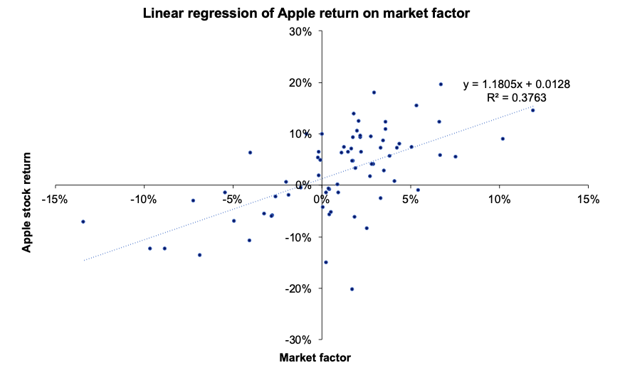
The value factor has performed not quite well in comparison to the other factors, finishing fourth out of five throughout the time period studied. Additionally, our study demonstrates that the value factor was the poorest performer during the incubation and outbreak stages and the second worst performer during the fever stage. This demonstrates the value factor’s instability during the Covid-19 crisis, which acted as a stress test.

ETFs to capture the Value factor

Let us recall that an Exchange-Traded Fund (ETF) is an investment vehicle that seeks to mirror the performance of a benchmark like an equity index and is traded on a continuous basis during the day like stocks. By investing in ETFs, an investor gains access to a plethora of diversification options through several asset classes (equity, bonds, currency, commodity, real estate, etc.).

Figure 3 gives the overall ETF distribution of the major providers of value factor ETFs in terms of asset under management. By examining the market overview for minimal volatility factor investments, we can observe Blackrock (iShares) and State Street Global Advisors as the most dominant players in this segment. They hold nearly 50% and 34% respectively of the overall value factor ETF market, which underpins nearly 117B$ of the overall 138B$ in terms of market value for the value factor ETF market retained in this benchmark.

Figure 3. Value factor ETF market.
Value factor ETF market
Source: etf.com (2021).

Table 2 gives more detailed information about the biggest value factor ETF providers: the asset under management (AUM), expense ratio (ER) and the segment for the investments.

Table 2. Ranking of the biggest Value ETF providers.
Ranking of the biggest Value ETF provider
Source: etf.com (2021).

Why should I be interested in this post?

If you are an undergraduate or graduate student in a business school or at the university, you may have seen in your 101 finance course the CAPM related to the market factor. This post makes aware of the existence of another risk factor priced by the market.

If you are an investor, you may consider adding an exposure to value factor to enhance the overall portfolio return.

Related posts on the SimTrade blog

   ▶ Youssef LOURAOUI Minimum Volatility

   ▶ Youssef LOURAOUI Size Factor

   ▶ Youssef LOURAOUI Yield Factor

   ▶ Youssef LOURAOUI Momentum Factor

   ▶ Youssef LOURAOUI Quality Factor

   ▶ Youssef LOURAOUI Growth Factor

Useful resources

Academic articles

Fama, E.F. French, K.R., 1992. The Cross-Section of Expected Stock Returns. The Journal of Finance , 47: 427-465.

Fama, E.F. French, K.R., 2015. A five-factor asset pricing model, Journal of Financial Economics , 116(1): 1-22.

Graham, B., Dodd, D., 1934. Security Analysis. 6th Edition, McGraw Hill.

Graham, B., 1949. The Intelligent Investor. 4th edition, Harper Business Essentials.

Hasaj, M., Sherer, B., 2021. Covid-19 and Smart-Beta: A Case Study on the Role of Sectors”. EDHEC-Risk Institute Working Paper.

Mangram, M.E., 2013. A simplified perspective of the Markowitz Portfolio Theory. Global Journal of Business Research, 7(1): 59-70.

Pagano, M., Wagner, C., Zechner, J. 2020. Disaster Resilience and Asset Prices, Working paper.

Business analysis

etf.com, 2021. Biggest Value Factor ETF providers.

MSCI Investment Research, 2021. Factor Focus: Value

Investopedia, 2021. Value Stock Definition.

About the author

The article was written in September 2021 by Youssef LOURAOUI (ESSEC Business School, Global Bachelor of Business Administration, 2017-2021).

Minimum Volatility Factor

Minimum Volatility Factor

Youssef_Louraoui

In this article, Youssef LOURAOUI (ESSEC Business School, Global Bachelor of Business Administration, 2017-2021) presents the Minimum Volatility Factor, which is based on a risk factor that aims to get exposure to securities with a low volatility profile as measured by beta compared to the market, as well as a low correlation with other assets.

This article is structured as follows: we begin by defining the minimum volatility factor and reviewing academic studies. The MSCI Minimum Volatility Factor Index, which is well used as a benchmark in the asset management industry, is next presented in terms of performance, risk-return trade-off, and behavior during the Covid-19 crisis. We showcase the ETF market for investors looking to profit from the minimum volatility factor.

Definition

In the world of investing, a factor is any aspect that helps explain an asset’s long-term risk and return performance. In the late 1970s, the portfolio management industry’s objective was to capture the market return on a portfolio. As a result of Markowitz and Tobin’s earlier research, William Sharpe, John Lintner, and Jan Mossin independently developed the Capital Asset Pricing Model (CAPM). Because it enabled investors to properly value assets in terms of systematic risk, the CAPM was a significant evolutionary step forward in the theory of capital market equilibrium (Mangram, 2013).

Eugene Fama and Kenneth French, following the CAPM’s original work, developed the Fama-French Three-Factor model in 1993 to solve the CAPM’s inadequacies. It claims that, in addition to the market risk component of the CAPM, two other factors have an effect on the returns on securities and portfolios: market capitalization (called the “size” factor) and the book-to-market ratio (referred to as the “value” factor). Other factor characteristics were developed to capture some additional performance as financial research advanced and significant contributions were made.

Minimum volatility is based on a risk factor that aims to get exposure to securities with a low volatility profile as measured by beta compared to the market, as well as a low correlation with other assets (MSCI Factor research, 2021).

Academic research

In the late 1970s, the portfolio management industry aimed to capture the market portfolio return, but as financial research advanced and certain significant contributions were made, this gave rise to other factor characteristics to capture some additional performance. The financial literature has long advocated for taking on more risk to get a better rate of return. This, however, is a widespread misunderstanding among investors. While extremely volatile equities can deliver spectacular gains, scholarly research has consistently demonstrated that low-volatility companies deliver superior risk-adjusted returns over time. This phenomenon is referred to as the “low volatility anomaly”, and that is why many long-term investors include low volatility factor strategies in their portfolios. This strategy is consistent with Henry Markowitz’s famous 1952 article, in which he preaches the virtues of asset diversification to construct a portfolio that provides the greatest balanced return in a risk-reward framework.

Empirical studies

Figure 1 represents the Markowitz Efficient Frontier, where all the efficient portfolios lie on the upper line. The efficient frontier is a collection of optimum portfolios that provide the highest expected return for a specified level of risk or the lowest risk for a specified level of return. Portfolios that fall below the efficient frontier are suboptimal because they do not provide a sufficient rate of return relative to the degree of risk (Figure 1).

Figure 1. Markowitz Efficient Frontier
Minimum volatility and Markowitz Efficient Frontier
Source: calculations done by the author

Economic interpretation

The term ‘Risk-Reward trade-off’ alludes to Markowitz’s core principle that the riskier an investment, the greater the required potential return. Investors will typically keep a risky investment only if the anticipated return is sufficiently high to compensate them for incurring the risk. Risk is the risk that the actual return on an investment will be less than expected, which is technically defined by standard deviation. A higher standard deviation indicates a greater risk and, thus, a greater potential return. Investors that are willing to take on risk expect to receive a risk premium. The term “risk premium” refers to “the expected return on an investment that is more than the risk-free rate of return”. The greater the risk, the greater the risk premium required by investors.

MSCI Minimum Volatility Factor Index

MSCI Factor Indexes are rules-based, transparent indexes that target equities with favorable factor qualities, as determined by academic discoveries and empirical outcomes, and are designed for easy implementation, replicability, and usage in both standard indexed and active portfolios. The MSCI Minimum Volatility Indexes are created by optimizing a set of sector, country, and factor restrictions to generate an index with the least overall volatility while also maintaining index replicability and investability. The major ways to executing a minimal volatility strategy fall into two categories in terms of methodology: (1) straightforward rank and selection and (2) optimization-based solutions (MSCI Factor research, 2021).

A straightforward technique rates the universe of stocks by anticipated volatility, then picks a subset of the members from the universe and applies a weighting mechanism. The connection between stock returns, which can have a major influence on the overall volatility strategy, is typically ignored in these techniques. While a basic rank and selection technique represents individual stock volatility, optimization-based approaches take into consideration both volatility and correlation effects, or the size and degree to which stocks move in lockstep (MSCI Factor research, 2021).

A naïve unconstrained minimal volatility strategy, on the other hand, has its own set of difficulties, including biases toward certain sectors and nations, undesirable factor exposures, and possibly excessive rebalancing turnover. However, well-designed optimizations with properly defined restrictions may be able to compensate for these flaws. Minimum volatility is classified as a conservative factor, which means that it has tended to benefit from periods of economic contraction. This type of strategy is more concerned with managing volatility than maximizing gains. In this sense, this strategy has produced a premium over the market for long periods, contradicting the principle that investors should not be rewarded with higher risk-adjusted returns for taking less risk than the market (MSCI Factor research, 2021).

The key objective of a minimum volatility strategy is to capture regional and global exposure to potentially less risky stocks. Historically, the MSCI Minimum Volatility Factor Index, for instance, have achieved lower volatility and lower drawdowns (peak-to-trough declines) relative to their factor counterparts during major market downturns (MSCI Factor research, 2021).

Tactical investors have employed MSCI Minimal Volatility Factor Index to decrease risk during market downturns while maintaining equity exposure. The minimum volatility premium was found in the early 1970s by economist Fischer Black coupled with the pioneer work of Portfolio construction of Henry Markowitz in 1952. and built on by others subsequently. After that, according to one idea, investors underpay for low volatility equities because they perceive them to be less lucrative, while overpaying for high volatility equities because they are seen as long-shot prospects for bigger profits. An alternative scholarly argument contends that investors might be overconfident in their abilities to predict the future, and that their views diverge more for high volatility equities, which have fewer predictable outcomes, resulting in increased volatility and poorer returns (MSCI Factor research, 2021).

Performance of the MSCI Minimum Volatility Factor Index

Figure 2 compares the MSCI Minimum Volatility Factor Index’s performance to those of other factors from May 1999 to May 2020. All indices are rebalanced on a 100-point scale to ensure consistency in performance and to facilitate factor comparisons.

Figure 2. Performance of the MSCI Minimum Volatility Factor Index from 1999-2020.
Minimum_volatility_performance
Source: MSCI Factor research, 2021.

With a 1.16% percent yearly return over the MSCI World Index since 1999, the MSCI World Minimum Volatility (USD) Index has consistently provided excess profits over the long run while maintaining a profile of risk among the most conservative of the peer group analysed (MSCI Factor research, 2021).

Risk-return profile of MSCI Minimum Volatility Factor Index

Figure 3 shows the MSCI Minimum Volatility Factor Index compared to other factors over the period May 1999 – May 2020 in terms of risk/reward. The risk-return tradeoff states that the potential return rises with an increase in risk. Individuals connect low levels of uncertainty about future returns with low potential returns, while high levels of uncertainty or risk are associated with large potential returns. According to the risk-tradeoff trade-off, an investor’s money can generate higher returns only if the investor is willing to endure a higher risk of loss (Figure 3).

Figure 3. Risk-return profile of MSCI Minimum Volatility Factor Index compared to a peer group.
Minimum_volatility_riskreturn
Source: MSCI Factor research, 2021.

Behavior of the MSCI Minimum Volatility Factor Index during the Covid-19 crisis

The Covid-19 crisis has not only caused significant social and economic suffering, but it had also an impact on financial markets. To study the behavior of the factors during the Covid-19 crisis, we compute the return of the MSCI Factor indexes during the different stages of the crisis. The MSCI Factor indexes are: value, size, quality, momentum and minimum volatility. Following Pagano et al. (2020) and Hasaj and Sherer (2021), we decompose the Covid-19 crisis into five stages: origin, incubation, outbreak, fever, and treatment. Each stage is described below.

  • Origin (01/11/2019 – 01/01/2020): the first instances are reported in Wuhan, China.
  • Incubation (02/01/2020 – 17/01/2020): during this phase, the number of patients began to rise at a faster rate, raising concerns about the disease’s severity.
  • Outbreak (20/01/2020 – 21/02/2020): the number of cases rose to the point that the World Health Organization (WHO) decided that this illness may pose a major threat to the world’s population, and the pandemic was proclaimed.
  • Fever (24/02/2020 – 20/03/2020): markets are extremely volatile, owing to government restrictions aimed at flattening the infection curve, with the decision to impose a lockdown in numerous nations as the most notable measures, among others.
  • Treatment (23/03/2020 – 15/04/2020): most of this turnaround occurs between March and June 2020, which corresponds with the start of good news about the discovery and widespread use of the vaccine.

Table 1 gives the performance of the MSCI factor indexes during the different stages of the Covid-19 crisis. Performance is measured by the return computed on the time-period of each stage, and then annualized for comparison across the different stages. We use data are from Thomson Reuters.

Table 1. Performance of the MSCI factor indexes during the Covid-19 crisis.
Performance of the MSCI factor indexes during the Covid-19 crisis
Source: computation by the author (Data source: Thomson Reuters).

One conclusion that can be drawn from our research supports the reason for the minimal volatility strategy, namely, to minimize portfolio volatility by keeping limited exposure to highly volatile stocks. In this respect, the Covid-19 pandemic period served as a significant stress test for this strategy, which outperformed the other return factors in the period preceding and following worldwide containment, with a risk-reward trade-off much higher than the average of the chosen factors.

ETFs to capture the Minimum Volatility factor

Let us recall that an Exchange-Traded Fund (ETF) is an investment vehicle that seeks to mirror the performance of a benchmark like an equity index and is traded on a continuous basis during the day like stocks. By investing in ETFs, an investor gains access to a plethora of diversification options through several asset classes (equity, bonds, currency, commodity, real estate, etc.).

Figure 4 gives the overall ETF distribution of the major providers of minimal volatility factor ETFs in terms of asset under management. By examining the market overview for minimal volatility factor investments, we can observe Blackrock ETFs (iShares) dominance, with 78.43% of the overall minimum volatility factor ETF market. This represents roughly 47B$ of the overall minimum volatility market retained for this benchmark.

Figure 4. Minimum Volatility factor ETF market.
 Minimum Volatility factor ETF market
Source: etf.com, 2021.

Table 2 gives more detailed information about the biggest minimum volatility factor ETF providers: the asset under management (AUM), expense ratio (ER) and 3-month total return (3-Mo TR) and the segment for the investments.

Table 2. Ranking of the biggest Minimum Volatility ETF providers.
 Minimum Volatility factor ETF market actors
Source: etf.com, 2021.

Why should I be interested in this post?

You may have seen the CAPM linked to the market factor in your 101 finance course if you are an undergraduate or graduate student at a business school or university. This article raises awareness of the presence of other additional risk factors.

If you’re an investor, you might want to explore increasing your exposure to the minimum volatility factor to boost your portfolio’s total return.

Related posts on the SimTrade blog

   ▶ Youssef LOURAOUI Size Factor

   ▶ Youssef LOURAOUI Value Factor

   ▶ Youssef LOURAOUI Yield Factor

   ▶ Youssef LOURAOUI Momentum Factor

   ▶ Youssef LOURAOUI Quality Factor

   ▶ Youssef LOURAOUI Growth Factor

Useful resources

Academic research

Markowitz, H., 1952. Portfolio Selection. The Journal of Finance, 7(1): 77-91.

Mangram, M.E., 2013. A simplified perspective of the Markowitz Portfolio Theory. Global Journal of Business Research, 7(1): 59-70

Hasaj, M., Sherer, B., 2021. Covid-19 and Smart-Beta: A Case Study on the Role of Sectors. EDHEC-Risk Institute Working Paper.

Pagano, M., Wagner, C., Zechner, J. 2020. Disaster Resilience and Asset Prices, Working paper.

Business analysis

etf.com, 2021. Biggest Minimum Volatility ETF providers.

MSCI Investment Research, 2021. Factor Focus: Volatility.

About the author

The article was written in September 2021 by Youssef LOURAOUI (ESSEC Business School, Global Bachelor of Business Administration, 2017-2021).

Repo Rate

Repo Rate

Shruti CHAND

In this article, Shruti CHAND (ESSEC Business School, Grande Ecole Program – Master in Management, 2020-2022) elaborates on the concept of repo rate.

This read will help you get started with understanding repo rate and its significance.

What is Repo?

Repurchase rate is the rate at which the financial institutions in a country borrow and lend assets amongst themselves for a short-term. In the interbank market, the underlying security is sold by a bank to another in exchange of buying it the next day at a higher price on the following day usually. This exchange of the asset is facilitated by a contract known as “Repurchase agreement at a rate” or more commonly referred to “Repo”.

This agreement is similar to a loan agreement where the borrower of the loan pledges collateral with the lender for the time it borrows money and claims it back when the loan agreement is fulfilled. The underlying asset is usually a money market instrument such as Treasury bills and Treasury bonds. The main criteria to qualify as a collateral is that it should be liquid so that it can be sold in the open market if required.

Let us understand how a repurchase agreement works in detail:

The party of the contract who lends money in exchange of interests is known as the “repo seller”.

The borrower of the loan is known as the “repo buyer”.

The rate of the loan at which the lending is facilitated is known as the “repo rate”.

The collateral allows the lender to be protected against counter-party risk of the borrower. The value of the collateral is always higher than the amount lent to provide protection against market risk associated with collateral value. This additional amount is known as “haircut”.

Example

Let us illustrate this concept with an example:

Let us say Bank A (the borrower) is in dire need of liquid cash to facilitate an important transaction. In this scenario, it will turn to the Bank B (the lender) and request an amount of $100 m in cash.

Both banks decide to sign a repurchase agreement to facilitate this request. Bank B agrees to lend $100 m to Bank A and in return, Bank A agrees to pledge to Bank B Treasury bonds of a value higher than the value lent. This additional amount is known as ‘haircut’ as mentioned above. Let us assume in this case the haircut is $20 m, then the value of collateral that Bank A will keep for Bank B is equal to $120 m.

On day one, a repurchase agreement is signed between both banks. Bank A facilitates the agreement by holding the asset collateral with itself and Bank B lends cash to Bank A for its operations.

On day two, Bank A repays to Bank B the borrowed amount of $100 m and interests computed with the repo rate over one day. Let us assume the repo rate is equal to 5%. In this case, Bank A will pay $13,888 of interests to Bank B on day two and Bank B will free the collateral to Bank A.

Now that you understand a repo transaction, what is important also is to understand that a repo is one of the very important sources of funding for financial institutions in an economy. Central banks in every country use repurchase agreements to maintain liquidity level in the economy.

For example, the European Central Bank (ECB) sets three rates to keep the prices stable in the Euro zone. One of these rates is known as Refinancing option or Repurchasing option, which is an agreement to repurchase the collateral that the banks keep with the ECB of the country to borrow money for a very short period of time. Banks keep their Treasury bills or eligible securities with the Central Bank in exchange of money, they buy it later at a fixed price. ECB sets this rate every six weeks. This is how the policy makers for the Euro zone control the inflation level within the economy. On the other hand, opposite measures will be taken when the Central Bank needs to pump money in the economy.

Final Words

Repo rates are crucial to every economy and it differs based on various factors and is taken in control by policy makers whenever needed. As a student curious about Finance, learning about Repo Rate will go a long way in the future to understand better how liquidity and prices in the economy is maintained.

Relevance to the SimTrade certificate

This post deals with Repo Rate and how it is managed in the EU zone context.

About theory

  • By taking the SimTrade course , you will learn more about the markets. It’s important to remember that lending is a crucial part for investing.

Take SimTrade courses

About practice

  • By launching the series of Market maker simulations, you can extend your learning about financial markets and trading approaches.

Take SimTrade courses

About the author

Article written in August 2021 by Shruti CHAND (ESSEC Business School, Grande Ecole Program – Master in Management, 2020-2022).

Balance of Trade

Balance of Trades

Shruti CHAND

In this article, Shruti CHAND (ESSEC Business School, Grande Ecole Program – Master in Management, 2020-2022) elaborates on the concept of balance of trade.

This read will help you get started with understanding balance of trade and how it is practiced in today’s world.

Introduction

Balance of trade (BOT) refers to the difference between the monitory value of a country’s imports and exports over a specific period of time.

Imports refers to goods and services produced by another country and purchased by the domestic country for its consumption purposes whereas exports refer to the sale of goods and services produced by the domestic country to another country.

Balance of trade is the biggest part of the balance of payment (BOP). Balance of payment is the sum total of all the economic transactions of the residents of the country with the rest of the world. It includes capital movements, loan repayments, tourism, freight and insurance charges, and other payments. The payments and receipts of each country must be equal where any apparent quality simply leaves one country acquiring assets in the other.

Coming back to the balance of trade (also known as the ‘trade balance’, ‘international trade balance’, ‘commercial balance’ or the ‘net exports’) can result in a surplus (exports > imports) or in a deficit (imports > exports). When the exports of a country exceed its imports, the country is said to have a trade surplus. When the imports of a country exceed its exports, the country is said to have a trade deficit.

There have been constant changes in the economic theories revolving around
the balance of trade. According to the theory of mercantilism, a favorable/surplus balance of trade was necessary for ensuring the growth and well-being of an economy. It also symbolized a country’s wealth and power. However, this theory was soon challenged by classical economic theory of the late 18 th century when economists such as Adam Smith argued that free trade is more beneficial than the tendencies of mercantilism. The classical theory argued that countries are not quired to maintain a surplus in order to be more beneficial that is because a continuing surplus might in fact represent the underutilization of resources that could have otherwise contributed towards the country’s wealth.

Generally, developing countries have difficulty maintaining surpluses since the terms of trade during periods of recession are unfavorable for them. This is because they have to pay comparatively higher prices for finished goods that they import but receive lower prices for their exports of raw material or unfurnished goods.

Calculation of the Balance of Trade

The balance of trade is simply calculated as exports minus imports. It can be represented as follows:

TB = X – M where,

TB = Trade Balance
X = Exports (value of goods and services sold to the rest of the world)
M = Imports (value of goods and services purchased by the rest of the world)

When the exports are greater than imports it results in a trade surplus whereas when imports are greater than exports it results in a trade deficit. A country with a large trade deficit generally borrows money from other countries to balance the trade deficit while a country with large trade suppliers lends money to other nation for investing purposes. Generally, on a surface level, surplus is preferable to a deficit. But in reality, this might be an oversimplification. This is because a trade deficit might not inherently be bad,
as it can be an indicator of a strong economy. In addition to this, when we combine practical and sensible investment decisions, a deficit may lead to the stronger economic growth of a country in the future.

Interpretation for an Economy

In a basic sense, economists use balance of trade to measure the relative strength of a country’s economy. A country where imports are greater than exports face a trade deficit whereas a country where exports are greater than imports face a trade surplus.

But the reality of a situation is different when it comes to the interpretation of an economy based on the balance of trade. Sometimes a trade deficit can be unfavorable for a nation that focuses a lot on the export of raw material. As a result, this type of economy usually imports a lot of consumer products. As a consequence of the scene, the domestic businesses don’t attain the experiences needed to compete in the international market. Instead, the economy becomes increasingly dependent on global commodity prices, which can be highly volatile for such economy. Sometimes countries adopt the complete opposite of trade deficit when they follow the theory of mercantilism. In this scenario countries believe in maintaining a continuous surplus of trade in order to achieve the growth of the economy. It indulges in protective measures such as tariffs and import quotas to ensure the same. As a result, such measures can facilitate for a trade surplus, but a continuous trade surplus might result in higher cost for consumers, reduce international trade and may lead to diminishing economic growth.

Therefore, a positive or negative trade balance done does not necessarily indicate a healthy or a weak economy. Whether a trade surplus/deficit is beneficial for an economy or not depends on multiple factors such as the countries involved, trade policy decisions, the duration of the trade surplus/deficit, the size of the trade imbalance etc. For example, business cycles are an important factor to consider while interpreting the balance of trade. Because, in a recession, and economy tries to create more jobs and demand in the economy and as a result prefers to export more. On the contrary, during an economic expansion, countries prefer to import to promote price competition and as a direct consequence to limit inflation.

Related posts on the SimTrade blog

   ▶ Bijal GANDHI Economic indicators

   ▶ Bijal GANDHI Gross Domestic Product (GDP)

About the author

Article written by Shruti CHAND (ESSEC Business School, Grande Ecole Program – Master in Management, 2020-2022).

Online Brokers

Online Brokers

Shruti CHAND

In this article, Shruti CHAND (ESSEC Business School, Grande Ecole Program – Master in Management, 2020-2022) elaborates on the concept of online brokers.

This read will help you get started with understanding online brokers and how it is practiced in today’s world.

Introduction

A stockbroker is an entity that facilitates trading, that is to say executing trades on your behalf and storing your cash and stocks with them. Traditionally, brokers have been big banks and financial institutions that deal with billions of dollars in trading volumes. With advancing technology around the world, financial markets is adapting to the change, allowing retail investors to invest in the financial markets in new ways.

An online broker essentially is an entity that carries the activity of a broker without having a brick and motor existence, allowing its customers to execute and manage their trades by themselves on a trading platform available on the internet.

An online broker allows investors to trade in stocks, derivatives, commodities, cryptocurrencies, exchange-traded funds (ETFs), etc. in multiple currencies and markets. Additionally, they provide additional services such as:

  •  Market news
  •  Extensive investment information
  •  Expert advice
  •  Technical and fundamental analysis

online brokers provide their services in return of transactions and management fees, which are on the lower side for brokerage firms because of the low cost, they incur because of their non-physical existence. The expenses related to labor, property, management systems are reduced as all the process is carried out digitally. This allows the customers/investors to have quick transactions and a smooth experience. Some online brokers are in fact divisions of larger traditional brokers, e.g. Saxo Bank.

How can you use an online broker?

There are various online brokers available in every country which will allow you to use their platforms via their mobile phone application or internet website. Just as traditional brokers, they will make sure a robust system to study KYC (Know Your Customer) is conducted for every investor.

Additionally, regulators across the world are recognizing the potential of online brokers and making the system more secure day by day. The first step towards using an online brokerage is to choose the right one for you. In the US alone, with the growing number of online brokers, logins from mobile devices are up significantly between 35-50% over last year alone. There are various popular online brokers that one can start using, to begin with their investing journey.

Here, we have noted down attractive online brokers that investors use in
France:

1. Revolut- Has been transforming the online banking space and is one of the most convenient online brokers in terms of usage for beginners. It is FREE and easy to set up an account with them.

2. DEGIRO- Is in fact again one of the lowest fees trading platform. It is regulated by reputed authorities which makes it trustworthy and secured.

3. eToro- Very simple to open an account with them. It provides a simple to understand user interface and allows trading of almost all kinds of stocks, ETFs etc.

Steps to start availing services of an online broker:

1. Set up an account with an online broker
2. Get approved by the broker through a series of KYC and AML checks
3. Deposit the minimum amount of money to start trading.
4. Get additional support through reports, stock tracking, and investment advices.
5. Start investing.

It is sometimes argued that online brokers can be unsafe as their existence is not physical and the investors’ money can be lost if they go bust. The transition from traditional brokers to online brokers will take time but it is growing tremendously. Even the traditional brokers are opting for online facilities to match up with the trend.

Related posts on the SimTrade blog

   ▶ Wenxuan HU My experience as an intern of the Wealth Management Department in Hwabao Securities

   ▶ Akshit GUPTA Initial and maintenance margins in stocks

   ▶ Louis DETALLE A quick overview of the Bloomberg terminal…

Relevance to the SimTrade certificate

This post deals with online brokers which is used by various you as an investors in different instruments can use various mediums to invest in the markets:

About theory

  • By taking the Simtrade course, you will know more about how investors can use various strategies to invest in order to trade in the market.

Take SimTrade courses

About practice

  • By launching the series of Market maker simulations, you can extend your learning about financial markets and trading approaches.

Take SimTrade courses

About the author

Article written in August 2021 by Shruti CHAND (ESSEC Business School, Grande Ecole Program – Master in Management, 2020-2022).

High-frequency trading: pros and cons

High-frequency trading: pros and cons

Shruti CHAND

In this article, Shruti CHAND (ESSEC Business School, Grande Ecole Program – Master in Management, 2020-2022) elaborates on the concept of high-frequency trading.

This read will help you get started with understanding high-frequency trading and how it is practiced in today’s world.

What is it?

As the name suggests, the use of computer programs to place a large number of trades in fractions of a second (even thousandths of a second) is high-frequency trading or HFT.

These powerful programs have complex algorithms behind them, which analyze market conditions and place buy/sell orders in accordance with that.

The Upside

HFT improves market liquidity by reducing the bid-ask spread. This was put to test by adding fees on HFT, and in turn, bis-ask spreads increased. A study assessed how Canadian bid-ask spreads changed on the introduction of fees on HFT by the government, and it was found that market-wide bid-ask spreads increased by 13% and the retail spreads increased by 9%.

Stock exchanges, such as the New York Stock Exchange, offer incentives to market makers to perform HFT with the motive of increasing liquidity in the market. As a result of these financial incentives, the institutions that provide liquidity also see increased profits on each trade made by them, on top of their spreads.

Although the spreads and incentives amount to only a fraction of a cent per trade, multiplying that by a large number of trades per day amounts to sizable profits for high-frequency traders. In January 2021, the average Supplemental Liquidity Providers rebate was $0.0012 for securities traded on the NYSE. With millions of transactions each day, this results in a large number of profits.

The Flip Side

At one point in time, you can imagine HFT companies to be in heavy competition with each other to be the fastest, at the top of the game. Trading companies did everything from eliminating any possible inefficiency in the passage of signals from their IT equipment to the stock exchange; to relying on crunching more data to have an upper hand over their rivals. The boom years of this practice were in 2008 and 2009 when the difference between slower trading systems and the high-tech faster ones were in seconds. Now, all rivals have caught up and it is not as profitable of a business as it once was.

Besides this, HFT is also controversial and is faced with harsh criticism regarding ethical issues and their impact on market liquidity and market volatility as explained below.

Why is HFT criticized?

Critics believe HFT to be unethical. In their view, stock markets are supposed to offer a fair and level playing field, which HFT arguably disrupts as the technology can be used for ultra-short-term strategies. It has closed businesses for many broker-dealers; HFT is seen as an unfair advantage for large firms against smaller investors.

HFT is also said to provide ‘ghost liquidity’ i.e. the liquidity created by HFT in one second can be gone the next second, preventing traders from actually making use of the liquidity.

Moreover, a substantial body of research argues that HFT and electronic trading pose new kinds of challenges to the stability of financial markets. Algorithmic and high-frequency traders were both found to have had a contribution to volatility in the Flash Crash of May 2010, when high-frequency liquidity providers rapidly withdrew from the market. Several European countries have proposed restricting or fully banning HFT due to concerns about volatility.

Conclusion

It is very important to bear in mind the risk involved with high-frequency trading. With practice, you can become an expert, use SimTrade course to better your understanding about the financial markets to become a high-frequency trader.

Related posts on the SimTrade blog

   ▶ Akshit GUPTA High-frequency trading

   ▶ Akshit GUPTA Analysis of The Hummingbird Project movie

   ▶ Shruti CHAND Algorithmic trading

   ▶ Youssef LOURAOUI Quantitative equity investing

Relevance to the SimTrade certificate

This post deals with High-Frequency Trading which is used by various traders and investors in different instruments. This can be learned in the SimTrade Certificate:

About theory

  • By taking the market orders course , you will know more about how investors can use various strategies to invest in order to trade in the market.

Take SimTrade courses

About practice

  • By launching the series of Market maker simulations, you can extend your learning about financial markets and trading approaches.

Take SimTrade courses

About the author

Article written in August 2021 by Shruti CHAND (ESSEC Business School, Grande Ecole Program – Master in Management, 2020-2022).

Algorithmic Trading

Algorithmic Trading

Shruti Chand

In this article, Shruti Chand (ESSEC Business School, Master in Management, 2020-2022) elaborates on the concept of algorithmic trading.

This read will help you get started with understanding algorithmic trading and how it is practiced in today’s world.

What is it?

Today, as most activities of the world are moving towards (or already switched to) automation, trading is no different. The process of trading is automated using computer algorithms; which is basically a set of instructions. Trading algorithms are coded based on parameters such as stock price, volume, time, etc. When the current market conditions meet the criteria pre-defined in the algorithm, it executes a buy or sell order, without any human intervention. This is algorithmic trading.

Most algo-trading today is high-frequency trading (HFT), which attempts to capitalize on placing a large number of orders at rapid speeds (tens of thousands of trades per second) across multiple markets and multiple decision parameters based on preprogrammed instructions.

Some studies believe that around 92% of trading in the Forex market was performed by trading algorithms rather than humans.

New developments in artificial intelligence have enabled computer programmers to develop programs that can improve themselves through an iterative process called deep learning. Traders are developing algorithms that rely on this technique to make themselves more profitable.

How is it done?

We illustrate the implementation of algorithmic trading with two examples: technical analysis, arbitrage and market making.

Technical analysis:

Following trends in technical indicators such as moving average or price level movements is a safe and easy strategy used in programs in Algo-trading. There is no involvement of price predictions or forecasts.

Consider the following trade criteria:

  • Buy 100 shares of a stock when the 50-day moving average of the stock goes higher than its 200-day moving average (a moving average is basically the smoothening out of the price fluctuations by taking the average of previous data points, facilitating the identification of trends).
  • Sell the shares when the 50-day moving average of the stock goes lower than its 200-day moving average.

Using these two simple instructions, a computer program will automatically monitor the stock price (and the moving averages) and implement the buy and sell orders when the defined conditions are met. The trader no longer needs to painstakingly monitor live prices and graphs or put in the orders manually. This is done automatically by the algo-trading system by correctly identifying the trading opportunity.

Using 50-day and 200-day moving averages is a fairly popular trend-following strategy.

Arbitrage

To profit from arbitrage opportunities is a common strategy in algo-trading.

When a stock is listed in two different markets, you can buy shares at a lower price in one market and simultaneously sell them at a higher price in the other market. This offers the price differential as a risk-free profit, which defines an arbitrage. The same can be replicated for assets traded in the sport market and their futures in the derivatives market as the price differential may not exist from time to time. Implementing an algorithm to identify such price differentials and placing the orders efficiently helps seize profitable opportunities.

Market making

Besides that, algo-trading fairly affects how liquidity is provided to market participants as market making has been highly automized.

Other strategies

Besides these, there are various other strategies implemented by traders like Index Fund Rebalancing, Mathematical Model-based Strategies, Trading Range (Mean Reversion), Percentage of Volume (POV), etc.

Pros and Cons of Algorithmic Trading

Pros

Naturally, removing humans from the equation does have its undeniable merits.

The trading process becomes much faster and efficient. Additionally, the scope of human error is eliminated from the trading execution (although coding errors may still persist). Furthermore, the trades are not at risk of being driven by human emotions and other psychological factors.

Additionally, algo-trading significantly cuts down on costs associated with trading.

According to research, algorithmic trading is especially beneficial for large order sizes that may comprise as much as 10% of the overall trading volume.

Cons

While it has its advantages, algorithmic trading can also exacerbate the market’s negative tendencies by causing crashes (called “flash crash”) and immediate loss of liquidity.

The speed of order execution, an advantage in normal circumstances, can become a problem when several orders are executed simultaneously without human involvement. The flash crash of 2010 has been blamed on algo-trading.

Additionally, the liquidity that is created through rapid buy and sell orders, can disappear in a moment, eliminating the chance for traders to profit off-price changes. It can also cause instant loss of liquidity. Research has revealed that algorithmic trading was a major factor in causing a loss of liquidity in currency markets after the Swiss franc discontinued its euro peg in 2015.

Related posts on the SimTrade blog

   ▶ Youssef LOURAOUI Quantitative equity investing

   ▶ Rayan AKKAWI Big data in the financial sector

   ▶ Akshit GUPTA Market maker – Job Description

Relevance to the SimTrade certificate

This post deals with Algorithmic Trading which is used by various traders and investors in different instruments. This can be learned in the SimTrade Certificate:

About theory

  • By taking the market orders course , you will know more about how investors can use various strategies to invest in order to trade in the market.

Take SimTrade courses

About practice

  • By launching the series of Market maker simulations, you can extend your learning about financial markets and trading approaches.

Take SimTrade courses

About the author

Article written by Shruti Chand (ESSEC Business School, Master in Management, 2020-2022).