In this article, Yann TANGUY (ESSEC Business School, Global Bachelor in Business Administration (GBBA), 2023-2027) explains the Modern Portfolio Theory and how Post-Modern Portfolio Theory solves some of its limitations.
Creation of Modern Portfolio Theory (MPT)
Developed in 1952 by Nobel laureate Harry Markowitz, MPT revolutionized the way investors think about portfolios. Before Markowitz, investment decisions were mostly based on the relative nature of each investment. MPT changed the way to think about investing by showing that an investment cannot be thought of in isolation but as part of contribution to portfolio risk and return.
At the center of MPT is the diversification theory. The adage “don’t put all your eggs in one basket” is the base of this theory. By diversifying a portfolio with assets having different risk and return profiles and a low correlation, an investor can build a portfolio that has a lower risk than any of its components.
A Practical Example
Let’s assume that we have just two assets: stocks and bonds. Stocks have given higher returns over a long period of time compared to bonds but are riskier. On the other hand, bonds are less risky but return less.
An investor who puts all their money in stocks will have huge returns in a bull market but will suffer huge losses in a bear market. A conservative investor who puts money in bonds alone will have a smooth portfolio but will be denied the chance of better growth.
MPT believes that the combination of different investments in a portfolio can have a better risk-reward ratio than single investments. The key is the correlation of the assets. If the correlation is less than 1, the portfolio’s risk will be less than the weighted average of each individual asset’s risk. In this simplified example, stocks are performing poorly when bonds are performing well and vice versa, so they have a negative correlation, hedging out the overall returns of the portfolio.
Mathematical explanation
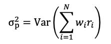
To estimate the risk of a portfolio, MPT uses statistical measures like variance and standard deviation. Variance is calculated to then obtain the standard deviation, which we use to assess the risk of an asset as it indicates how much said asset’s price fluctuates.
On the other hand, correlation and covariance quantify how two assets move compared to each other. Covariance and correlation give an indication of change in value, i.e. Do the assets move in the same way. Correlation is between -1 and 1, a correlation of 1 means that the asset moves in the exact same way and -1 means that they move in opposite ways.
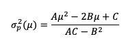
The portfolio variance is calculated as follows for a portfolio of asset A and asset B:

Where:
- R = return
- w = weight of the asset
- Var = variance
- Cov = covariance
The variance of a portfolio is then not equal to the weighted average risk of its components because we factor in the covariance of said components.
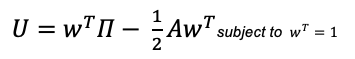
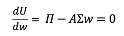
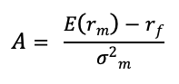
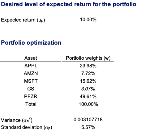
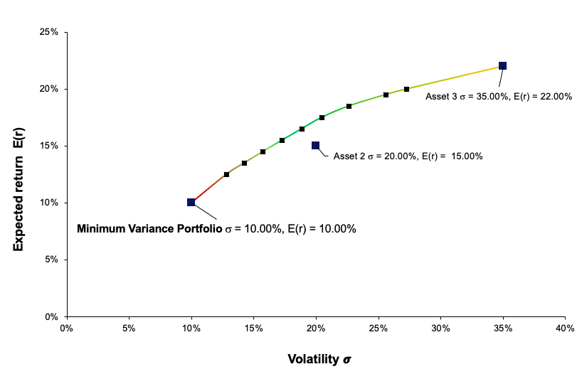
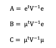
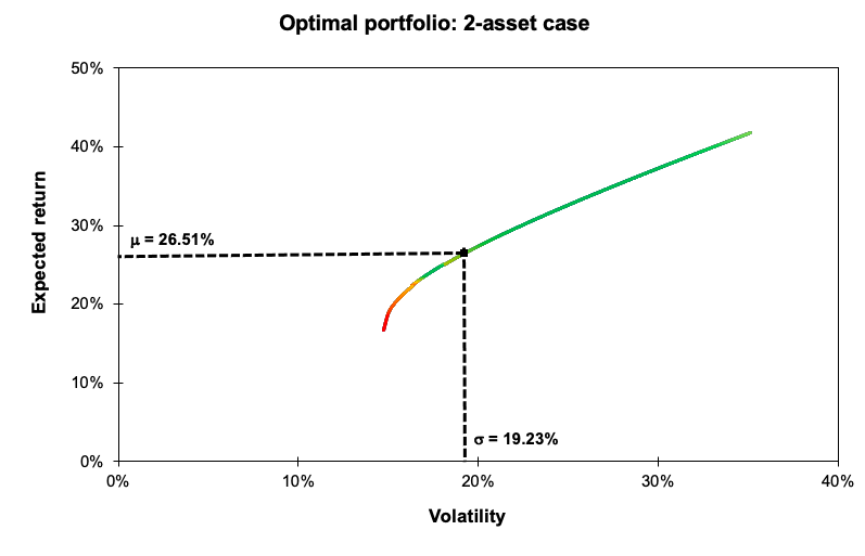
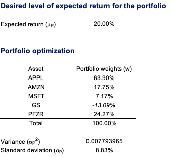
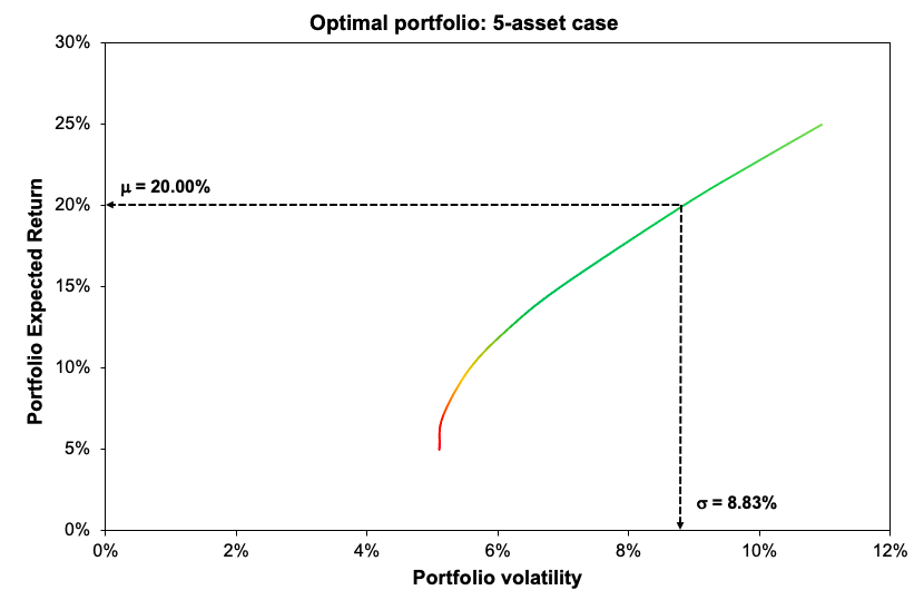
The aim of MPT is to find the optimal portfolio mix that minimizes the portfolio standard deviation for a given level of expected return or that maximizes the portfolio expected return for a given level of standard deviation. This can be graphically represented as the efficient frontier, a line representing the set of optimal portfolios.
This Efficient Frontier represents different allocations of assets in a portfolio. All portfolios on this frontier are called efficient portfolios, meaning that they have the best risk adjusted returns possible with this combination of assets. This means that when choosing the allocation for a portfolio one should pick a portfolio located on the frontier based on their risk tolerance and return objective.
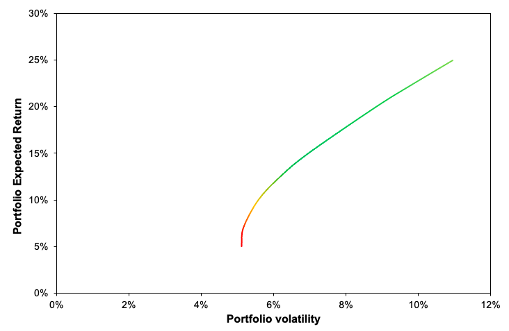
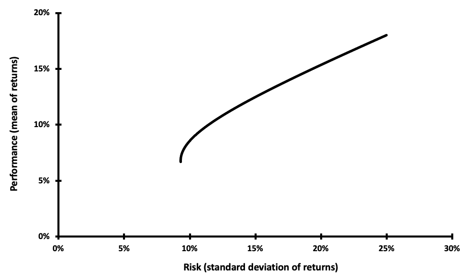
The figure below represents the efficient frontier when investors can invest in risky assets only.
Efficient Portfolio Frontier.
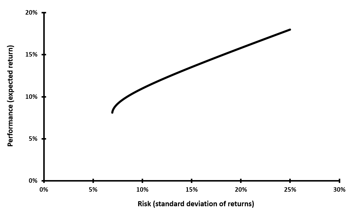
Source: Computation by the Author.
Quantifying performance
To quantify the performance of a portfolio, MPT utilizes Sharpe ratio. The Sharpe ratio measures the excess return of the portfolio (the return over the risk-free rate) for the risk of the portfolio (defined by portfolio standard deviation). The formula is as follows:
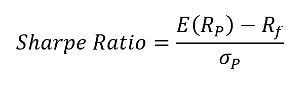
Where:
- E(RP) = expected return of portfolio P
- Rf = risk-free rate
- σP = standard deviation of returns of portfolio P
A higher Sharpe ratio indicates a better risk-adjusted return.
Limitations of MPT
Even though MPT has been around in finance for decades now, it is not universally accepted. The biggest criticism against it is that it employs standard deviation to measure price movement, but the problem is that no difference is made between positive and negative volatility. They are both seen as risky.
However, many investors would be happy with a portfolio that performs 20% or 40% returns every year, but this portfolio could be considered risky by MPT, even if it always performs better than the return needed as there is a lot of variation, however this variation does not matter to you if your return objective is always met. This means that investors care more about downside risks, the risk of performing worse than your return objective.
Emergence of Post-Modern Portfolio Theory (PMPT)
PMPT, introduced in 1991 by software designers Brian M. Rom and Kathleen Ferguson, is a refinement of MPT to overcome its main shortcoming. The key difference lies in the fact that PMPT focuses on downside deviation as a measure of risk, rather than the normal standard deviation that takes every form of deviation into account.
The origins of PMPT can be linked to the work of A. D. Roy with his “Safety First” principle in his 1952 paper, “Safety First and the Holding of Assets”. In his paper, Roy argued that investors are primarily motivated by the desire to avoid disaster rather than to maximize their gains. As he put it, “Decisions taken in practice are less concerned with whether a little more of this or of that will yield the largest net increase in satisfaction than with avoiding known rocks of uncertain position or with deploying forces so that, if there is an ambush round the next corner, total disaster is avoided.” Roy proposed that investors should seek to minimize the probability that their portfolio’s return will fall below a certain minimum acceptable level, or “disaster” level which is now known as MAR for “Minimum Acceptable Return”.
PMPT introduces the concept of the Minimum Acceptable Return (MAR), i.e., the lowest return that the investor wishes to receive. Instead of looking at the overall volatility of a portfolio, PMPT looks only at the returns below the MAR.
Calculating Downside Deviation
To compute downside deviation, we carry out the following:
- Define the Minimum Acceptable Return (MAR).
- Calculate the difference between the portfolio return and the MAR for each period.
- Square the negative differences.
- Sum the squared negative differences.
- Divide by the number of periods.
- Take the square root of the result to obtain the downside deviation.
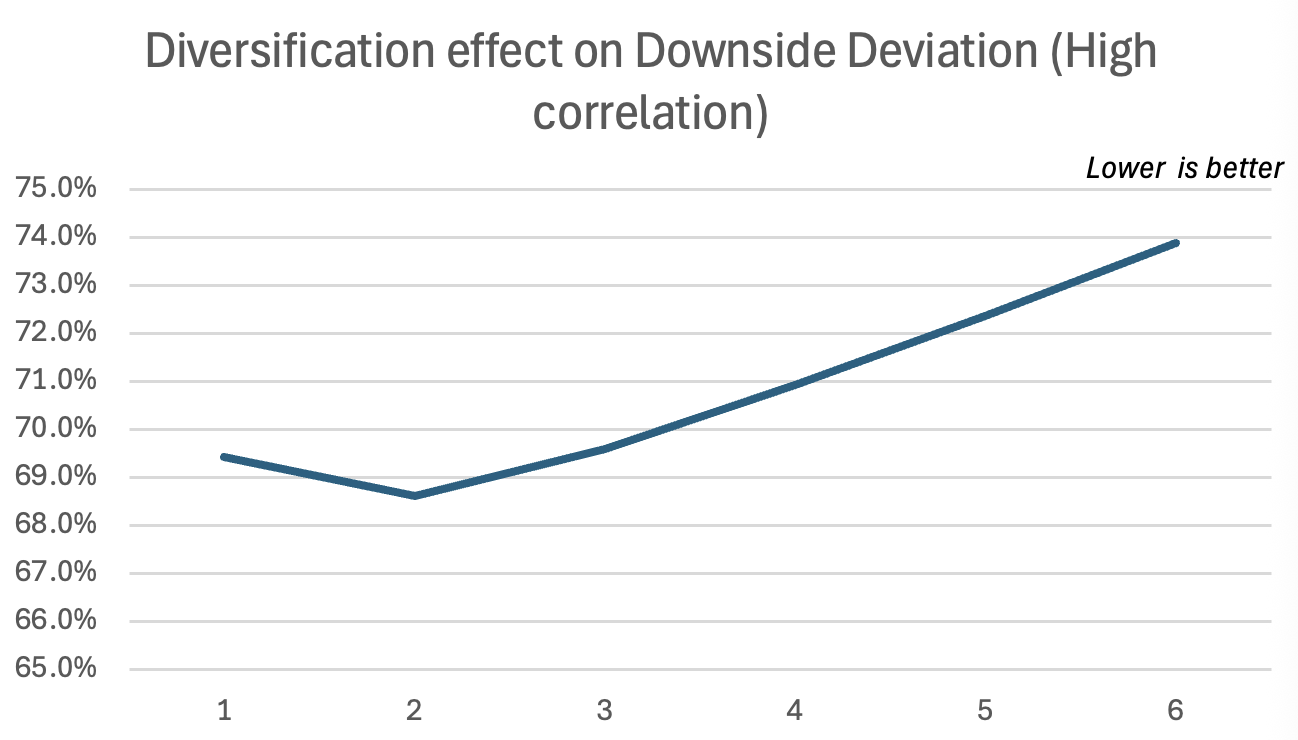
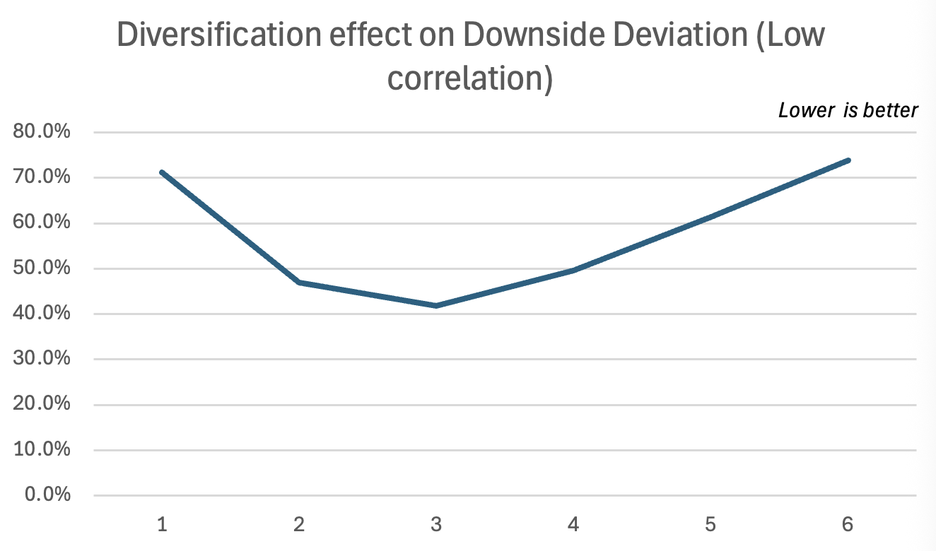
You can download the Excel file below which illustrates the difference between MPT and PMPT with two examples of market conditions (correlation).

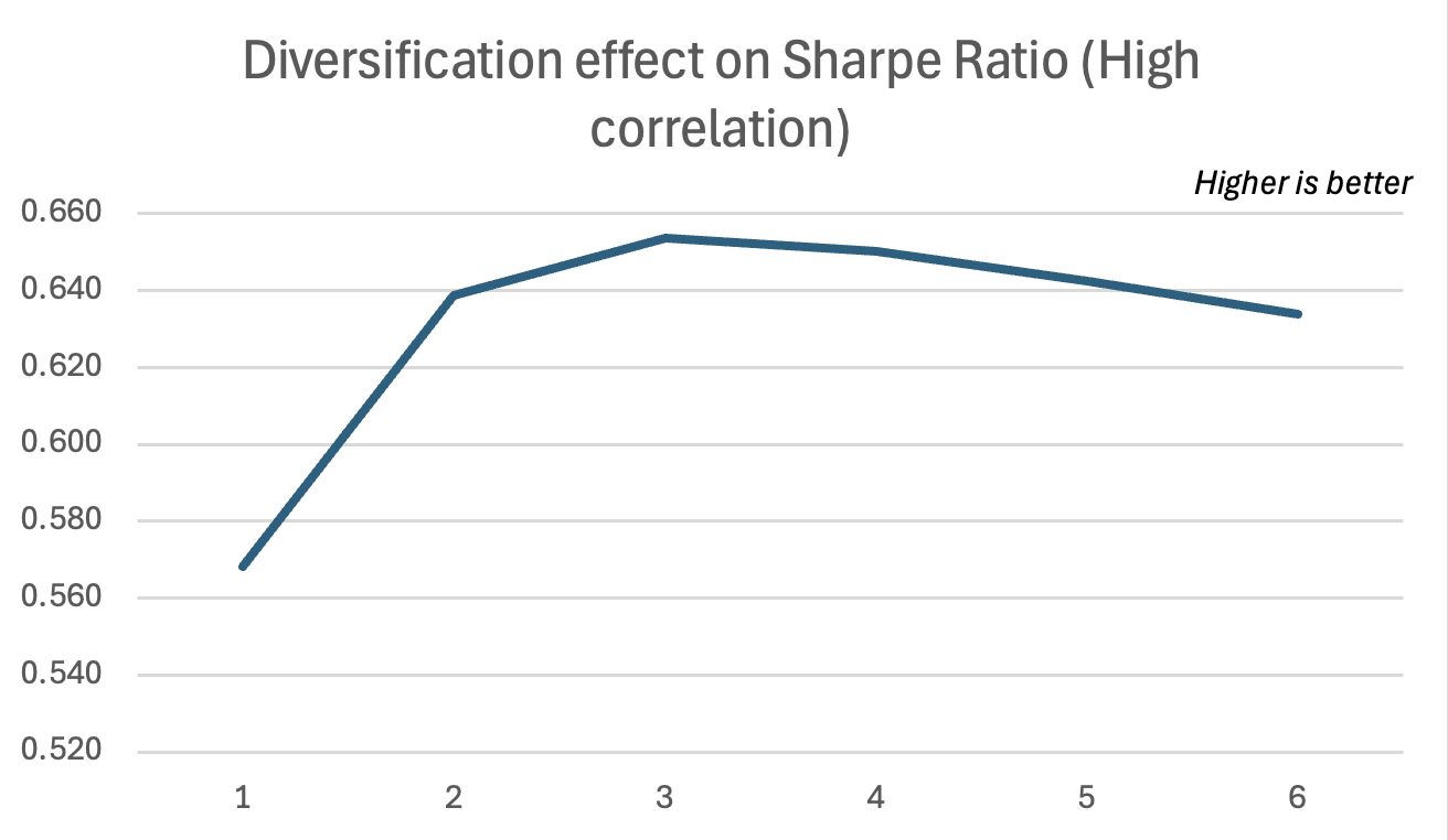
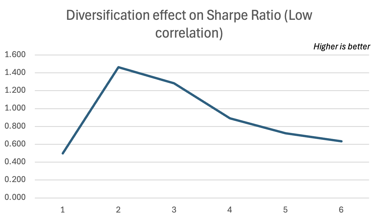
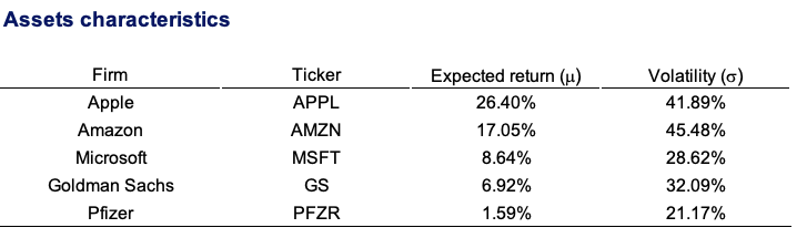
In this file we find 2 combinations of assets: Example 1 and Example 2. The first combination has a positive correlation (0.72) and the second combination a negative one (-0.75) all the while having very similar standard deviation and returns for each asset.
First, using MPT, we demonstrate how high correlation leads to a worsened diversification effect, and a lower increase in portfolio efficiency (Sharpe Ratio) compared to a very similar portfolio with a low correlation.
Afterwards, we use PMPT to show how correlation also impacts the diversification effect through the lens of downside deviation, meaning how much does the portfolio moves below the MAR, keeping in mind that these portfolios have only around a 0.1% difference in average return and originally have almost the same volatility.
Focusing on downside risk is made even more important when you consider that financial returns are rarely normally distributed, as is often assumed in MPT. In their 2004 paper, “Portfolio Diversification Effects of Downside Risk,” Namwon Hyung and Casper G. de Vries show that returns often show signs of what they call “fat tails,” meaning that extreme negative events are more common than a normal distribution would predict.
They find that in this environment; diversification is even more powerful in reducing downside risk. They state: “The VaR-diversification-speed is higher for the class of (finite variance) fat tailed distributions in comparison to the normal distribution”. Meaning that for investors concerned about downside risk, diversification is a more potent tool than they might realize as diversification becomes even more efficient when taking into account the real distribution of returns.
Conclusion
Modern Portfolio Theory has been the main theory used by investors for more than half a century. Its basic premise of diversification and asset allocation is as valid as it ever was. But the usage of Standard Deviation of returns only gives a side of picture, a picture fully captured by PMPT.
Post-Modern Portfolio Theory is more advanced way of managing risk. With its focus on downside deviation, it provides investors with an accurate sense of what they are risking and allows them to build portfolios better aligned with their goals and risk tolerance. MPT was the first iteration, but PMPT has built a more practical framework to effectively diversify a portfolio.
An effective diversification strategy is built on a solid foundation of asset allocation among low-correlation asset classes. By focusing on the quality of diversification rather than only the quantity of holdings, investors can build portfolios that are better aligned with their goals, avoiding the unnecessary costs and diluted returns that come with a diworsified approach.
Why should I be interested in this post?
MPT is a theory widely used in Asset management, the understanding of its principles and limitations is primordial in nowadays financial landscape.
Related posts on the SimTrade blog
▶ Rayan AKKAWI Warren Buffet and his basket of eggs
▶ Raphael TRAEN Understanding Correlation in the Financial Landscape: How It Drives Portfolio Diversification
▶ Rishika YADAV Understanding Risk-Adjusted Return: Sharpe Ratio & Beyond
▶ Youssef LOURAOUI Minimum Volatility Portfolio
▶ All posts about Financial techniques
Useful resources
Ferguson, K. (1994) Post-Modern Portfolio Theory Comes of Age, The Journal of Investing, 1:349-364
Geambasu, C., Sova, R., Jianu, I., and Geambasu, L., (2013) Risk measurement in post-modern portfolio theory: Differences from modern portfolio theory, Economic Computation and Economic Cybernetics Studies and Research, 47:113-132.
Markowitz, H. (1952) Portfolio Selection, The Journal of Finance, 7(1):77–91.
Roy, A.D. (1952) Safety First and the Holding of Assets, Econometrica, 20, 431-449.
Hyung, N., & de Vries, C. G. (2004) Portfolio Diversification Effects of Downside Risk, Working paper.
Sharpe, W.F. (1966) Mutual Fund Performance, Journal of Business, 39(1), 119–138.
Sharpe, W.F. (1994) The Sharpe Ratio, Journal of Portfolio Management, 21(1), 49–58.
About the author
This article was written in October 2025 by Yann TANGUY (ESSEC Business School, Global Bachelor in Business Administration (GBBA), 2023-2027).


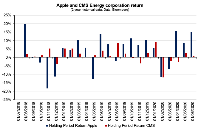
 Computation by the author (data: Bloomberg).